Bayesian astrostatistics: a backward look to the future

Bayesian astrostatistics: a backward look to the future†

arXiv:1208.3036v2 [astro-ph.IM] 29 Aug 2012

Thomas J. Loredo

This perspective chapter briefly surveys: (1) past growth in the use of Bayesian methods in astrophysics; (2) current misconceptions about both frequentist and Bayesian statistical inference that hinder wider adoption of Bayesian methods by astronomers; and (3) multilevel (hierarchical) Bayesian modeling as a major future direction for research in Bayesian astrostatistics, exemplified in part by presentations at the first ISI invited session on astrostatistics, commemorated in this volume. It closes with an intentionally provocative recommendation for astronomical survey data reporting, motivated by the multilevel Bayesian perspective on modeling cosmic populations: that astronomers cease producing catalogs of estimated fluxes and other source properties from surveys. Instead, summaries of likelihood functions (or marginal likelihood functions) for source properties should be reported (not posterior probability density functions), including nontrivial summaries (not simply upper limits) for candidate objects that do not pass traditional detection thresholds.

This volume contains presentations from the first invited session on astrostatistics to be held at an International Statistical Institute (ISI) World Statistics Congress. This session was a major milestone for astrostatistics as an emerging cross-disciplinary research area. It was the first such session organized by the ISI Astrostatistics Committee, whose formation in 2010 marked formal international recognition of the importance and potential of astrostatistics by one of its information science parent disciplines. It was also a significant milestone for Bayesian astrostatistics, as this research area was chosen as a (non-exclusive) focus for the session. As an early (and elder!) proponent of Bayesian methods in astronomy, I have been asked to provide a “perspective piece” on the history and status of Bayesian astrostatistics. I begin by briefly documenting the rapid rise in use of the Bayesian Thomas J. Loredo Center for Radiophysics & Space Research, Cornell University, Ithaca, NY 14853-6801, e-mail: [email protected] † This

paper is a lightly revised version of an invited chapter for Astrostatistical Challenges for the New Astronomy (Joseph M. Hilbe, ed., Springer, New York, 2012), the inaugural volume for the Springer Series in Astrostatistics. The volume commemorates the first invited session on astrostatistics held at an International Statistical Institute (ISI) World Statistics Congress, which took place at the Congress held in Dublin, Ireland in August 2011.

1

2

Thomas J. Loredo

approach by astrostatistics researchers over the past two decades. Next, I describe three misconceptions about both frequentist and Bayesian methods that hinder wider adoption of the Bayesian approach across the broader community of astronomer data analysts. Then I highlight the emerging role of multilevel (hierarchical) Bayesian modeling in astrostatistics as a major future direction for research in Bayesian astrostatistics. I end with a provocative recommendation for survey data reporting, motivated by the multilevel Bayesian perspective on modeling cosmic populations.

1 Looking back Bayesian ideas entered modern astronomical data analysis in the late 1970s, when Steve Gull & Geoff Daniell (1978, 1979) framed astronomical image deconvolution in Bayesian terms.1 Motivated by Harold Jeffreys’ Bayesian Theory of Probability (Jeffreys 1961), and Edwin Jaynes’s introduction of Bayesian and information theory methods into statistical mechanics and experimental physics (Jaynes 1959), they addressed image estimation by writing down Bayes’s theorem for the posterior probability for candidate images, adopting an entropy-based prior distribution for images. They focused on finding a single “best” image estimate based on the posterior: the maximum entropy (MaxEnt) image (maximizing the entropic prior probability subject to a somewhat ad hoc likelihood-based constraint expressing goodness of fit to the data). Such estimates could also be found using frequentist penalized likelihood or regularization approaches. The Bayesian underpinnings of MaxEnt image deconvolution thus seemed more of a curiosity than the mark of a major methodological shift. By about 1990, genuinely Bayesian data analysis—in the sense of reporting Bayesian probabilities for statistical hypotheses, or samples from Bayesian posterior distributions—began appearing in astronomy. The Cambridge MaxEnt group of astronomers and physicists, led by Gull and John Skilling, began developing “quantified MaxEnt” methods to quantify uncertainty in image deconvolution (and other inverse problems), rather than merely reporting a single best-fit image. On the statistics side, Brian Ripley’s group began using Gibbs sampling to sample from posterior distributions for astronomical images based on Markov random field priors (Ripley 1992). My PhD thesis (defended in 1990) introduced parametric Bayesian modeling of Poisson counting and point processes (including processes with truncation or thinning, and measurement error) to high-energy astrophysics (X-ray and gammaray astronomy) and to particle astrophysics (neutrino astronomy). Bayesian methods were just beginning to be used for parametric modeling of ground- and space-based cosmic microwave background (CMB) data (e.g., Readhead & Lawrence 1992). 1 Notably, Peter Sturrock (1973) earlier introduced astronomers to the use of Bayesian probabilities for “bookkeeping” of subjective beliefs about astrophysical hypotheses, but he did not discuss statistical modeling of measurements per se.

Bayesian astrostatistics

3

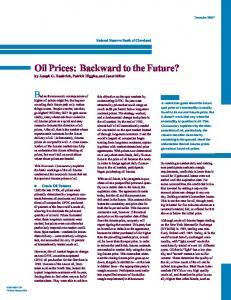
It was in this context that the first session on Bayesian methods to be held at an astronomy conference (to my knowledge) took place, at the first Statistical Challenges in Modern Astronomy conference (SCMA I), hosted by statistician G. Jogesh Babu and astronomer Eric Feigelson at Pennsylvania State University in August 1991. Bayesian methods were not only new, but also controversial in astronomy at that time. Of the 22 papers published in the SCMA I proceedings volume (Feigelson & Babu 1992), only two were devoted to Bayesian methods (Ripley 1992 and Loredo 1992a; see also the unabridged version of the latter, Loredo 1992b).2 Both papers had a strong pedagogical component (and a bit of polemic). Of the 131 SCMA I participants (about 60% astronomers and 40% statisticians), only two were astronomers whose research prominently featured Bayesian methods (Gull and me). Twenty years later, the role of Bayesian methods in astrostatistics research is dramatically different. The 2008 Joint Statistical Meetings included two sessions on astrostatistics predominantly devoted to Bayesian research. At SCMA V, held in June 2011, two sessions were devoted entirely to Bayesian methods in astronomy: “Bayesian analysis across astronomy,” with eight papers and two commentaries, and “Bayesian cosmology,” including three papers with individual commentaries. Overall, 14 of 32 invited SCMA V presentations (not counting commentaries) featured Bayesian methods, and the focus was on calculations and results rather than on pedagogy and polemic. About two months later, the ISI World Congress session on astrostatistics commemorated in this volume was held; as already noted, its focus was Bayesian astrostatistics. On the face of it, these events seem to indicate that Bayesian methods are not only no longer controversial, but are in fact now widely used, even favored for some applications (most notably for parametric modeling in cosmology). But how representative are the conference presentations of broader astrostatistical practice? Fig. 1 shows my amateur attempt at bibliometric measurement of the growing adoption of Bayesian methods in both astronomy and physics, based on queries of publication data in the NASA Astrophysics Data System (ADS). Publication counts indicate significant and rapidly growing use of Bayesian methods in both astronomy and physics.3 Cursory examination of the publications reveals that Bayesian methods are being developed across a wide range of astronomical subdisciplines. It is tempting to conclude from the conference and bibliometric indicators that Bayesian methods are now well-established and well-understood across astronomy. But the conference metrics reflect the role of Bayesian methods in the astrostatistics research community, not in bread-and-butter astronomical data analysis. And as impressive as the trends in the bibliometric metrics may be, the absolute numbers remain small in comparison to all astronomy and physics publications, even limit2 A third paper (Nousek 1992) had some Bayesian content but focused on frequentist evaluation criteria, even for the one Bayesian procedure considered; these three presentations, with discussion, comprised the Bayesian session. 3 Roberto Trotta and Martin Hendry have shown similar plots in various venues, helpfully noting that the recent rate of growth apparent in Fig. 1 is much greater than the rate of growth in the number of all publications; i.e., not just the amount but also the prevalence of Bayesian work is rapidly rising.

4

Thomas J. Loredo

250

1250

Pioneer

Propagation

Popularity

1000

AST Abstracts

200 750

150 500

100 250

50

0 1985

AST+PHY Abstracts

300

1990

1995

Year

2000

2005

0 2010

Fig. 1 Simple bibliometrics measuring the growing use of Bayesian methods in astronomy and physics, based on queries of the NASA ADS database in October 2011. Thick (blue) curves (against the left axis) are from queries of the astronomy database; thin (red) curves (against the right axis) are from joint queries of the astronomy and physics databases. For each case the dashed lower curve indicates the number of papers each year that include “Bayes” or “Bayesian” in the title or abstract. The upper curve is based on the same query, but also counting papers that use characteristically Bayesian terminology in the abstract (e.g., the phrase “posterior distribution” or the acronym “MCMC”); it is meant to capture Bayesian usage in areas where the methods are well-established, with the “Bayesian” appellation no longer deemed necessary or notable.

ing consideration to data-based studies. Although their impact is growing, Bayesian methods are not yet in wide use by astronomers. My interactions with colleagues indicate that significant misconceptions persist about fundamental aspects of both frequentist and Bayesian statistical inference, clouding understanding of how these rival approaches to data analysis differ and relate to one another. I believe these misconceptions play no small role in hindering broader adoption of Bayesian methods in routine data analysis. In the following section I highlight a few misconceptions I frequently encounter. I present them here as a challenge to the Bayesian astrostatistics community; addressing them may accelerate the penetration of sound Bayesian analysis into routine astronomical data analysis.


5

2 Misconceptions For brevity, I will focus on just three important misconceptions I repeatedly encounter about Bayesian and frequentist methods, posed as (incorrect!) “conceptual equations.” They are: • Variability = Uncertainty: This is a misconception about frequentist statistics that leads analysts to think that good frequentist statistics is easier to do than it really is. • Bayesian computation = Hard: This is a misconception about Bayesian methods that leads analysts to think that implementing them is harder than it really is, in particular, that it is harder than implementing a frequentist analysis with comparable capability. • Bayesian = Frequentist + Priors: This is a misconception about the role of prior probabilities in Bayesian methods that distracts analysts from more essential distinguishing features of Bayesian inference. I will elaborate on these faulty equations in turn. Variability = Uncertainty: Frequentist statistics gets its name from its reliance on the long-term frequency conception of probability: frequentist probabilities describe the long-run variability of outcomes in repeated experimentation. Astronomers who work with data learn early in their careers how to quantify the variability of data analysis procedures in quite complicated settings using straightforward Monte Carlo methods that simulate data. How to get from quantification of variability in the outcome of a procedure applied to an ensemble of simulated data, to a meaningful and useful statement about the uncertainty in the conclusions found by applying the procedure to the one actually observed data set, is a subtle problem that has occupied the minds of statisticians for over a century. My impression is that many astronomers fail to recognize the distinction between variability and uncertainty, and thus fail to appreciate the achievements of frequentist statistics and their relevance to data analysis practice in astronomy. The result can be reliance on overly simplistic “home-brew” analyses that at best may be suboptimal, but that sometimes can be downright misleading. A further consequence is a failure to recognize fundamental differences between frequentist and Bayesian approaches to quantification of uncertainty (e.g., that Bayesian probabilities for hypotheses are not statements about variability of results in repeated experiments). To illustrate the issue, consider estimation of the parameters of a model being fit to astronomical data, say, the parameters of a spectral model. It is often straightforward to find best-fit parameters with an optimization algorithm, e.g., minimizing a χ 2 measure of misfit, or maximizing a likelihood function. A harder but arguably more important task is quantifying uncertainty in the parameters. For abundant data, an asymptotic Gaussian approximation may be valid, justifying use of the Hessian matrix returned by many optimization codes to calculate an approximate covariance matrix for defining confidence regions. But when uncertainties are significant and models are nonlinear, we must use more complicated procedures to find accurate confidence regions.

6

Thomas J. Loredo

Bootstrap resampling is a powerful framework statisticians use to develop methods to accomplish this. There is a vast literature on applying the bootstrap idea in various settings; much of it is devoted to the nontrivial problem of devising algorithms that enable useful and accurate uncertainty statements to be derived from simple bootstrap variability calculations. Unfortunately, this literature is little-known in the astronomical community, and too often astronomers misuse bootstrap ideas. The variability-equals-uncertainty misconception appears to be at the root of the problem. As a cartoon example, suppose we have spectral data from a source that we wish to fit with a simple thermal spectral model with two parameters, an amplitude, A (e.g., proportional to the source area and inversely proportional to its distance squared), and a temperature, T (determining the shape of the spectrum as a function of energy or wavelength); we denote the parameters jointly by P = (A, T ). Fig. 2 depicts the two-dimensional (A, T ) parameter space, with the best-fit parameters, ˆ obs ), indicated by the blue four-pointed star. We can use simulated data to find P(D ˆ the variability of the estimator (i.e., of the function P(D) defined by the optimizer) were we to repeatedly observe the source. But how should we simulate data when we do not know the true nature of the signal (and perhaps of noise and instrumental distortions)? And how should the variability of simulation results be used to quantify the uncertainty in inferences based on the one observed dataset? The underlying idea of the bootstrap is to use the observed dataset to define the ensemble of hypothetical data to use in variability calculations, and to find functions of the data (statistics) whose variability can be simply used to quantify uncertainty (e.g., via moments or a histogram). Normally using the observed data to define the ensemble for simulations would be cheating and would invalidate one’s inferences; all frequentist probabilities formally must be “pre-observation” calculations. A major achievement of the bootstrap literature is showing how to use the observed data in a way that gives approximately valid results (hopefully with a rate of conver√ gence better than the O(1/ N) rate achieved by simple Gaussian approximations, for sample size N). One way to proceed is to use the full model we are fitting (both the signal model and the instrument and noise model) to simulate data, with the parameters fixed ˆ obs ) as a surrogate for the true values. Statisticians call this the parametric at P(D bootstrap; it was popularized to astronomers in a well-known paper by Lampton, Margon & Bowyer (1976, hereafter LMB76; statisticians introduced the “parametric bootstrap” terminology later). Alternatively, if some probabilistic aspects of the model are not trusted (e.g., the error distribution is considered unrealistic), an alternative approach is the nonparametric bootstrap, which “recycles” the observed data to generate simulated data (in some simple cases, this may be done by sampling from the observed data with replacement to generate each simulated data set). Whichever approach we adopt, we will generate a set of simulated data, {Di }, to which we can apply our fitting procedure to generate a set of best-fit parameter ˆ i )} that together quantify the variability of our estimator. The black points {P(D dots in Fig. 2 show a scatterplot or “point cloud” of such parameter estimates.


7

A

ˆ obs ) P(D ✦

T Fig. 2 Illustration of the nontrivial relationship between variability of an estimator, and uncertainty of an estimate as quantified by a frequentist confidence region. Shown is a two-dimensional parameter space with a best-fit estimate to the observed data (blue 4-pointed star), best-fit estimates to boostrapped data (black dots) showing variability of the estimator, and a contour bounding a parametric bootstrap confidence region quantifying uncertainty in the estimate.

What does the point cloud tell us about the uncertainty we should associate with the estimate from the observed data (the blue star)? The practice I have seen in too many papers is to interpret the points as samples from a probability distribution in parameter space.4 The cloud itself might be shown, with a contour enclosing a specified fraction of the points offered as a joint confidence region. One-dimensional histograms may be used to find “1σ ” (i.e., 68.3%) confidence regions for particular parameters of interest. Such procedures naively equate variability with uncertainty: the uncertainty of the estimate is identified with the variability of the estimator. Regions created this way are wrong, plainly and simply. They will not cover the true parameters with the claimed probability, and they are skewed in the wrong direction. This is apparent from the figure; the black points are skewed down and to the right of the star indicating the parameter values used to produce the simulated data; the parameters that produced the observed data are thus likely to be up and to the left of the star. In a correct parametric bootstrapping calculation (i.e., with a trusted model), one can use simulated data to calibrate χ 2 or likelihood contours for defining confidence regions. The procedure is not very complicated, and produces regions like the one shown by the contour in Fig. 2, skewed in just the right way; LMB76 described the construction. But frequently investigators are attempting a nonparametric bootstrap, corresponding to a trusted signal model but an untrusted noise model (often this is done without explicit justification, as if nonparametric bootstrapping is the only type 4 I am not providing references to publications exhibiting the problem for diplomatic reasons and for a more pragmatic and frustrating reason: In the field where I have repeatedly encountered the problem—analysis of infrared exoplanet transit data—authors routinely fail to describe their analysis methods with sufficient detail to know what was done, let alone to enable readers to verify or duplicate the analysis. While there are clear signs of statistical impropriety in many of the papers, I only know the details from personal communications with exoplanet transit scientists.

8

Thomas J. Loredo

of bootstrapping). In this case devising a sound bootstrap confidence interval algorithm is not so simple. Indeed, there is a large statistics literature on nonparametric bootstrap confidence intervals, its size speaking to nontrivial challenges in making the bootstrap idea work. In particular, no simple procedure is currently known for finding accurate joint confidence regions for multiple parameters in nonlinear models using the nonparametric bootstrap; yet results purporting to come from such a procedure appear in a number of astronomical publications. Strangely, the most cited reference on bootstrap confidence regions in the astronomical literature is a book on numerical methods, authored by astronomers, with an extremely brief and misleadingly simplistic discussion of the nonparametric bootstrap (and no explicit discussion of parametric bootstrapping). Sadly, this is not the only area where our community appears content disregarding a large body of relevant statistics research (frequentist or otherwise). What explains such disregard of relevant and nontrivial expertise? I am sure there are multiple factors, but I suspect an important one is the misconception that variability may be generically identified with uncertainty. If one believes this, then doing (frequentist) statistics appears to be a simple matter of simulating data to quantify the variability of procedures. For linear models with normally-distributed errors, the identification is practically harmless; it is conceptually flawed but leads to correct results by accident. But more generally, determining how to use variability to quantify uncertainty can be subtle and challenging. Statisticians have worked for a century to establish how to map variability to uncertainty; when we seek frequentist quantifications of uncertainty in nontrivial settings, we need to mine their expertise. Why devote so much space to a misconception about frequentist statistics in a commentary on Bayesian methods? The variability-equals-uncertainty misconception leads data analysts to think that frequentist statistics is easier than it really is, in fact, to think that they already know what they need to know about it. If astronomers realize that sound statistical practice is nontrivial and requires study, they may be more likely to study Bayesian methods, and more likely to come to understand the differences between the frequentist and Bayesian approaches. Also, for the example just described, the way some astronomers misuse the bootstrap is to try to use it to define a probability distribution over parameter space. Frequentist statistics denies such a concept is meaningful, but it is exactly what Bayesian methods aim to provide, e.g., with point clouds produced via Markov chain Monte Carlo (MCMC) posterior sampling algorithms. This brings us to the topic of Bayesian computation. Bayesian computation = Hard: A too-common (and largely unjustified) complaint about Bayesian methods is that their computational implementation is difficult, or more to the point, that Bayesian computation is harder than frequentist computation. Analysts wanting a quick and useable result are thus dissuaded from considering a Bayesian approach. It is certainly true that posterior sampling via MCMC—generating pseudo-random parameter values distributed according to the posterior—is harder to do well than is generating pseudo-random data sets from a best-fit model. (In fact, I would argue that our community may not appreciate how hard it can be to do MCMC well.) But this is an apples-to-oranges comparison between methods making very different types of approximations. Fair comparisons,


9

between Bayesian and frequentist methods with comparable capabilities and approximations, tell a different story. Advocates of Bayesian methods need to tell this story, and give this complaint a proper and public burial. Consider first basic “textbook” problems that are analytically accessible. Examples include estimating the mean of a normal distribution, estimating the coefficients of a linear model (for data with additive Gaussian noise), similar estimation when the noise variance is unknown (leading to Student’s t distribution), estimating the intensity of a Poisson counting process, etc.. In such problems, the Bayesian calculation is typically easier than its frequentist counterpart, sometimes significantly so. Nowhere is this more dramatically demonstrated than in Jeffreys’s classic text, Theory of Probability (1961). In chapter after chapter, Jeffreys solves well-known statistics problems with arguments significantly more straightforward and mathematics significantly more accessible than are used in the corresponding frequentist treatments. The analytical tractability of such foundational problems is an aid to developing sound statistical intuition, so this is not a trivial virtue of the Bayesian approach. (Of course, ease of use is no virtue at all if you reject an approach— Bayesian, frequentist, or otherwise—on philosophical grounds.) Turn now to problems of more realistic complexity, where approximate numerical methods are necessary. The main computational challenge for both frequentist and Bayesian inference is multidimensional integration, over the sample space for frequentist methods, and over parameter space for Bayesian methods. In high dimensions, both approaches tend to rely on Monte Carlo methods for their computational implementation. The most celebrated approach to Bayesian computation is MCMC, which builds a multivariate pseudo-random number generator producing dependent samples from a posterior distribution. Frequentist calculation instead uses Monte Carlo methods to simulate data (i.e., draw samples from the sampling distribution). Building an MCMC posterior sampler, and properly analyzing its output, is certainly more challenging than simulating data from a model, largely because data are usually independently distributed; nonparametric bootstrap resampling of data may sometimes be simpler still. But the comparison is not fair. In typical frequentist Monte Carlo calculations, one simulates data from the best-fit model (or a bootstrap surrogate), not from the true model (or other plausible models). The resulting frequentist quantities are approximate, not just because of Monte Carlo error, but because the integrand (or family of integrands) that would appear in an exact frequentist calculation is being approximated (asymptotically). In some cases, an exact finite-sample frequentist formulation of the problem may not even be known. In contrast, MCMC posterior sampling makes no approximation of integrands; results are approximate only due to Monte Carlo sampling error. No large-sample asymptotic approximations need be invoked. This point deserves amplification. Although the main computational challenge for frequentist statistics is integration over sample space, there are additionally serious theoretical challenges for finite-sample inference in many realistically complex settings. Such challenges do not typically arise for Bayesian inference. These theoretical challenges, and the analytical approximations that are adopted to address them, are ignored in comparisons that pit simple Monte Carlo simulation of data, or

10

Thomas J. Loredo

bootstrapping, against MCMC or other nontrivial Bayesian computation techniques. Arguably, accurate finite-sample parametric inference is often computationally simpler for Bayesian methods, because an accurate frequentist approach is simply impossible, and an approximate calculation can quantify only the rate of convergence of the approximation, not the actual accuracy of the specific calculation being performed. If one is content with asymptotic approximations, the fairer comparison is between asymptotic frequentist and asymptotic Bayesian methods. At the lowest order, asymptotic Bayesian computation using the Laplace approximation is not significantly harder than asymptotic frequentist calculation. It uses the same basic numerical quantities—point estimates and Hessian matrices from an optimizer—but in different ways. It provides users with nontrivial new capabilities, such as the ability to marginalize over nuisance parameters, or to compare models using Bayes factors that include an “Ockham’s razor” penalty not present in frequentist significance tests, and that enable straightforward comparison of rival models that need not be nested (with one being a special case √ of the other). And the results are sometimes accurate to one order higher (in 1/ N) than corresponding frequentist results (making them potentially competitive with some bootstrap methods seeking similar asymptotic approximation rates). Some elaboration of these issues is in Loredo (1999), including references to literature on Bayesian computation up to that time. A more recent discussion of this misconception about Bayesian methods (and other misconceptions) is in an insightful essay by the Bayesian economist Christopher Sims, winner of the 2011 Nobel Prize in economics (Sims 2010). Bayesian = Frequentist + Priors: I recently helped organize and present two days of tutorial lectures on Bayesian computation, as a prelude to the SCMA V conference mentioned above. As I was photocopying lecture notes for the tutorials, a colleague walked into the copy room and had a look at the table of contents for the tutorials. “Why aren’t all of the talks about priors?” he asked. In response to my puzzled look, he continued, “Isn’t that what Bayesian statistics is about, accounting for prior probabilities?” Bayesian statistics gets its name from Bayes’s theorem, establishing that the posterior probability for a hypothesis is proportional to the product of its prior probability, and the probability for the data given the hypothesis (i.e., the sampling distribution for the data). The latter factor is the likelihood function when considered as a function of the hypotheses being considered (with the data fixed to their observed values). Frequentist methods that directly use the likelihood function, and their least-squares cousins (e.g., χ 2 minimization), are intuitively appealing to astronomers and widely used. On the face of it, Bayes’s theorem appears merely to add modulation by a prior to likelihood methods. By name, Bayesian statistics is evidently about using Bayes’s theorem, so it would seem it must be about how frequentist results should be altered to account for prior probabilities. It would be hard to overstate how wrong this conception of Bayesian statistics is. The name is unfortunate; Bayesian statistics uses all of probability theory, not just Bayes’s theorem, and not even primarily Bayes’s theorem. What most funda-


11

mentally distinguishes Bayesian calculations from frequentist calculations is not modulation by priors, but the key role of probability distributions over parameter (hypothesis) space in the former, and the complete absence of such distributions in the latter. Via Bayes’s theorem, a prior enables one to use the likelihood function—describing a family of measures over the sample space—to build the posterior distribution—a measure over the parameter (hypothesis) space (where by “measure” I mean an additive function over sets in the specified space). This construction is just one step in inference. Once it happens, the rest of probability theory kicks in, enabling one to assess scientific arguments directly by calculating probabilities quantifying the strengths of those arguments, rather than indirectly, by having to devise a way that variability of a cleverly chosen statistic across hypothetical data might quantify uncertainty across possible choices of parameters or models for the actually observed data. Perhaps the most important theorem for doing Bayesian calculations is the law of total probability (LTP) that relates marginal probabilities to sums of joint and conditional probabilities. To display its role, suppose we are analyzing some observed data, Dobs , using a parametric model with parameters θ . Let M denote all the modeling assumptions—definitions of the sample and parameter spaces, description of the connection between the model and the data, and summaries of any relevant prior information (parameter constraints or results of other measurements). Now consider some of the common uses of LTP in Bayesian analysis: • Calculating the probability in a credible region, R, for θ : p(θ ∈ R|Dobs ) =

Z

R

d θ p(θ ∈ R|θ ) p(θ |Dobs )

|| M,

(1)

where p(θ |Dobs , M) is the posterior probability density for θ . Here I have introduced a convenient shorthand due to John Skilling: “||M” indicates that M is conditioning information common to all displayed probabilities. • Calculating a marginal posterior distribution when a vector parameter θ = (ψ , η ) has both an interesting subset of parameters, ψ , and uninteresting “nuisance” parameters, η . The uncertainty in ψ (with the η uncertainty fully propagated) is quantified by the marginal density, p(ψ |Dobs ) =

Z

d η p(ψ , η |Dobs )

|| M.

(2)

• Predicting future data, D′ , with the posterior predictive distribution, p(D′ |Dobs ) =

Z

d θ p(D′ |θ ) p(θ |Dobs )

|| M,

(3)

with the integration accounting for parameter uncertainty in the prediction. • Comparing rival parametric models Mi (each with parameters θi ) via posterior odds or Bayes factors, which requires computation of the marginal likelihood for each model given by

12

Thomas J. Loredo

p(Dobs |Mi ) =

Z

d θi p(θi |Mi ) p(Dobs |θi , Mi )

|| M1 ∨ M2 . . . .

(4)

In words, this says that the likelihood for a model is the average of the likelihood function for that model’s parameters. Arguably, if this approach to inference is to be named for a theorem, “total probability inference” would be a more appropriate appellation than “Bayesian statistics.” It is probably too late to change the name. But it is not too late to change the emphasis. In axiomatic developments of Bayesian inference, priors play no fundamental role; rather, they emerge as a required ingredient when one seeks a consistent or coherent calculus for the strengths of arguments that reason from data to hypotheses. Sometimes priors are eminently useful, as when one wants to account for a positivity constraint on a physical parameter, or to combine information from different experiments or observations. Other times they are frankly a nuisance, but alas still a necessity. A physical analogy I find helpful for elucidating the role of priors in Bayesian inference appeals to the distinction between intensive and extensive quantities in thermodynamics. Temperature is an intensive property; in a volume of space it is meaningful to talk about the temperature T (x) at a point x, but not about the “total temperature” of the volume; temperature does not add or integrate across space. In contrast, heat is an extensive property, an additive property of volumes; in mathematical parlance, it may be described by a measure (a mapping from regions, rather than points, to a real number). Temperature and heat are related; the heat in a volR ume V is given by Q = V dx [ρ (x)c(x)]T (x), where ρ (x) is the density and c(x) is the specific heat capacity. The product ρ c is extensive, and serves to convert the intensive temperature to its extensive relative, heat. In Bayesian inference, the prior plays an analogous role, not just “modulating” likelihood, but converting intensive likelihood to extensive probability. In thermodynamics, a region with a high temperature may have a small amount of heat if its volume is small, or if, despite having a large volume, the value of ρ c is small. In Bayesian statistics, a region of parameter space with high likelihood may have a small probability if its volume is small, or if the prior assigns low probability to the region. This accounting for volume in parameter space is a key feature of Bayesian methods. What makes it possible is having a measure over parameter space. Priors are important, not so much as modulators of likelihoods, but as converters from intensities (likelihoods) to measures (probabilities). With poetic license, one might say that frequentist statistics focuses on the “hottest” (highest likelihood) hypotheses, while Bayesian inference focuses on hypotheses with the most “heat” (probability). Incommensurability: The growth in the use of Bayesian methods in recent decades has sometimes been described as a “revolution,” presumably alluding to Thomas Kuhn’s concept of scientific revolutions (Kuhn 1970). Although adoption of Bayesian methods in many disciplines has been growing steadily and sometimes dramatically, Bayesian methods have yet to completely or even substantially replace frequentist methods in any broad discipline I am aware of (although this has happened in some


13

subdisciplines). I doubt the pace and extent of change qualifies for a Kuhnian revolution. Also, the Bayesian and frequentist approaches are not rival scientific theories, but rather rival paradigms for a part of the scientific method itself (how to build and assess arguments from data to scientific hypotheses). Nevertheless, the competition between Bayesian and frequentist approaches to inference does bear one hallmark of a Kuhnian revolution: incommensurability. I believe Bayesian-frequentist incommensurability is not well-appreciated, and that it underlies multiple misconceptions about the approaches. Kuhn insisted that there could be no neutral or objective measure allowing comparison of competing paradigms in a budding scientific revolution. He based this claim on several features he found common to scientific revolutions, including the following: (1) Competing paradigms often adopt different meanings for the same term or statement, making it very difficult to effectively communicate across paradigms (a standard illustration is the term “mass,” which takes on different meanings in Newtonian and relativistic physics). (2) Competing paradigms adopt different standards of evaluation; each paradigm typically “works” when judged by its own standards, but the standards themselves are of limited use in comparing across paradigms. These aspects of Kuhnian incommensurability are evident in the frequentist and Bayesian approaches to statistical inference. (1) The term “probability” takes different meanings in frequentist and Bayesian approaches to uncertainty quantification, inviting misunderstanding when comparing frequentist and Bayesian answers to a particular inference problem. (2) Long-run performance is the gold standard for frequentist statistics; frequentist methods aim for specified performance across repeated experiments by construction, but make no probabilistic claims about the result of application of a procedure to a particular observed dataset. Bayesian methods adopt more abstract standards, such as coherence or internal consistency, that apply to inference for the case-at-hand, with no fundamental role for frequencybased long-run performance. A frequentist method with good long-run performance can violate Bayesian coherence or consistency requirements so strongly as to be obviously unacceptable for inference in particular cases.5 On the other hand, Bayesian algorithms do not have guaranteed frequentist performance; if it is of interest, it must be separately evaluated, and priors may need adjustment to improve frequentist performance.6 Kuhn considered rival paradigms to be so “incommensurable” that “proponents of competing paradigms practice their trades in different worlds.” He argued that 5 Efron (2003) describes some such cases by saying the frequentist result can be accurate but not correct. Put another way, the performance claim is valid, but the long-run performance can be irrelevant to the case-at-hand, e.g., due to the existance of so-called recognizable subsets in the sample space (see Loredo (1992) and Efron (2003) for elaboration of this notion). This is a further example of how nontrivial the relationship between variability and uncertainty can be. 6 There are theorems linking single-case Bayesian probabilities and long-run performance in some general settings, e.g., establishing that, for fixed-dimension parametric inference, Bayesian credible regions with probability P have frequentist coverage close to P (the rate of convergence is √ O(1/ N) for flat priors, and faster for so-called reference priors). But the theorems do not apply in some interesting classes of problems, e.g., nonparametric problems.

14

Thomas J. Loredo

incommensurability is often so stark that for an individual scientist to adopt a new paradigm requires a psychological shift that could be termed a “conversion experience.” Following Kuhn, philosophers of science have debated how extreme incommensurability really is between rival paradigms, but the concept is widely considered important for understanding significant changes in science. In this context, it is notable that statisticians, and scientists more generally, often adopt a particular almost-religious terminology in frequentist vs. Bayesian discussions: rather than a method being described as frequentist or Bayesian, the investigator is so described. This seems to me to be an unfortunate tradition that should be abandoned. Nevertheless, it does highlight the fundamental incommensurability between these rival paradigms for uncertainty quantification. Advocates of one approach or the other (or of a nuanced combination) need to more explicitly note and discuss this incommensurability, especially with nonexperts seeking to choose between approaches. The fact that both paradigms remain in broad use suggests that ideas from both approaches may be relevant to inference; perhaps they are each suited to addressing different types of scientific questions. For example, my discussion of misconceptions has been largely from the perspective of parametric modeling (parameter estimation and model comparison). Nonparametric inference raises more subtle issues regarding both computation and the role of long-term performance in Bayesian inference; see Bayarri & Berger (2004) and Sims (2010) for insightful discussions of some of these issues. Also, Bayesian model checking (assessing the adequacy of a parametric model without an explicitly specified class of alternatives) typically invokes criteria based on predictive frequencies (Bayarri & Berger 2004; Gelman et al. 2004; Little 2006). A virtue of the Bayesian approach is that one may predict or estimate frequencies when they are deemed relevant; explicitly distinguishing probability (as degree of strength of an argument) from frequency (in finite or hypothetical infinite samples) enables this. This suggests some kind of unification of approaches may be easier to achieve from the Bayesian direction. This is a worthwhile task for research; see Loredo (2012a) for a brief overview of some recent work on the Bayesian/frequentist interface. No one would claim that the Bayesian approach is a data analysis panacea, providing the best way to address all data analysis questions. But among astronomers outside of the community of astrostatistics researchers, Bayesian methods are significantly underutilized. Clearing up misconceptions should go a long way toward helping astronomers appreciate what both frequentist and Bayesian methods have to offer for both routine and research-level data analysis tasks.

3 Looking forward Having looked at the past growth of interest in Bayesian methods and present misconceptions, I will now turn to the future. As inspiration, I cite Mike West’s commentary on my SCMA I paper (West 1992). In his closing remarks he pointed to an especially promising direction for future Bayesian work in astrostatistics:


15

On possible future directions, it is clear that Bayesian developments during recent years have much to offer—I would identify prior modeling developments in hierarchical models as particularly noteworthy. Applications of such models have grown tremendously in biomedical and social sciences, but this has yet to be paralleled in the physical sciences. Investigations involving repeat experimentation on similar, related systems provide the archetype logical structure for hierarchical modeling. . . There are clear opportunities for exploitation of these (and other) developments by astronomical investigators. . . .

However clear the opportunities may have appeared to West, for over a decade following SCMA I, few astronomers pursued hierarchical Bayesian modeling. A particularly promising application area is modeling of populations of astronomical sources, where hierarchical models can naturally account for measurement error, selection effects, and “scatter” of properties across a population. I discussed this at some length at SCMA IV in 2006 (Loredo 2007), but even as of that time there was relatively little work in astronomy using hierarchical Bayesian methods, and for the most part only the simplest such models were used. The last few years mark a change point in this respect, and evidence of the change is apparent in the contributions to the summer 2011 Bayesian sessions at both SCMA V and the ISI World Congress. Several presentations in both forums described recent and ongoing research developing sophisticated hierarchical models for complex astronomical data. Other papers raised issues that may be addressed with hierarchical models. Together, these papers point to hierarchical Bayesian modeling as an important emerging research direction for astrostatistics. To illustrate the notion of a hierarchical model—also known as a multilevel model (MLM)—we start with a simple parametric density estimation problem, and then promote it to a MLM by adding measurement error. Suppose we would like to estimate parameters θ defining a probability density function f (x; θ ) for an observable x. A concrete example might be estimation of a galaxy luminosity function, where x would be two-dimensional, x = (L, z) for luminosity L and redshift z, and f (x; θ ) would be the normalized luminosity function (i.e., a probability density rather than a galaxy number density). Consider first the case where we have a set of precise measurements of the observables, {xi } (and no selection effects). Panel (a) in Fig. 3 depicts this simple setting. The likelihood function for θ is L (θ ) ≡ p({xi }|θ , M) = ∏i f (xi ; θ ). Bayesian estimation of θ requires a prior density, π (θ ), leading to a posterior density p(θ |{xi }, M) ∝ π (θ )L (θ ). An alternative way to write Bayes’s theorem expresses the posterior in terms of the joint distribution for parameters and data: p(θ |{xi }, M) =

p(θ , {xi }|M) . p({xi }|M)

(5)

This “probability for everything” version of Bayes’s theorem changes the process of modeling from separate specification of a prior and likelihood, to specification of the joint distribution for everything; this proves helpful for building models with complex dependencies. Panel (c) depicts the dependencies in the joint distribution with a graph—a collection of nodes connected by edges—where each node represents a probability distribution for the indicated variable, and the directed edges indicate

16

Thomas J. Loredo

Fig. 3 Illustration of multilevel model approach to handling measurement error. (a) and (b) (top row): Measurements of a two-dimensional observable and its probability distribution (contours); in (a) the measurements are precise (points); in (b) they are noisy (filled circles depict uncertainties). (c) and (d): Graphical models corresponding to Bayesian estimation of the density in (a) and (b), respectively.

dependences between variables. Shaded nodes indicate variables whose values are known (here, the data); we may manipulate the joint to condition on these quantities. The graph structure visually displays how the joint distribution may be factored as a sequence of independent and conditional distributions: the θ node represents the prior, and the xi nodes represent f (xi ; θ ) = p(xi |θ , M) factors, dependent on θ but independent of other xi values when θ is given (i.e., conditionally independent). The joint distribution is thus p(θ , {xi }|M) = π (θ ) ∏i f (xi ; θ ). In a sense, the most important edges in the graph are the missing edges; they indicate independence that makes factors simpler than they might otherwise be. Now suppose that, instead of precise xi measurements, for each observation we get noisy data, Di , producing a measurement likelihood function ℓi (xi ) ≡ p(Di |xi , M) describing the uncertainties in xi (we might summarize it with the mean and standard deviation of a Gaussian). Panel (b) depicts the situation; instead of points in x space, we now have likelihood functions (depicted as “1σ ” error circles). Panel (d) shows a graph describing this measurement error problem, which adds a {Di } level to the previous graph; we now have a multilevel model.7 The xi nodes are now unshaded; they are no longer known, and have become latent parameters. From the graph we can read off the form of the joint distribution: 7

The convention is to reserve the term for models with three or more levels of nodes, i.e., two or more levels of edges, or two or more levels of nodes for uncertain variables (i.e., unshaded nodes). The model depicted in panel (d) would be called a two-level model.


17

p(θ , {xi }, {Di }|M) = π (θ ) ∏ f (xi ; θ )ℓi (xi ).

(6)

i

From this joint distribution we can make inferences about any quantity of interest. To estimate θ , we use the joint to calculate p(θ , {xi }|{Di }, M) (i.e., we condition on the known data using Bayes’s theorem), and then we marginalize over all of the latent xi variables. We can estimate all the xi values jointly by instead marginalizing over θ . Note that this produces a joint marginal distribution for {xi } that is not a product of independent factors; although the xi values are conditionally independent given θ , they are marginally dependent. If we do not know θ , each xi tells us something about all the others through what it tells us about θ . Statisticians use the phrase “borrowing strength” to describe this effect, from John Tukey’s evocative description of “mustering and borrowing strength” from related data in multiple stages of data analysis (see Loredo and Hendry 2010 for a tutorial discussion of this effect and the related concept of shrinkage estimators). Note the prominent role of LTP in inference with MLMs, where inference at one level requires marginalization over unknowns at other levels. The few Bayesian MLMs used by astronomers through the 1990s and early 2000s did not go much beyond this simplest hierarchical structure. For example, unbeknownst to West, at the time of his writing my thesis work had already developed a MLM for analyzing the arrival times and energies of neutrinos detected from SN 1987A; the multilevel structure was needed to handle measurement error in the energies (an expanded version of this work appears in Loredo & Lamb 2002). Panel (a) of Fig. 4 shows a graph describing the model. The rectangles are “plates” indicating substructures that are repeated; the integer variable in the corner indicates the number of repeats. There are two plates because neutrino detectors have a limited (and energy-dependent) detection efficiency. The plate with a known repeat count, N, corresponds to the N detected neutrinos with times t and energies ε ; the plate with an unknown repeat count, N, corresponds to undetected neutrinos, which must be considered in order to constrain the total signal rate; D denotes the nondetection data, i.e., reports of zero events in time intervals between detections. Other problems tackled by astronomers with two-level MLMs include: modeling of number-size distributions (“logN–log S” or “number counts”) of gamma-ray bursts and trans-Neptunian objects (e.g., Loredo & Wasserman 1998; Petit et al. 2008); performing linear regression with measurement error along both axes, e.g., for correlating quasar hardness and luminosity (Kelly 2007; see his contribution in Feigelson & Babu 2012 for an introduction to MLMs for measurement error) and for correlating galaxy cluster richness and mass (Andreon & Hurn 2010); accounting for Eddington and Malmquist biases in cosmology (Loredo & Hendry 2010); statistical assessment of directional coincidences with gamma-ray bursts (Luo, Loredo & Wasserman 1996; Graziani & Lamb 1996) and cross-matching catalogs produced by large star and galaxy surveys (Budav´ari & Szalay 2008; see Loredo 2012b for discussion of the underlying MLM); and handling multivariate measurement error when estimating stellar velocity distributions from proper motion survey data (Bovy, Hogg, & Roweis 2011).

18

Thomas J. Loredo

Fig. 4 Graphs describing multilevel models used in astronomy, as described in the text.

Beginning around 2000, interdisciplinary teams of astronomers and information scientists began developing significantly more sophisticated MLMs for astronomical data. The most advanced such work has come from a collaboration of astronomers and statisticians associated with the Harvard-Smithsonian Center for Astrophysics (CfA). Much of their work has been motivated by analysis of data from the Chandra X-ray observatory satellite, whose science operations are managed by CfA. van Dyk et al. (2001) developed a many-level MLM for fitting Chandra X-ray spectral data; a host of latent parameters enable accurate accounting for uncertain backgrounds and instrumental effects such as pulse pile-up. Esch et al. (2004) developed a Bayesian image reconstruction algorithm for Chandra imaging data that uses a multiscale hierarchical prior to build spatially-adaptive smoothing into image estimation and uncertainty quantification. van Dyk et al. (2009) showed how to analyze stellar cluster color-magnitude diagrams (CMDs) using finite mixture models (FMMs) to account for contamination of the data from stars not lying in the targeted cluster. In FMMs, categorical class membership variables appear as latent parameters; the mixture model effectively averages over many possible graphs (corresponding to different partitions of the data into classes; such averaging over partitions also appears in the Bayesian cross-matching framework of Luo, Loredo & Wasserman 1996). FMMs have long been used to handle outliers and contamination in Bayesian regression and density estimation. This work showed how to implement it with computationally expensive models and informative class membership priors. In the area of time series, the astronomer-engineer collaboration of


19

Dobigeon, Tourneret, & Scargle (2007) developed a three-level MLM to tackle joint segmentation of astronomical arrival time series (a multivariate extension of Scargle’s well-known Bayesian Blocks algorithm). Cosmology is a natural arena for multilevel modeling, because of the indirect link between theory and observables. For example, in modeling both the cosmic microwave background (CMB) and the large scale structure (LSS) of the galaxy distribution, theory does not predict a specific temperature map or set of galaxy locations (these depend on unknowable initial conditions), but instead predicts statistical quantities, such as angular or spatial power spectra. Modeling observables given theoretical parameters typically requires introducing these quantities as latent parameters. In Loredo (1995) I described a highly simplified hierarchical treatment of CMB data, with noisy CMB temperature difference time series data at the lowest level, l = 2 spherical harmonic coefficients in the middle, and a single physical parameter of interest, the cosmological quadrupole moment Q, at the top. While a useful illustration of the MLM approach, I noted there were enormous computational challenges facing a more realistic implementation. It took a decade for such an implementation to be developed, in the pioneering work of Wandelt et al. (2004). And only recently have explicit hierarchical models been implemented for LSS modeling (e.g., Kitaura & Enßlin 2008). This brings us to the present. Contributions in this volume and in the SCMA V proceedings (Feigelson & Babu 2012) document burgeoning interest in Bayesian MLMs among astrostatisticians. I discuss the role of MLMs in the SCMA V contributions elsewhere (Loredo 2012c). Four of the contributions in the present volume rely on MLMs. Two address complex problems and help mark an era of new complexity and sophistication in astrophysical MLMs. Two highlight the potential of basic MLMs for addressing common astronomical data analysis problems that defy accurate analysis with conventional methods taught to astronomers. I will highlight the MLM aspects of these contributions in turn. Some of the most impressive new Bayesian multilevel modeling in astronomy addresses the analysis of measurements of multicolor light curves (brightness vs. time in various wavebands) from Type Ia supernovae (SNe Ia). In the late 1990s, astronomers discovered that these enormous stellar thermonuclear exoplosions are “standardizable candles;” the shapes of their light curves are strongly correlated with their luminosities (the intrinsic amplitudes of the light curves). This enables use of SNe Ia to measure cosmic distances (via a generalized inverse-square law) and to trace the history of cosmic expansion. The 2011 Nobel Prize in physics went to three astronomers who used this capability to show that the expansion rate of the universe is growing with time (“cosmic acceleration”), indicating the presence of “dark energy” that somehow prevents the deceleration one would expect from gravitational attraction. A high-water mark in astronomical Bayesian multilevel modeling was set by Mandel et al. (2011), who address the problem of estimating supernova luminosities from light curve data. Their model has three levels, complex connections between latent variables (some of them random functions—light curves—rather than scalars), and jointly describes three different types of data (light curves, spectra, and

20

Thomas J. Loredo

host galaxy spectroscopic redshifts). Panel (b) of Fig. 4 shows the graph for their MLM (the reader will have to consult Mandel et al. (2011), or Mandel’s more tutorial overview in Feigelson & Babu (2012), for a description of the variables and the model). In this volume, March et al. tackle a subsequent SNe Ia problem: how to use the output of light curve models to estimate cosmological parameters, including the density of dark energy, and an “equation of state” parameter aiming to capture how the dark energy density may be evolving. Their framework can fuse information from SN Ia with information from other sources, such as the power spectrum of CMB fluctuations, and characterization of the baryon acoustic oscillation (BAO) seen in the large scale spatial distribution of galaxies. Panel (c) of Fig. 4 shows the graph for their model, also impressive for its complexity (see their contribution in this volume for an explanation of this graph). I display the graphs (without much explanation) to show how much emerging MLM research in astronomy is leapfrogging the simple models of the recent past, exemplified by Panel (a) in the figure. Section 3.4 of Andreon’s tutorial in this volume discusses essentially the same model. Equally impressive is Wandelt’s contribution, describing a hierarchical Bayes approach (albeit without explicit MLM language) for reconstructing the galaxy density field from noisy photometric redshift data measuring the line-of-sight velocities of galaxies (which includes a component from cosmic expansion and a “peculiar velocity” component from gravitational attraction of nearby galaxies and dark matter). His team’s framework (described in detail by Jasche & Wandelt 2011) includes nonparametric estimation of the density field at an upper level, which adaptively influences estimation of galaxy distances and peculiar velocities at a lower level, borrowing strength in the manner described above. The nonparametric upper level, and the size of the calculation, make this work groundbreaking. The contributions by Andreon and by Kunz et al. describe simpler MLMs, but with potentially broad applicability. Andreon’s galaxy cluster mass prediction example describes regression with measurement error (fitting lines and curves using data with errors in both the abscissa and ordinate) using a basic MLM. Such problems are common in astronomy. Kelly (2007; see also Kelly’s more introductory treatment in Feigelson & Babu 2012) provided a more formal account of the Bayesian treatment of such problems, drawing on the statistics literature on measurement error problems (e.g., Carroll et al. 2006). The complementary emphasis of Andreon’s account is on how straightforward—indeed, almost automatic—implementation can be using modern software packages such as BUGS and JAGS,8 a point also discussed (a bit more critically) by Carroll et al. (2006). The contribution by Kunz et al. further develops the Bayesian estimation applied to multiple species (BEAMS) framework first described by Kunz et al. (2007). BEAMS aims to improve parameter estimation in nonlinear regression when the data may come from different types of sources (“species” or classes), with different error or population distributions, but with uncertainty in the type of each datum. The classification labels for the data become discrete latent parameters in a MLM; marginalizing over them (and possibly esti8

http://www.mrc-bsu.cam.ac.uk/bugs/


21

mating parameters in the various error distributions) can greatly improve inferences. They apply the approach to estimating cosmological parameters using SNe Ia data, and show that accounting for uncertainty in supernova classification has the potential to significantly improve the precision and accuracy of estimates. In the context of this volume, one cannot help but wonder what would come of integrating something like BEAMS into the MLM framework of March et al.. In Section 2 I noted how the “variability = uncertainty” misconception leads many astronomers to ignore relevant frequentist statistics literature; it gives the analyst the impression that the ability to quantify variability is all that is needed to devise a sound frequentist procedure. There is a similar danger for Bayesian inference. Once one has specified a model for the data (embodied in the likelihood function), Bayesian inference appears to be automatic in principle; one just follows the rules of probability theory to calculate probabilities for hypotheses of interest (after assigning priors). But despite the apparent simplicity of the sum and product rules, probability theory can exhibit a sophisticated subtlety, with apparently innocuous assumptions and calculations sometimes producing surprising results. The huge literature on Bayesian methods is more than mere crank turning; it amasses significant experience with this sophisticated machinery that astronomers should mine to guide development of new Bayesian methods, or to refine existing ones. For this non-statistician reader, it is the simpler of the contributions in this volume— those by Andreon and by Kunz et al.—that point to opportunities for “borrowing and mustering of strength” from earlier work by statisticians. Andreon’s “de-TeXing” approach to Bayesian modeling (i.e., transcribing model equations to BUGS or JAGS code, and assigning simple default priors) is both appealing and relatively safe for simple models, such as standard regression (parametric curve fitting with errors only in the ordinate) or density estimation from precise point measurements in low dimensions. But the implications of modeling assumptions become increasingly subtle as model complexity grows, particularly when one starts increasing the number of levels or the dimensions of model components (or both). Nontrivial computational challenges may also ensue. This makes me wary of emphasizing an automated style of Bayesian modeling. Let us focus here on some MLM subtlety that can complicate matters. Information gain from the data tends to weaken as one considers parameters at increasingly high levels in a multilevel model (Goel & DeGroot 1981). On the one hand, if one is interested in quantities at lower levels, this weakens dependence on assumptions made at high levels. On the other hand, if one is interested in highlevel quantities, sensitivity to the prior becomes an issue. The weakened impact of data on high levels has the effect that improper (i.e., non-normalized) priors that are safe to use in simple models (because the likelihood makes the posterior proper) can be dangerous in MLMs, producing improper posteriors; proper but “vague” default priors may hide the problem without truly ameliorating it (Hadjicostas & Berry 1999; Gelman 2006). Paradoxically, in some settings one may need to assign very informative upper-level priors to allow lower level distributions to adapt to the data (see Esch et al. 2004 for an astronomical example). Andreon’s closing recommendations regarding sensitivity analysis hint at some of these issues; his research (e.g.,

22

Thomas J. Loredo

Andreon & Hurt 2010) provides concrete examples of such analysis, which is more important for MLMs than for simpler models. In addition, the impact of the graph structure on a model’s predictive ability becomes less intuitively accessible as complexity grows, making predictive tests of MLMs important, but also nontrivial. Simple posterior predictive tests (such as described by Andreon in his SN Ia example) may be useful, but can often be insensitive to significant model-data discrepancies (Sinharay & Stern 2003; Gelman et al. 2004; Bayarri & Castellanos 2007). An exemplary feature of the SNe Ia MLM work of Mandel et al. is the use of out-of-sample predictive checks, implemented via a frequentist cross-validation procedure, to quantitatively assess the adequacy of various aspects of the model (notably, Mandel audited graduate-level statistics courses to learn the ins and outs of MLMs for this work, comprising his PhD thesis). In the context of nonlinear regression with measurement error—Andreon’s topic— Carroll et al. (2006) provides a useful entry point to both Bayesian and frequentist literature, incidentally also describing a number of frequentist approaches to such problems that would be more fair competitors to Bayesian MLMs than “the usual chi-squared approach,” Andreon’s sadly accurate phrase for a naive weighted least squares method shown by March et al. to produce inaccurate results when measurement errors are significant. The variety of sound frequentist approaches for handling measurement error belies Andreon’s subsequent claim that “non-Bayesian methods [are] obliged to discard part of the available information in order to reach the finishing line.” Nevertheless, the straightforwardness and flexibility of the Bayesian approach, and the ease of interpretation of both the computations and the results, is leading astrostatisticians to share Andreon’s enthusiasm for Bayesian MLM approaches to such problems. The problem addressed by the BEAMS framework—essentially the problem of data contamination, or mixed data—is not unique to astronomy, and there is significant statistics literature addressing similar problems with lessons to offer astronomers. BEAMS is a form of Bayesian regression using FMM error distributions. Statisticians first developed such models a few decades ago, to treat outliers (points evidently not obeying the assumed error distribution) using simple two-component mixtures (e.g., normal distributions with two different variances). More sophisticated versions have since been developed for diverse applications. An astronomical example building on some of this expertise is the finite mixture modeling of stellar populations by van Dyk et al. (2009), mentioned above. The most immediate lessons astronomers may draw from this literature are probably computational; for example, algorithms using data augmentation (which involves a kind of guided, iterative Monte Carlo sampling of the class labels and weights) may be more effective for implementing BEAMS than the weight-stepping approach described by Kunz et al. in this volume.


23

4 Provocation I will close this commentary with a provocative recommendation I have offered at meetings since 2005 but not yet in print, born of my experience using multilevel models for astronomical populations. It is that astronomers cease producing catalogs of estimated fluxes and other source properties from surveys. This warrants explanation and elaboration. As noted above, a consequence of the hierarchical structure of MLMs is that the values of latent parameters at low levels cannot be estimated independently of each other. In a survey context, this means that the flux (and potentially other properties) of a source cannot be accurately or optimally estimated considering only the data for that source. This may initially seem surprising, but at some level astronomers already know this to be true. We know—from Eddington, Malmquist, and Lutz & Kelker—that simple estimates of source properties will be misleading if we do not take into account information besides the measurements and selection effects; we also must specify the population distribution of the property. The standard Malmquist and Lutz-Kelker corrections adopt an a priori fixed (e.g., spatially homogeneous) population distribution, and produce a corrected estimate independently for each object. What the fully Bayesian MLM approach adds to the picture is the ability to handle uncertainty in the population distribution. After all, a prime reason for performing surveys is to learn about populations. When the population distribution is not well-known a priori, each source property measurement bears on estimation of the population distribution, and thus indirectly, each measurement bears on the estimation of the properties of every other source, via a kind of adaptive bias correction (Loredo & Hendry 2010).9 This is Tukey’s “mustering and borrowing of strength” at work again. To enable this mustering and borrowing, we have to stop thinking of a catalog entry as providing all the information needed to infer a particular source’s properties (even in the absence of auxiliary information from outside a particular survey). Such a complete summary of information is provided by the marginal posterior distribution for that source, which depends on the data from all sources—and on population-level modeling assumptions. However, in the MLM structure (e.g., panel (d) of Fig. 3), the likelihood function for the properties of a particular source may be independent of information about other sources. The simplest output of a survey that would enable accurate and optimal subsequent analysis is thus a catalog of likelihood functions (or possibly marginal likelihood functions when there are uncertain survey-specific backgrounds or other “nuisance” effects the surveyor must account for). For a well-measured source, the likelihood function may be well-approximated by a Gaussian that can be easily summarized with a mean and standard deviation. 9 It is worth pointing out that this is not a uniquely Bayesian insight. Eddington, Malmquist, and Lutz & Kelker used frequentist arguments to justify their corrections; Eddington even offered adaptive corrections. The large and influential statistics literature on shrinkage estimators leads to similar conclusions; see Loredo (2007) for further discussion and references.

24

Thomas J. Loredo

But these should not be presented as point estimates and uncertainties.10 For sources near the “detection limit,” more complicated summaries may be justified. Counterpart surveys should cease reporting upper limits when a known source is not securely detected; instead they should report a more informative non-Gaussian likelihood summary. Discovery surveys (aiming to detect new sources rather than counterparts) could potentially devise likelihood summaries that communicate information about sources with fluxes below a nominal detection limit, and about uncertain source multiplicty in crowded fields. Recent work on maximum-likelihood fitting of “pixel histograms” (also known as “probability of deflection” or P(D) distributions), which contain information about undetected sources, hints at the science such summaries might enable in a MLM setting (e.g., Patanchon et al. 2009). In this approach to survey reporting, the notion of a detection limit as a decision boundary identifying sources disappears. In its place there will be decision boundaries, driven by both computational and scientific considerations, that determine what type of likelihood summary is associated with each possible candidate source location. Coming at this issue from another direction, Hogg & Lang (2011) have recently made similar suggestions, including some specific ideas for how likelihoods may be summarized. Multilevel models provide a principled framework, both for motivating such a thoroughgoing revision of current practice, and for guiding its detailed development. Perhaps by the 2015 ISI World Congress in Brazil we will hear reports of analyses of the first survey catalogs providing such more optimal, MLM-ready summaries. But even in the absence of so revolutionary a development, I think one can place high odds in favor of a bet that Bayesian multilevel modeling will become increasingly prevalent (and well-understood) in forthcoming astrostatistics research. Whether Bayesian methods (multilevel and otherwise) will start flourishing outside the astrostatistics research community is another matter, dependent on how effectively astrostatisticians can rise to the challenge of correcting misconceptions about both frequentist and Bayesian statistics, such as those outlined above. The abundance of young astronomers with enthusiasm for astrostatistics makes me optimistic. Acknowledgements I gratefully acknowledge NSF and NASA for support of current research underlying this commentary, via grants AST-0908439, NNX09AK60G and NNX09AD03G. I thank Martin Weinberg for helpful discussions on information propagation within multilevel models. Students of Ed Jaynes’s writings on probability theory in physics may recognize the last part of my title, borrowed from a commentary by Jaynes on the history of Bayesian and maximum entropy ideas in the physical sciences (Jaynes 1993). This bit of plagiarism is intended as a homage to Jaynes’s influence on this area—and on my own research and thinking.

10 I am tempted to recommend that, even in this regime, the likelihood summary be chosen so as to deter misuse as an estimate, say by tabulating the +1σ and −2σ points rather than means and standard deviations. I am only partly facetious about this!


25

References 1. Andreon, S., Hurn, M.A.: The scaling relation between richness and mass of galaxy clusters: a Bayesian approach. Mon. Not. Roy. Astron. Soc. 404, 1922–1937 (2010). DOI 10.1111/j. 1365-2966.2010.16406.x 2. Bayarri, M.J., Berger, J.O.: The interplay of Bayesian and frequentist analysis. Statist. Sci. 19(1), 58–80 (2004). DOI 10.1214/088342304000000116. URL http://dx.doi.org/10.1214/088342304000000116 3. Bayarri, M.J., Castellanos, M.E.: Bayesian checking of the second levels of hierarchical models. Statist. Sci. 22(3), 322–343 (2007). DOI 10.1214/07-STS235. 4. Bovy, J., Hogg, D.W., Roweis, S.T.: Extreme deconvolution: Inferring complete distribution functions from noisy, heterogeneous and incomplete observations. Ann. Appl. Stat. 5(2B), 1657–1677 (2011) 5. Budav´ari, T., Szalay, A.S.: Probabilistic Cross-Identification of Astronomical Sources. Astrophysical Journal 679, 301–309 (2008). DOI 10.1086/587156 6. Carroll, R.J., Ruppert, D., Stefanski, L.A., Crainiceanu, C.M.: Measurement error in nonlinear models, Monographs on Statistics and Applied Probability, vol. 105, second edn. Chapman & Hall/CRC, Boca Raton, FL (2006). DOI 10.1201/9781420010138. URL http://dx.doi.org/10.1201/9781420010138. A modern perspective 7. Dobigeon, N., Tourneret, J.Y., Scargle, J.D.: Joint segmentation of multivariate astronomical time series: Bayesian sampling with a hierarchical model. IEEE Trans. Signal Process. 55(2), 414–423 (2007). DOI 10.1109/TSP.2006.885768. 8. Efron, B.: Bayesians, frequentists, and physicists. In: L. Lyons (ed.) PHYSTAT2003: Statistical Problems in Particle Physics, Astrophysics, and Cosmology, SLAC eConf C030908, pp. 17–24 (2003) 9. Esch, D.N., Connors, A., Karovska, M., van Dyk, D.A.: An Image Restoration Technique with Error Estimates. Astrophysical Journal 610, 1213–1227 (2004). DOI 10.1086/421761 10. Feigelson, E.D., Babu, G.J. (eds.): Statistical Challenges in Modern Astronomy. Springer (1992) 11. Feigelson, E.D., Babu, G.J. (eds.): Statistical Challenges in Modern Astronomy V. Springer (2012) 12. Gelman, A.: Prior distributions for variance parameters in hierarchical models (comment on article by Browne and Draper). Bayesian Anal. 1(3), 515–533 (electronic) (2006) 13. Gelman, A., Carlin, J.B., Stern, H.S., Rubin, D.B.: Bayesian data analysis, second edn. Texts in Statistical Science Series. Chapman & Hall/CRC, Boca Raton, FL (2004) 14. Goel, P.K., DeGroot, M.H.: Information about hyperparameters in hierarchical models. J. Amer. Statist. Assoc. 76(373), 140–147 (1981). 15. Graziani, C., Lamb, D.Q.: Likelihood methods and classical burster repetition. In: R. E. Rothschild & R. E. Lingenfelter (ed.) High Velocity Neutron Stars, American Institute of Physics Conference Series, vol. 366, pp. 196–200 (1996). DOI 10.1063/1.50246 16. Gull, S.F., Daniell, G.J.: Image reconstruction from incomplete and noisy data. Nature 272, 686–690 (1978). DOI 10.1038/272686a0 17. Gull, S.F., Daniell, G.J.: The Maximum Entropy Method (invited Paper). In: C. van Schooneveld (ed.) IAU Colloq. 49: Image Formation from Coherence Functions in Astronomy, Astrophysics and Space Science Library, vol. 76, p. 219 (1979) 18. Hadjicostas, P., Berry, S.M.: Improper and proper posteriors with improper priors in a Poissongamma hierarchical model. Test 8(1), 147–166 (1999). DOI 10.1007/BF02595867. 19. Hogg, D.W., Lang, D.: Telescopes don’t make catalogues! In: EAS Publications Series, EAS Publications Series, vol. 45, pp. 351–358 (2011). DOI 10.1051/eas/1045059 20. Jasche, J., Wandelt, B.D.: Bayesian inference from photometric redshift surveys. ArXiv/1106.2757 (2011) 21. Jaynes, E.T.: Probability theory in science and engineering. Colloquium lectures in pure and applied science. Socony Mobil Oil Co. Field Research Laboratory (1959). URL http://books.google.com/books?id=Ft4-AAAAIAAJ

26

Thomas J. Loredo

22. Jaynes, E.T.: A Backward Look to the Future. In: W. T. Grandy, Jr. & P. W. Milonni (ed.) Physics and Probability, pp. 261–276 (1993) 23. Jeffreys, H.: Theory of probability. Third edition. Clarendon Press, Oxford (1961) 24. Kelly, B.C.: Some Aspects of Measurement Error in Linear Regression of Astronomical Data. Astrophysical Journal 665, 1489–1506 (2007). DOI 10.1086/519947 25. Kitaura, F.S., Enßlin, T.A.: Bayesian reconstruction of the cosmological large-scale structure: methodology, inverse algorithms and numerical optimization. Mon. Not. Roy. Astron. Soc. 389, 497–544 (2008). DOI 10.1111/j.1365-2966.2008.13341.x 26. Kuhn, T.S.: The structure of scientific revolutions. Second edition. University of Chicago Press, Chicago (1970) 27. Kunz, M., Bassett, B.A., Hlozek, R.A.: Bayesian estimation applied to multiple species. Physical Review D 75(10), 103508 (2007). DOI 10.1103/PhysRevD.75.103508 28. Lampton, M., Margon, B., Bowyer, S.: Parameter estimation in X-ray astronomy. Astrophysical Journal 208, 177–190 (1976). DOI 10.1086/154592 29. Little, R.J.: Calibrated Bayes: a Bayes/frequentist roadmap. Amer. Statist. 60(3), 213–223 (2006). DOI 10.1198/000313006X117837. URL http://dx.doi.org/10.1198/000313006X117837 30. Loredo, T.J.: Promise of Bayesian inference for astrophysics. In: E. D. Feigelson & G. J. Babu (ed.) Statistical Challenges in Modern Astronomy, pp. 275–306 (1992) 31. Loredo, T.J.: The promise of bayesian inference for astrophysics (unabridged). Tech. rep., Department of Astronomy, Cornell University (1992). CiteSeer DOI 10.1.1.56.1842 32. Loredo, T.J.: The return of the prodigal: Bayesian inference For astrophysics. In: J. M. Bernardo, J. O. Berger, A. P. Dawid and A. F. M. Smith (eds.) Bayesian Statistics 5 Preliminary Proceedings, volume distributed to participants of the 5th Valencia Meeting on Bayesian Statistics (1995). CiteSeer DOI 10.1.1.55.3616 33. Loredo, T.J.: Computational Technology for Bayesian Inference. In: D. M. Mehringer, R. L. Plante, & D. A. Roberts (ed.) Astronomical Data Analysis Software and Systems VIII, Astronomical Society of the Pacific Conference Series, vol. 172, p. 297 (1999) 34. Loredo, T.J.: Analyzing Data from Astronomical Surveys: Issues and Directions. In: G. J. Babu & E. D. Feigelson (ed.) Statistical Challenges in Modern Astronomy IV, Astronomical Society of the Pacific Conference Series, vol. 371, p. 121 (2007) 35. Loredo, T.J.: Statistical foundations and statistical practice (contribution to a panel discussion on the future of astrostatistics). In: E. D. Feigelson & G. J. Babu (ed.) Statistical Challenges in Modern Astronomy, p. 7pp. Springer (2012a, in press) 36. Loredo, T.J.: Commentary on Bayesian coincidence assessment (cross-matching). In: E. D. Feigelson & G. J. Babu (ed.) Statistical Challenges in Modern Astronomy, p. 6pp. Springer (2012b, in press) 37. Loredo, T.J.: Commentary on Bayesian analysis across astronomy. In: E. D. Feigelson & G. J. Babu (ed.) Statistical Challenges in Modern Astronomy, p. 12pp. Springer (2012c, in press) 38. Loredo, T.J., Hendry, M.A.: Bayesian multilevel modelling of cosmological populations. In: Hobson, M. P., Jaffe, A. H., Liddle, A. R., Mukeherjee, P., & Parkinson, D. (ed.) Bayesian Methods in Cosmology, p. 245. Cambridge University Press (2010) 39. Loredo, T.J., Lamb, D.Q.: Bayesian analysis of neutrinos observed from supernova SN 1987A. Physical Review D 65(6), 063002 (2002). DOI 10.1103/PhysRevD.65.063002 40. Loredo, T.J., Wasserman, I.M.: Inferring the Spatial and Energy Distribution of Gamma-Ray Burst Sources. II. Isotropic Models. Astrophysical Journal 502, 75 (1998). DOI 10.1086/ 305870 41. Luo, S., Loredo, T., Wasserman, I.: Likelihood analysis of GRB repetition. In: C. Kouveliotou, M. F. Briggs, & G. J. Fishman (ed.) American Institute of Physics Conference Series, American Institute of Physics Conference Series, vol. 384, pp. 477–481 (1996). DOI 10.1063/1.51706 42. Mandel, K.S., Narayan, G., Kirshner, R.P.: Type Ia Supernova Light Curve Inference: Hierarchical Models in the Optical and Near-infrared. Astrophysical Journal 731, 120 (2011). DOI 10.1088/0004-637X/731/2/120


27

43. Nousek, J.A.: Source existence and parameter fitting when few counts are available. In: E. D. Feigelson & G. J. Babu (ed.) Statistical Challenges in Modern Astronomy, pp. 307– 327 (1992) 44. Patanchon, G., et al.: Submillimeter Number Counts from Statistical Analysis of BLAST Maps. Astrophysical Journal 707, 1750–1765 (2009). DOI 10.1088/0004-637X/707/2/1750 45. Petit, J.M., Kavelaars, J.J., Gladman, B., Loredo, T.: Size Distribution of Multikilometer Transneptunian Objects. In: Barucci, M. A., Boehnhardt, H., Cruikshank, D. P., Morbidelli, A., & Dotson, R. (ed.) The Solar System Beyond Neptune, pp. 71–87. University of Arizona Press (2008) 46. Readhead, A.C.S., Lawrence, C.R.: Observations of the isotropy of the cosmic microwave background radiation. Annual Review of Astronomy & Astrophysics 30, 653–703 (1992). DOI 10.1146/annurev.aa.30.090192.003253 47. Ripley, B.D.: Bayesian methods of deconvolution and shape classification. In: E. D. Feigelson & G. J. Babu (ed.) Statistical Challenges in Modern Astronomy, pp. 329–346 (1992) 48. Sims, C.: Understanding non-bayesians. Unpublished chapter, Department of Economics, Princeton University (2010). URL http://www.princeton.edu/˜ sims/#UndstndngNnBsns 49. Sinharay, S., Stern, H.S.: Posterior predictive model checking in hierarchical models. J. Statist. Plann. Inference 111(1-2), 209–221 (2003). DOI 10.1016/S0378-3758(02)00303-8. 50. Sturrock, P.A.: Evaluation of Astrophysical Hypotheses. Astrophysical Journal 182, 569–580 (1973). DOI 10.1086/152165 51. van Dyk, D.A., Connors, A., Kashyap, V.L., Siemiginowska, A.: Analysis of Energy Spectra with Low Photon Counts via Bayesian Posterior Simulation. Astrophysical Journal 548, 224– 243 (2001). DOI 10.1086/318656 52. van Dyk, D.A., DeGennaro, S., Stein, N., Jefferys, W.H., von Hippel, T.: Statistical analysis of stellar evolution. Ann. Appl. Stat. 3(1), 117–143 (2009). DOI 10.1214/08-AOAS219. URL http://dx.doi.org/10.1214/08-AOAS219 53. Wandelt, B.D., Larson, D.L., Lakshminarayanan, A.: Global, exact cosmic microwave background data analysis using Gibbs sampling. Physical Review D 70(8), 083511 (2004). DOI 10.1103/PhysRevD.70.083511 54. West, M.: Commentary. In: E. D. Feigelson & G. J. Babu (ed.) Statistical Challenges in Modern Astronomy, p. 328ff (1992)

Bayesian astrostatistics: a backward look to the future

Bayesian astrostatistics: a backward look to the future

Suggest Documents

Review Article: A Backward Look into South Africa's Future

Review Article: A Backward Look into South Africa's Future

Oil Prices: Backward to the Future? - Core

Delphi: A brief look backward and forward

On the future of astrostatistics: statistical foundations and statistical ...

Page 1 8 Looking Backward. The Bayesian Approach to Assessing ...

Computers and Language: A Look to the Future - IDEALS @ Illinois

Outpatient Care- A look to the future - WA Health

A Look to the Future - CIBC World Markets

Astrostatistics in the International Arena - Center for Astrostatistics

Looking Forward to Look Backward: Technology and King ... - CiteSeerX

Looking Forward to Look Backward: Technology and King ... - CiteSeerX

Looking Forward to Look Backward: Technology and King ... - CiteSeerX

Computer graphics terminals—A backward look - ACM Digital Library

Learning technology â a backward and forward look - ALT

Learning technology â a backward and forward look - ALT

Ten Reasons to Look Forward to the Future free ... - WordPress.com

Ten Reasons to Look Forward to the Future free ... - WordPress.com

A BAYESIAN LOOK AT DIAGNOSTICS IN THE UNIVARIATE LINEAR ...

A Bayesian Look at the New Open Economy Macroeconomics

A modern Bayesian look at the multiarmed bandit - Economics | UCI

(PDF Review) Do Voters Look to the Future ... - Google Sites

Look to the Future with IT Professional Services - Infinity Inc.

Look to the Future with IT Professional Services - Infinity Inc.

Bayesian astrostatistics: a backward look to the future