Bayesian-Based Hypothesis Testing for Topology Error Identification

1

Bayesian-Based Hypothesis Testing for Topology Error Identi cation in Generalized State Estimation Elizete Maria Lourenço, Antonio Simões Costa and Kevin A. Clements

Abstract— This paper develops a Bayesian-based hypothesis testing procedure to be applied in conjunction with topology error processing via normalized Lagrange multipliers. As an advantage over previous methods, the proposed approach eliminates the need of repeated state estimator runs for alternative hypothesis evaluation. The identi cation process assumes that the set of switching devices is partitioned into suspect and true subsets. A geometric test is devised to ensure that all devices with wrong status are included in the suspect set. In addition, the results of criticality analysis performed at substation physical level prevents the occurrence of matrix singularities, which otherwise would degrade the performance of topology error identi cation. The IEEE 24-bus test system represented at physical level is employed to evaluate the proposed approach, considering diverse substation layouts and distinct types of topology errors. Index Terms— Hypothesis Testing, Power System Real-Time Monitoring, Power System Topological Observability, Topology Error Identi cation.

I. I NTRODUCTION With deregulation of the power industry currently taking place worldwide, Power System State Estimation (PSSE) has gained an even greater importance as a real-time monitoring tool. PSSE is widely recognized as the basic monitoring tool of the Independent System Operator (ISO) in the new decentralized and competitive environment. A relevant factor for PSSE success is its inherent ability for detecting and identifying bad data, which imparts robustness and reliability to the real-time modeling process. In order to perform both state estimation and bad data processing, PSSE traditionally relies on power system models in which the network is represented at the busbranch level [1]. Assuming that the network parameters are known, there are two main sources of bad data that may occur in power system real-time modeling: a) Errors on analog measurements, and b) Errors on digital data reporting the status of switches and circuit-breakers. The bus-branch model has proved to be adequate in the former case, since it allows the computation of estimation residuals for the measured quantities. Residuals are oating-point quantities easily characterized from the statistical standpoint. Therefore, they naturally qualify for statistical tests that are usually effective for analog bad data processing [1], [2]. In the case of digital bad data, however, the bus-branch model does not provide means for the explicit representation E. M. Lourenço is with Federal University of Paraná, Curitiba, Brazil. Email: [email protected] A. Simões Costa is with Federal University of Santa Catarina, Florianópolis, Brazil. E-mail: [email protected] K. A. Clements is with Worcester Polytechnic Institute, MA, USA. E-mail: [email protected]

of switches and circuit breakers. As a consequence, it is not possible to associate statistically characterized values to those switching components. This is the reason why most of the topology error identi cation methods proposed until 1995 basically attempt to indirectly infer the presence of topology errors from its impact on analog measurement's estimation residuals. Although this approach has given reasonable results in some cases, it had to resort to heuristic procedures in order to de ne a correspondence between estimation residuals and the erroneous modeled switching branches [3], [4], [5]. Knowledge-based techniques based on Expert Systems have also been employed to deal with the same problem [6], [7]. In the beginning of the last decade, the solution of the problem of representing zero impedance branches [8], [9] pointed the way for the so-called Generalized State Estimation [10]. According to this concept, the complete state estimation process is conducted in two stages. The rst stage corresponds to the conventional procedure which employs the bus-branch model. If an error is detected, the region of the network where it occurs is identi ed as the anomaly zone (or “bad data pocket”). The second stage, only invoked in case of a previous error detection, is based on a detailed description of the anomaly zone, whose substations are then represented at the bus section level. Therefore, the switching branches (switches and circuit breakers) are now explicitly present in the network model. Observability and criticality analysis tools applicable to generalized state estimation have been recently developed [11]. In [12], the problem corresponding to the second stage in generalized state estimation is formulated as an optimization problem where switching branch status appear as equality constraints. This allows the association of Lagrange multipliers to each switching branch status. As shown in [12], those Lagrange multipliers can be statistically characterized, what makes it possible to extend the use of hypothesis testing to identify topology errors as well. In spite of its sound theoretical foundation, the procedure proposed in [12] requires an state estimation result for each alternative hypothesis. Since the number of alternative hypotheses may be high, depending on the number of suspect circuit breakers, topology error identi cation may demand signi cant computing times. This paper builds on the approach proposed in [12] to devise a more ef cient topology error identi cation method. The main improvements are related to the introduction of hypothesis testing based on Bayesian statistics to avoid the need of repeated runs of the state estimator for hypothesis evaluation. Since the proposed procedure only relies on state estimation results for the base case, the computational burden

2

is dramatically reduced. In addition to enhancing hypothesis testing, topology error identi cation is also improved by partitioning the modeled switching devices into suspect and true subsets. To ensure that all devices with wrong status are included in the suspect set, we propose a geometric test similar to the one proposed in [13] which provides conclusive results with a very low computational cost. Finally, to avoid observability traps during the hypothesis testing of the various circuit breaker con gurations, we resort to two strategies: a priori information on the states are used to get around observability problems in the preliminary steps, and criticality analysis [11] is included as an aiding tool to avoid matrix singularity due to the abovementioned switching branch partition. This paper is organized as follows. The required background to introduce the proposed topology error identi cation method is reviewed in Section II. The formulation of Generalized State Estimation as a constrained least-squares problem with a priori information is presented in Section III, along with the de nition of normalized Lagrange multipliers. Section IV describes the proposed tools to enhance topology error identi cation via hypothesis testing. Bayesian-based hypothesis testing and the basic algorithm of the proposed method are described in Section V. Section VI discusses some practical issues related to the method's implementation. Finally, simulation results illustrating the application of the proposed approach and the concluding remarks are presented in Section VII and VIII.

be jeopardized by the occurrence of critical sets involving operational constraints. Critical sets formed by switching branch status are dictated by the topology of the network, so that they can not be eliminated by simply reinforcing the measurement set. To alleviate their degrading effects on the performance of topology error identi cation we propose that previous information regarding the state variables are included in the estimation problem. A priori information on the states, x, can be modeled in the optimization problem by adding the following term to its objective function [14]: 1 (^ x 2

x)T P

1

(^ x

(1)

x)

where x ^ is the extended state variable vector and P is the covariance matrix of the a priori states. In the absence of better information about a priori values for bus voltage angles , one can assume that they are equal to zero radian, i.e. x i = 0 rad: To de ne the corresponding covariance values in matrix P , we assume that the x i 's are uncorrelated and uniformly distributed in the interval [ lim ; lim ], where lim establishes an upper bound for values under steady-state stable conditions (for instance, lim = =2 rad): A similar procedure can be adopted for the remaining state variables. Another important consequence of employing a priori information is that it circumvents the need of de ning multiple reference angles when islanding occurs during topology error processing, as discussed in Section VI-A.

II. BACKGROUND A. Embedding Switching Branches in State Estimation The representation of switching branches in the network model and its impact on state estimation [8], [9] leads to the extension of power system modeling down to the substation level. In this approach, the switching branches are represented in the network model by extending the state vector so as to include the power ows through these devices as new state variables, in addition to the conventional states given by the vector of nodal voltages. Available switching branch status information are included in the estimation problem as pseudomeasurements or equality constraints. If a switching branch between nodes i and j is closed, then the voltage drop and the voltage angle difference across this device are zero, i.e. vi vj = 0 and i j = 0: On the other hand, if the circuit breaker is open then the active and reactive power ows through it are zero, i.e. pij = 0 and qij = 0. In this paper, the extended state estimation is treated as an optimization problem as proposed in [12] and the switching branches status information are included into the problem as equality constraints, which will be referred to as operational constraints (ho ( )): Another group of information or constraints considered in the extended state estimation are the structural constraints (hs ( )), which are related to zero injections at bus sections and to reference bus angles.

III. C ONSTRAINED G ENERALIZED S TATE E STIMATION WITH A Priori I NFORMATION A. Problem Formulation Consider an N -bus power network monitored by m measurements and let n be the total number of generalized states. Considering a priori information, modeled as presented in subsection II-B, the state estimation problem can be formulated as an optimization problem, subject to the structural and operational constraints along with the measurement model equations as follows:

M inimize Subject to

1 1 T 1 x 2 rm Rm rm + 2 (^ rm = zm hm (^ x)

1

(^ x

x) (2)

hs (^ x) = 0 ho (^ x) = 0

where zm and rm are the measurement vector and residual vector, respectively, Rm is the measurement error covariance matrix and hm ( ) is the vector of measured quantities. The rst-order necessary conditions for the optimal solution of problem (2) can be expressed as:

B. Modeling State A Priori Information As remarked in [12], topology error identi cation methods based on the substation level of the network model can

x)T P

R H

T

P

z + h(^ x) = 0

(3)

1

(4)

(^ x

x) = 0

3

IV. T OPOLOGY E RROR A NALYSIS

where: z=

zm

H=

@h(^ x) = @x ^

0

(5)

hTm (^ x) hTs (^ x) hTo (^ x)

h(^ x) = =

0

T

T m

T s

@hm (^ x) @x ^

T o T

T

(6)

T

@hs (^ x) @x ^

(7) T

@ho (^ x) @x ^

T

T

(8)

and, if Ro is the diagonal covariance matrix of the operational constraints, 2 3 Rm 0 0 0 0 5 R=4 0 (9) 0 0 Ro

When we linearize equations (3) and (4) about a given state vector x ^k , we obtain: P H

1

HT R

x ^

P 1 (x x ^k ) k z h(^ x )

=

(10)

The solution of this extended state estimation problem can be iteratively obtained by applying Hachtel's method, which solves linear systems of the form given by Eq. (10). The state estimates are updated as x ^(k+1) = x ^(k) + x ^: B. Normalized Lagrange Multipliers The extended measurement/constraint vector, z; can be related to x by: z = h(x) + (11) T where = m 0 vector, de ned as

0

T

. Let x ~ be the state estimate error

x ~=x ^

(12)

x

In reference [12], it is shown how to obtain the covariance matrices for x ~ and from the coef cient matrix of Eq. (10) : Reference [12] does not consider a priori state information, but its results can be easily extended. As shown in [15], the following relationships apply if a priori information on the states are taken into account: x ~ P 1 (x x) CT = (13) C V where: C

CT V

=

P H

1

HT R

1

(14)

From equation (13) we can see that the Lagrange multiplier vector is related to the measurement/constraint error vector by: = V + CP 1 (x x) (15) It can be demonstrated that V quali es as the covariance matrix of ; even in the presence of a priori information [15]. Therefore, the Lagrange multipliers are normalized as: N i

=p

i

vii

(16)

where vii is the i-th diagonal element of the Lagrange multiplier covariance matrix, V:

A. Outline of the Proposed Approach The topology error identi cation method proposed in this paper uses Bayes' theorem based hypothesis testing to identify the correct con guration of the network. Prior to applying hypothesis testing, the magnitude of the normalized Lagrange multipliers are monitored to detect topology errors and to select switching devices suspect of being erroneously modeled. The aim is to partition the set of modeled circuit breakers into suspect (S) and true (T ) subsets. Hypothesis testing can then be restricted to set S. This procedure is similar to the one presented in [2] for multiple analog bad data processing. As in the analog bad data analysis, the inadvertent inclusion of erroneous data into set T instead of S violates the assumption that all erroneous data are included in S and degrades the statistical properties of data in both sets. Another dif culty that may arise in this stage is data criticality. The incidence of critical data or critical k-tuple sets among the members of S leads to the singularity of VS (the partition of the covariance matrix V corresponding to set S), which is used in the identi cation stage. Both issues have to be carefully dealt with, since they may severely affect the performance of the identi cation procedure presented in Section V. In this paper, we combine the results of generalized criticality analysis [11] with a geometric interpretation of Lagrange multipliers [16] to circumvent both above mentioned problems. The topological criticality analysis proposed in [11] is used to determine critical operational constraints and critical sets of operational constraints. The wrong status of a critical switching branch is undetectable [12],[11], so that the occurrence of critical constraints in the network under study should be prevented. This can be accomplished by extending the bad data pocket as proposed in [12] and [17], where loops are included to eliminate critical operational constraints. In what follows, we assume that a similar procedure is used, so that no such constraints occur in the network under study. As for critical sets of constraints, they are dealt with by creating an additional partition of set S: By this means we are able to rede ne matrix VS in order to avoid singularity, as described in subsection IV-C. The other issue is the inadvertent inclusion of erroneous data into the true set T: To prevent that, a geometric test based on the orthogonal projections of the Lagrange multipliers onto the column space of VS is applied [16]. The procedure presented in [16] is slightly changed to account for the extra partition mentioned above, as also detailed in subsection IV-C. B. Generalized Observability/Criticality Analysis Most observability analysis algorithms available in the literature are based on the conventional notion of state variables, restricted to the bus complex voltages. Therefore, they can not be directly applied to tackle observability issues that also arise in connection with generalized state estimation [10], [12]. Those issues have been approached from a numerical [18], a hybrid numerical/topological [10] and a purely topological [11] point of view.

4

In the generalized topological analysis [11], existing graphtheoretic observability algorithms are extended to deal with networks modeled at the substation level. The extended approach seeks an observable spanning tree in a generalized measurement graph. This graph is built taking into account the switching branch ows as new state variables. A feature of this topological method is its ability to simultaneously analyze system observability and measurement/constraint criticality. The latter provides subsidies for bad data and topology error identi cation in generalized state estimation, which are exploited in this paper. The following extended de nitions [11] will be used in further sections of this paper: critical data: a measurement/constraint is said to be critical if its suppression from the data set makes the system unobservable; critical k-tuple set : data subset composed by k measurements or constraints such that the elimination of any of its members makes all remaining k 1 elements critical. For k = 2; we have the familiar case of critical pairs [2]. If a single member of a critical set is contaminated by a gross error, then all Lagrange multipliers corresponding to the members of are affected by the error. In particular, the corresponding normalized Lagrange multipliers will have the same absolute value [11]. C. Geometric Approach To ensure topology error detectability, we will stick to our previous assumption that the network under study has been enlarged to avoid the occurrence of critical constraints. As a consequence, covariance matrix V contains no null columns [13]. For the time being, we also consider that no critical sets occur (this assumption will be re-examined at the end of this subsection). Let us partition V into columns corresponding to suspect (S) and true (T ) switching branches: V =

VS

(17)

VT

If all data are perfect except for those in set S; the error vector is partitioned according to V as: =

T S

0

T

(18)

Assume also that the a priori information about the states is perfect, that is x = x: In this case Eq. (15) reduces to: (19)

=V By substituting Eqs. (17) and (18) into (19), we obtain: = VS

S

(20)

Equation (20) shows that if all erroneously modeled information are included in the suspect set S, then the Lagrange multiplier vector will lie on the column space of VS . Therefore, it is possible to check if set S in fact contains the erroneous information by testing whether lies on the column space of VS or not: For computational reasons, we choose to perform the test on R1=2 and R1=2 VS , instead of and VS :

Vector R1=2 vectors:

can be written as a sum of two orthogonal R1=2 = p + q

(21)

where p and q are the projections of R1=2 onto the column space of R1=2 VS and onto its orthogonal complement, respectively. Under the assumption that all erroneous information are included in S, we can mathematically verify that p = R1=2 and q = 0 [16]. Therefore, we can test whether set S contains all the erroneous information or not by calculating the cosine of the angle between p and R1=2 . If is this angle, then: q (22) cos = pT R1=2 = ( T R ) (pT p) Eq. (22) can be re-written as [16]: s T (V 1 SS ) S cos = ( TR )

S

(23)

where: S

= VST R

; VS S = VST RVS

(24)

Under the hypothesis that all measurement and a priori information are perfect and all constraints except those in set S correctly represent the network model, then the cos value calculated from equation (23) will be equal to 1:0. However, since measurement and a priori information are both random variables, in practice the value of cos will be slightly less than 1:0. The above development is based on the assumption that no critical set is present among the members of S: However, critical sets of operating constraints do occur in practice, and the columns of V related to data pertaining to a critical set are collinear [13]. If members of a critical set are selected as suspect, then matrix VS S will be singular and the cosine test based on Eq. (23) cannot be applied. To get around the singularity of VS S , we use the results of the a priori criticality analysis [11] to identify whether members of critical sets have been selected as suspect. This being the case, a single member of each suspect critical ktuple set is selected as its “representative” to be included in a re ned list of suspect data, composed as follows. Let S be the subset of S whose elements either do not belong to any critical set or are representatives of critical k-tuple sets. In addition, let C denote the remaining elements of S; that is, the remaining k 1 members of each suspect critical k-tuple set. Matrix VS and error vector S are partitioned accordingly, yielding VS =

VS

VC

;

T S

From Eq. (20), we can now rewrite = VS

S

T S

=

+ VC

T C

T

(25)

as C

(26)

The above partition implies that the columns of VS are linearly independent, whereas each column of VC can be written as a linear combination of the columns of VS . Thus, the i th column of VC can be written as vCi = VS ai , where ai is a

5

vector of coef cients that de ne the linear combination. If nC is the number of elements in C; then VC = [VS a1 ; : : : ; VS anC ] = VS [a1 ; : : : ; anC ] = VS A (27) By substituting Eq. (27) into Eq. (26), we have = VS

S

+ VS A

C

= VS (

S

+A

C)

= VS ~

(28)

where ~ = S + A C . Equation (28) should be compared with Eq. (20). It shows that matrices VS and VS span the same column space, so that we can investigate if set S contains all erroneous data by verifying if lies on the column space of VS . Therefore, the only changes needed to make Eqs. (23) and (24) also applicable when critical k-tuple sets are present is to replace subscript S by S:If S contains a representative of a critical set and the cosine test points out that S includes all bad data, this should be understood as an indication that all members of the critical set (not only its representative) are suspect of being erroneously modeled. The nal conclusion about the location of the topology errors will be provided by the hypothesis testing procedure, to be discussed in the next section. V. T OPOLOGY E RROR I DENTIFICATION VIA H YPOTHESIS T ESTING A. Determining a Suspect Set of Switching Branches As remarked before, the proposed hypothesis testing is applied only to the suspect switching branches. The suspect set is determined by monitoring the magnitude of the normalized Lagrange multipliers associated to the operational constraints ( N o ), in the same way we detect suspect data in subsection IVC. Therefore, if the magnitude of N o;i is larger than a threshold ; the switching branch related to operational constraint i is t selected as suspect. The task of de ning a value for threshold t is facilitated by the fact that Lagrange multipliers can be statistically characterized. To show that, we start from the same assumptions underlying Eq. (19). In addition, we consider the measurement errors as zero mean, normally distributed random variables. In the absence of gross errors, the above implies that will also be zero mean and normally distributed, with covariance matrix V [12]. We are now able to de ne a hypothesis testing procedure whose null hypothesis states that the model is topology error free. The threshold t can be obtained, for instance, from a xed strategy to test the null hypothesis, where is the false alarm probability [2]. A choice of = 1% would imply a threshold t 2:6 for the normalized Lagrange multiplier values. In this paper, we use t = 3:0: To ensure the selection of all erroneously modeled switching branches as suspect, the geometric test presented in subsection IV-C is applied as follows. If the cos value is suf ciently close to 1:0, we may conclude that all erroneously modeled switching branches are in fact included in the suspect set, and topology error identi cation can proceed. On the other hand, a value of cos signi cantly less than 1.0 is an indication that at least one switching branch with wrong status has not been selected as suspect by the normalized Lagrange multiplier test ( N o;i > t ). In this case the suspect set is rede ned by

decreasing the threshold t and the cosine-test is re-applied to the new suspect set. This procedure is repeated until the cosine-test is satis ed. In the worst possible case, all switching branches represented in the bad data pocket model would be selected as suspect. In applying the cosine-test, the question arises as how to conclude that the cos is “suf ciently close” to 1:0. Ideally, one would like to follow a procedure similar to the hypothesis testing approach used to de ne t discussed above. However, that requires the statistical characterization of cos as a random variable, something that seems to be a nontrivial task due to the nonlinear form of Eq. (23). To circumvent the problem, we resort to a heuristic approach based on the comparison of the cos value with a threshold given by 1 cos , where cos is a small positive number in the range [0:01; 0:1]. Thus, cos > 1 cos means that the suspect set includes all topology errors. The results obtained so far indicate that the performance of the cos is not critically dependent on the value chosen for cos , as illustrated in Section VII. B. Hypothesis Testing Identi cation via Bayes Theorem The proposed hypothesis testing aims at determining whether the system available information, represented by measurements and structural/operational constraints, support the current con guration of the system or some other hypothesis made about the status of the suspect switching branches. Therefore, we de ne the current status of the suspect switching branches as the null hypothesis, H0 : The alternative hypotheses, Hi , represent all other status combination for the suspect set. Considering that nsb switching branches among those represented in the network model have been selected as suspect, there will be 2nsb 1 alternative status combinations. We follow [14], [16] and apply Bayes' theorem to determine a posteriori probabilities for each alternative hypothesis. According to Bayes' theorem, the a posteriori conditional probability of Hi given that z holds, P (Hi jz), can be computed as: f (zjHi )P (Hi ) P (Hi jz) = P2nsb j=1 f (zjHj )P (Hj )

(29)

where P (Hi ) is the a priori probability of hypothesis i, provided as input data, and f (zjHi ) is the conditional probability density function. Assuming that the measurement error and the state vector x; are normally distributed, then f (zjHi ) is also normal and given by [14], [15]: f (zjHi ) = 2

m 2

jVi j

1 2

ef

1 2 (z

H x)T Vi

1

(z H x)g

(30)

The techniques presented in [14] to ef ciently compute both T jVi j and (z H x) Vi 1 (z H x) in Eq. (30) can be adapted to the topology error identi cation problem [15]. Besides, alternative hypothesis are modeled through modi cations in matrix Ro . Matrix modi cation techniques are then applied so as to restrict the need of state estimation only to the current network con guration (corresponding to H0 ) [15]: That is, no further state estimation runs are required to compute the a posteriori probabilities for the alternative hypotheses.

6

The topology error process is nally concluded by identifying the alternative hypothesis corresponding to the largest conditional probability as the correct con guration for the suspect set of switching branches. C. Topology Error Identi cation Algorithm The proposed methodology considers that topology error identi cation is performed through generalized state estimation carried out for the current status con guration of the anomaly zone. Prior to the state estimation itself, system observability and data criticality are investigated by performing generalized topological observability/criticality analysis. The proposed identi cation process comprises two main steps: suspect switching branch selection and hypothesis testing identi cation. The following algorithm describes the topology error identi cation steps. 0. Perform generalized criticality analysis and determine critical data and critical sets. 1. De ne a initial threshold t and the tolerance cos ; 2. Compute Lagrange multipliers for operational constraints, o ; and the corresponding normalized values, N N N o : Let o_ max = max o;i ; N 3. If o_ max t ; stop. Otherwise, a topology error has occurred. Proceed to Step 4; 4. (Suspect switching branch selection) Select as suspect all switching branches for which N o;i > t ; 5. Form VS from the linearly independent columns of V associated to the suspect switching branches by using the criticality analysis results; 6. Compute cos using Eq. (23) and apply the cosine test: If cos > (1 cos ) ; then all devices with wrong status are included in the suspect set, proceed to Step 7. If cos < (1 cos ), decrease t and return to Step 4. 7. (Identi cation step) Compute a posteriori conditional probabilities using Eq. (29) and identify the status combination associated to the hypothesis of largest probability as the correct con guration. (END) VI. P RACTICAL I SSUES In this section, we address some practical issues that must be dealt with when topology error identi cation is performed at the bus section level.

taking full advantage of the notion of a priori information introduced in subsection II-B. A priori values can be assigned to bus voltage angles and taken into account in the estimation process along with the measurements. In practice, those values (typically, i = 0 rad) play the role of phase pseudomeasurements. Their variances are such that, under observable conditions, the a priori values have little in uence on the state estimates. On the other hand, they are able to render the system observable in cases of non-observability, such as those due to the occurrence of multiple, non-connected islands. The desirable feature of this approach is that state estimation can be performed for the whole system without the extra cost of identifying each island before assigning a phase pseudomeasurement to one of its nodes. B. Applicability to Large Networks - Two-Stage State Estimation The topology error identi cation presented in this paper relies on the explicit representation of switching branches in the network model. However, for real-sized power networks it is clearly infeasible to represent all system substations at the physical level, due to the prohibitive computational burden demanded by such a detailed model. Besides, that effort would be unnecessary, since most information regarding switching branch status are usually correct [20]. Therefore, our approach to anomaly detection and identi cation assumes that state estimation is performed in two stages, as proposed in [9] and used in [10], [12], [20]. In the rst stage the network is modeled at the conventional bus/branch level, and well known bad data analysis [1], [2] is applied to detect the presence of anomalies. If any is detected, the results of the rst stage are used to narrow down the region affected by the error. This region can be delimited by using different methods [10], [17], [20], and is a reduced network that comprises just a few buses. The second stage performs anomaly identi cation and deals only with the reduced network. Since only its few substations have to be modeled at the physical level, the dimension of the detailed model is kept low. This makes it feasible to apply the topology error identi cation method proposed in this paper to the reduced network. The results presented in the next section are concerned with the second stage above, and are thought to be typical examples of the described methodology. C. Treatment of Gross Analog Measurements

A. Islanding and Observability Problems When going through the various status con gurations corresponding to distinct alternative hypotheses, observability problems usually arise, since changes of breaker status can give rise to multiple, non-connected electrical islands. Some authors [19] have tackled such problems through a procedure that involves two steps: (a) identi cation of each island, and (b) assignment of a phase pseudo-measurement to a selected node of it. The approach used in this paper eliminates the need of the island identi cation step above. This is accomplished by

Although in this paper attention is focused on topology errors, a similar methodology based on normalized Lagrange multipliers can be employed to identify gross errors on analog measurements. Notice that the formulation presented in Section III also provides the Lagrange multipliers associated with the analog measurements, m , as a partition of the vector (see Eq. (7)). Also, Eq. (3) clearly shows the close relationship between estimation residuals and Lagrange multipliers. In fact, normalized Lagrange multipliers associated to analog measurements convey the same information as the normalized residuals widely used for bad data analysis [1]. In [12], it

7

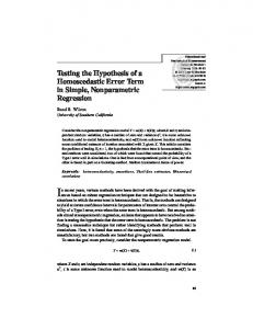
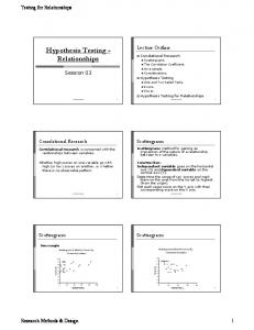
is formally shown that, for the single bad data case, the maximum normalized Lagrange multiplier points out the gross measurement, exactly as the maximum normalized residual also does. Preliminary tests applying the proposed problem formulation to process only gross analog measurements indicate that, assuming adequate redundancy levels, the entries of m are the most affected by the errors (recall that, in the case of topology errors, that conclusion applies to subvector o ). Therefore, it is feasible to extend the remaining steps of the method to allow the identi cation of multiple gross measurements. However, more research effort is needed to investigate the simultaneous occurrence of topology errors and gross measurements. The same applies to multiple bad data involving leverage points [21]. VII. S IMULATION R ESULTS The IEEE 24-bus test-system has been used to assess the performance of the proposed topology error identi cation method, which has been implemented considering a linear model for the network. The test system data and the description of its substations are given in reference [22]. As discussed in Section VI-B, topology error identi cation is conducted at the substation level, that is, only the “zoomed area” is considered. Therefore, in what follows attention will be focussed on substations (STs) corresponding to buses 14, 15, 16 and 24 of the original system presented in [22]. Different types of tests have been performed on the selected substations, considering the various forms of topology error: Exclusion Error, when a transmission line which is actually in service is inadvertently excluded in the system model. (Notice that this kind of error may be due to incorrectly reported status of either a single or two or more switching branches); Inclusion Error, when a transmission line is erroneously included in the state estimation model; By-Pass Error, when an incorrect by-pass of the substation is reported to the system model. The simulation results are separated into two groups, A and B. Figures 1 and 2 show the substation level model of the anomaly region, i.e. the zoomed area for Cases A and B, respectively. It is assumed that the ow at both ends of all transmission lines and the injection at each bus are monitored. Measurements have been simulated as noisy, with covariances around 2% of the true values. Structural and operational constraints are modeled as described in subsection II-A, and a priori values are considered as described in subsection II-B. The actual status of the switching branches and those among them for which the power ow is monitored are represented in Figures 1 and 2. The simulated topology errors for Cases A and B are described in Table I. The second and third columns of the table show the error type and the switching branches (SBs) involved in each test. The correct and simulated status for those devices are presented in the two remaining columns of Table I, where “0” and “1” represents open and closed status, respectively.

ST 15 ST 24 TL

B11

B10

B1

B4

B7

B2

B5

B8

B3

B6

B9

24

Closed switching branch 15

Load

to bus 16 to bus 21

to bus 3

Fig. 1.

Open switching branch

Zoomed Area for Case A

ST 16

ST 14

B8

B5

B2

B11

TL B1

B3

to bus 15

B4 14

B6

B9

B12

B77

B10

B13

Open switching branch Closed switching branch 16

to bus 11

Flow measurement

to bus 17

Load to bus 19

Fig. 2.

Zoomed Area for Case B

In what follows, fBk stands for the active power ow through circuit-breaker Bk : Also, Bk is the angular difference across switching branch Bk . A. Case A Two topology errors have been simulated to the network represented in Figure 1: an exclusion error involving a single breaker and an inclusion error as described in Table I. The results obtained with the proposed algorithm for both cases are described next. 1) Exclusion Error - Single Breaker: In this case, the status of switching branch B6 in Figure 1 is reported as open to the system model while its real status is closed. The criticality analysis in the rst step of the algorithm indicates that the network is observable and there are no critical operational constraint. Table II shows the critical sets determined for the simulated con guration. In the second step of the algorithm, t is initialized as 3:0. The results for this case is summarized in Table III. TABLE I S IMULATED T OPOLOGY E RRORS FOR C ASES A

Case A1

Error Type Exclusion (Single)

A2

Inclusion

B1

By-Pass

B2

Exclusion (Multiple)

SB

Correct

B6 B1 B7 B10 B8 B9 B10 B1 B5

1 0 0 0 1 0 1 1 1

AND

B

Status

Simulated 0 1 1 1 0 1 0 0 0

8

TABLE II

TABLE V

C RITICALITY A NALYSIS R ESULTS FOR C ASE A1

S USPECT S ET S ELECTION R ESULTS FOR C ASE A2

Critical Sets:

i = f:g = 0g; 2 =fP8 =0; fB2 = 0g; 3 =fP11 =0; fB6 = 0g 1 =fzP6 ; fB7

One can note that the status of switching branch B6 is the only one selected as suspect, what is con rmed by the cosine value shown in the second column of the Table. As a consequence, alternative hypothesis is restricted to the complementary closed status. The corresponding conditional probability value, shown in the last column of Table III, points out that the status of B6 is in fact closed.

Suspect Operational Constraints cos t = 3:0 B10 =0 B1 =0 B7 =0 B3 =0 0.99999 B9 =0 B6 =0 B8 =0 Component of 1 TABLE VI

H YPOTHESES T ESTING R ESULTS FOR C ASE A2 Suspect Set Hypotheses: Hi {B10 ; B1 ; B7 ; B3 ; B9 ; B6 ; B8 } f0 0 0 1 1 1 1g f1 0 0 1 1 1 1g f0 1 0 1 1 1 1g f0 0 1 1 1 1 1g

TABLE III S USPECT S ET S ELECTION R ESULTS FOR C ASE A1 Suspect Op. Constr. cos t = 3:0 fB6 = 0 0.99999

Suspect Set B6

P (H1 jz) 1.00000

H1 f1g

2) Inclusion Error: The operational condition shown in Figure 1 amounts to having the transmission line TL out of service. However, the status of switching branches B1 ; B7 and B10 are assumed closed in the con guration available for the state estimator. As a consequence, the transmission line is erroneously included in the network model. When the erroneous con guration is considered, those switching branches will be radially connected to the transmission line. As discussed in [12], a radial con guration involving a switching branch makes its status critical, that is, non-detectable. This criticality problem can be circumvented by extending the corresponding zoomed area (Figure 1) to prevent radial sections, as suggested in [23]. The results of the criticality analysis for the extended network are shown in Table IV. TABLE IV C RITICALITY A NALYSIS R ESULTS FOR C ASE A2

Critical Sets: 1 =fzP4 ; P18 =0; B7 =0;

2 =fP14 =0; fB4

B1 =0;

i

= f:g

B3 =0;

B8 =0; B10 =0g = 0; fB5 = 0g; 3 =fzf

B11

; fB11 = 0g

Taking into account the criticality analysis results, the suspect operational constraint shown in Table V are obtained. The cosine value is then computed by using Eq. (23). As also shown in the second column of Table VII, the cosine-test points out that all erroneous constraints have been selected as suspect. Therefore, the suspect set is composed by the corresponding switching branches shown in the last column of Table V. Finally, hypothesis testing is performed on the status of the suspect set. Table VI shows the alternative hypothesis for which the conditional probability value is found to be different from zero. These results show that the status of all suspect breakers are correctly identi ed by the alternative hypothesis with the largest conditional probability value.

Suspect Set B10 B1 B7 B3 B9 B6 B8

P (Hi jz) 0,99996 0,00001 0,00001 0,00001

B. Case B This subsection presents the results for Cases B1 and B2, related to Figure 2. 1) By-Pass Error: In Case B1 the status of switching branches B8 ; B9 and B10 are erroneously modeled as described in Table I. As a consequence, a wrong by-pass is considered in substation 16. Critical operational constraints are avoided by extending the zoomed area, as previously discussed. Table VII shows the results regarding the selection of suspect switching branches. The cosine value, also shown in the table, again con rms that all erroneous constraints have been selected. TABLE VII S USPECT S ET S ELECTION R ESULTS FOR C ASE B1 Suspect Operational Constraints cos t = 3:0 fB10 = 0 f B8 = 0 0.99999 B9 = 0 fB12 = 0 f B6 = 0

Suspect Set B10 B8 B9 B12 B6

The results obtained with the application of hypothesis testing indicate that conditional probability values are practically zero for all alternative hypothesis except for hypothesis H6 :{1 1 0 0 0}, whose probability value is found to be 1.0. Following the algorithm, the suspect status combination associated to hypothesis H6 is assumed as the correct con guration. This leads to the identi cation of the by-pass error involving B8 ; B9 and B10 . 2) Exclusion Error - Multiple Breaker: In Case B2 the status of switching branches B1 and B5 are reported as open while they are actually closed, erroneously excluding the transmission line TL represented in Figure 2. The operational constraints selected as suspect with the rst criterion ( t = 3:0) are shown in the rst column of Table VIII. The corresponding cosine value is shown in the second column of the table. The cosine test (cos < 1 cos ) is clearly not

9

satis ed, which means that not all erroneous constraints have been properly selected. Following the algorithm in subsection V-C, threshold t is reduced and the process is repeated until the cosine-test is satis ed. This is achieved when t =0:5: The third and fourth column of Table VIII show the suspect operational constraints and the cosine value in this case. The corresponding suspect switching branches are shown in the last column of the table. TABLE VIII S USPECT S ET S ELECTION R ESULTS FOR C ASE B2 Suspect Operational Constraints cos t =0:5 fB12 = 0 fB12 = 0 f B9 = 0 0.63752 fB9 = 0 f B5 = 0 f B1 = 0 t =3:0

cos 0.99999

Suspect SB B12 B9 B5 B1

Hypothesis testing is then performed on the suspect set. The conditional probability value is found to be equal to 1.0 for alternative hypothesis H8 :{0 0 1 1} and practically zero for all remaining alternative hypothesis. One can easily verify that hypothesis H8 represents the correct status combination for the suspect set of switching branches. Table IX shows the hypothesis testing results for cases B1 and B2, discussed in this subsection. TABLE IX H YPOTHESES T ESTING R ESULTS FOR C ASE B Case B1 B2

Error Type By-Pass Exclusion

Hypotheses H6 :{1 1 0 0 0} H8 :{0 0 1 1}

P (Hi jz) 1.0000 1.0000

C. Comparison of Computational Performance with Respect to the Re-Estimation Approach [12] This subsection quantitatively compares the computational performances of the proposed topology error identi cation method and the approach based on repeated runs of the state estimator employed in [12]. In the former case, the performance index , denoted by tBayes , corresponds to the cpu time to run the base case state estimation and to determine the conditional probabilities for all alternative status con gurations. As for the method used in [12], the de nition of a computational performance index is not so straightforward, since the number of runs of the state estimator that are performed until reaching the correct combination of circuit breaker statuses is a random variable whose value is unknown in advance. Since the maximum number of trials is 2nsb , where nsb is the number of suspect breakers, we assume that, on average, the correct status con guration is reached in half of that number, that is, in 2nsb 1 trials, nsb > 1. In addition, it has been veri ed that the cpu time to perform a single state estimation, testim , does not vary signi cantly when the hypotheses vary, so that the computational performance index for the re-estimation method is de ned as tre est = 2nsb 1 testim (31)

Table X presents the ratio between the two methods' performance indices for all cases simulated in the previous subsections. Results have been obtained on a 800 M Hz PC, using MATLAB version 6.0. It can be seen that, even for the case of a single alternative hypothesis, the Bayesian approach outperforms the re-estimation method, being almost twice as fast. The speed-up provided by the proposed method tends to increase as the number of suspect circuit breakers (and consequently the number of alternative hypothesis) grow, as also illustrated by the results presented in Table X. TABLE X C OMPUTATIONAL P ERFORMANCE C OMPARISON Error Type Exclusion (Single) Exclusion (Multiple) By-Pass Inclusion

nsb 1 4 5 7

tBayes = tre 0:542 0:190 0:139 0:120

est

VIII. C ONCLUSIONS This paper presents a methodology for detecting and identifying topology errors in generalized state estimation. It is centered on the use of Bayesian-based hypothesis testing, which provides conditional probabilities for hypothesis made about the status of suspect devices. To enhance both the performance and the ef ciency of the proposed approach, two additional procedures are incorporated in the identi cation process. A geometric test ensures that all devices with wrong status are included in the suspect set. In addition, criticality analysis allows that topology error identi cation proceeds even when the error involves members of critical sets. The proposed methodology has been tested by using the IEEE 24-bus test system. Different types of topology errors involving substations with different layouts have been considered. The results con rm the ef ciency of the suspect set determination and the robustness of the hypothesis testing identi cation. The method has been able to provide correct answers even when measurement redundancy is low. In those cases, critical constraints and critical sets tend to degrade the normalized Lagrange multipliers sensitivity, and consequently the identi cation process is subject to more severe conditions.

ACKNOWLEDGMENTS Kevin A. Clements acknowledges the support from National Science Foundation, under Grant ECS-9810288. Antonio Simões Costa thanks the support of the Brazilian National Research Council (CNPq). Elizete Lourenço acknowledges the nancial support of the Brazilian Agency for the Improvement of High Education (CAPES).

R EFERENCES [1] A. Bose and K. A. Clements. “Real Time Modeling of Power Networks”. Proceedings of the IEEE, 75(12):1607–1622, Dec. 1986. [2] L. Mili, T. Van Cutsem, and M. Ribbens-Pavella. “Hypothesis Testing Identi cation : A New Method for Bad Data Analysis in Power System State Estimation”. IEEE Trans. on Power Apparatus and Systems, 103(11):3239–3252, Nov. 1984.

10

[3] R. L. Lugtu, D. F. Hackett, K. C. Liu, and D. D. Might. “Power System State Estimation: Detection of Topological Errors”. IEEE Trans. on PAS, 99(6):2406–2412, Nov./Dec. 1980. [4] A. Simões Costa and J. A. Leão. “Identi cation of Topology Errors in Power System State Estimation”. IEEE Trans. on Power Systems, 8(4):1531–1538, November 1993. [5] F. F. Wu and W. E. Liu. “Detection of Topology Errors by State Estimation". IEEE Trans. on Power Systems, 4(1):176–183, February 1989. [6] N. Singh and H. Glavitsch. “Detection and Identi cation of Topological Errors in On Line Power System Analysis". IEEE Trans. on Power Systems, 6(1):324–331, February 1991. [7] S. G. Souza. “Identi cação de Erros de Topologia em Sistemas de Potência Utilizando Técnicas de Sistemas Especialistas”. Diss. Mestrado - Universidade Federal de Santa Catarina - Florianópolis, SC, Brasil, Aug. 1995. [8] A. Monticelli and A. Garcia. “Modeling Zero Impedance Branches in Power System State Estimation". IEEE Transactions on Power Systems, 6, 1991. [9] A. Monticelli. “Modeling Circuit Breakers in Weighted Least Squares State Estimation". IEEE Trans. on Power Systems, 8(3):1143–1149, August 1993. [10] O. Alsaç, N. Vempati, B. Stott, and A. Monticelli. “Generalized State Estimation”. IEEE Trans. on Power Systems, 13(3):1069–1075, Aug. 1998. [11] A. Simões Costa, E. M. Lourenço, and K. A. Clements. “Power System Topological Observability Analysis Including Switching Branches”. IEEE/PES Trans. on Power System, 17(2):250–256, May. 2002. [12] K. A. Clements and A. Simões Costa. “Topology Error Identi cation using Normalized Lagrange Multipliers”. IEEE Trans. on Power Systems, 13(2):347–353, May 1998. [13] K. A. Clements and P. W. Davis. “Multiple Bad Data Detectability and Identi ability: a Geometric Approach”. IEEE Transaction on Power System, 3(4):461–466, Nov 1985. [14] K. A. Clements, A. Simões Costa, and A. Agudelo. “Bayesian Estimation to the Identi cation of Undisclosed Bilateral Transactions”. PMAPS Conference, Madeira, Portugal, 2000. [15] E. M. Lourenço. “Observability Analysis and Topology Error Identication in the Generalized State Estimation”. Ph.D. thesis, Electrical Engineering Graduate Program, Universidade Federal de Santa Catarina, Brazil, (in Portuguese) 2001. [16] E. M. Lourenço, K. A. Clements, and A. J. A. Simões Costa. “Geometrically-Based Hypothesis Testing for Topology Error Identi cation”. 14th Power System Computation Conference, Seville, Spain, Jun. 2002. [17] L. Colzani. “Determining Bad Data Pockets for Topology Error Identi cation in Power System state estimation”. Master's thesis Universidade Federal de Santa Catarina, Brazil, Feb. 2001. [18] A. Monticelli. “The Impact of Modeling Short Circuit Branches in State Estimation". IEEE Trans. on Power Systems, 8(1):364–370, Feb 1993. [19] J. Pereira, V. Miranda, and J. T. Saraiva. “A Comprehensive State Estimation Approach for EMS/DMS Applications”. IEEE Power Tech Conference, Budapest, Hungary, 1999. [20] A. Abur, H. Kim, and M. K. Celik. “Identifying the Unknown Circuit Breaker Statuses in Power Networks". IEEE Trans. on Power Systems, 10(4):2029–2037, Nov. 1995. [21] L. Mili, V. Phaniraj, and P. J. Rousseeuw. “Least Median of Squares Estimation in Power Systems”. IEEE Transactions on Power Systems, 6(2):511–523, May 1991. [22] R. Billinton, P. K. Vohra, and S. Kumar. “Effect of Station Originated Outages in a Composite System Adequacy Evaluation of the IEEE Reliability Test System”. IEEE Power Apparatus and Systems, 104(10):2249–2656, Oct. 1985. [23] E. M. Lourenço, A. J. A. Simões Costa, and K. A. Clements. “A Hybrid Probabilistc/Topological Approach to Topology Error Identi cation in Power System Real-Time Modeling”. 7a PMAPS Conference, Naples, Italy, pages 105–110, Sep. 2002.

Elizete M. Lourenço (Member, IEEE) received her degree in Electrical Engineering, as well as her M.Sc. and Ph.D. degrees in Electrical Engineering from Federal University of Santa Catarina, Brazil, in 1992, 1994 and 2001, respectively. She spent the 2000 academic year in Worcester Polytechnic Institute, USA, working in her Ph.D research. Since 1995 she is a Faculty member with the Department of Electrical Engineering at Federal University of Paraná,

Brazil. Her research interests are in the area of computer methods for power systems operations. Antonio Simões Costa (Senior Member, IEEE) received his degree in Electrical Engineering from Federal University of Pará, Brazil, in 1973, and M.Sc. and Ph.D. degrees in Electrical Engineering from Federal University of Santa Catarina (UFSC), Brazil, in 1975, and University of Waterloo, Canada, in 1981, respectively. Since 1975 he is with UFSC's Department of Electrical Engineering . His research interests are concerned with computer methods for power systems operation and control. Kevin A. Clements (Fellow, IEEE) received the B.S. degree in Electrical Engineering from Manhattan College, Bronx, NY, in 1963, and the M.S. and Ph.D. degrees from the Polytechnic Institute of Brooklyn, NY, in 1967 and 1970, respectively. In 1970 he joined the Electrical and Computer Engineering Department at Worcester Polytechnic Institute, Worcester, MA, where he is presently a Professor. His research interests include monitoring and control of electric power systems, power system stability, and methods for large-scale systems.