Bayesian Calibration for Transient Energy Simulation Model
Dong-HyunLee1,Young-JinKim2, and Cheol-Soo Park1,* 1
Department ofu-City Design and Engineering, SungKyunKwan University, South Korea. 2 Departmentof Architectural Engineering,SungKyunKwanUniversity, South Korea.
ABSTRACT Building simulation has become increasingly important because of its capability to assess potential energy efficiency savings in buildings. In the simulation modellingprocess, many assumptions and simplifications are required and many uncertain inputs are also involved. The aforementioned issues may cause a significant discrepancy between a reality and prediction. With this in mind, this paper investigatesapplicability of a Bayesian calibration technique to a transient simulation model. This will improve prediction accuracy and reduce uncertainty. The Bayesian calibration is a way to estimate the posterior distribution based on the quantified prior distribution.For sampling uncertain inputs, MCMC(Markov Chain Monte Carlo) method was applied in our study. One of the MCMC methods, DRAM(Delayed Rejection Adaptive Metropolis) was employed. This paper addresses Bayesian calibration, uncertainty analysis, and risk analysis for whole-building building energy simulation modelling(EnergyPlus). For this study, an office building was selected and 28 unknown inputs were identified. The Bayesian calibration was conducted in three steps: (1) determination of prior probability distributions for uncertain inputs, (2) formulation of likelihood functions,and (3)MCMC method for posterior distributions. Lastly, Coefficient of Variation of the Root Mean Squared Error (CVRMSE, ASHRAE Guide line14) was used for the validation of the approach. In the paper, the following is discussed: (1) posterior distributions of inputs against their prior distributions, (2)results of Bayesiancalibration for the model, and (3) advantages of Bayesian calibration for dynamic simulation model. KEYWORDS Bayesian,Markov Chain Monte Carlo,dynamic simulation,model calibration INTRODUCTION Building simulation has been attributed to reduction of building energy use.The simulation tools can present predicted results such as energy use, thermal comfort, indoor air quality, etc.However, modellingassumptions and simplifications as well as *
Corresponding author email:
[email protected]
uncertainty inputs, which are involved in the process of performance simulation, are believed to cause a gap between simulation prediction and measurement. Many studies presenteddiscerniblediscrepancies between the building simulation results and the real measurements (IBPSA, 1987-2011).In the light of this perspective, the calibration technique is a necessity to estimate uncertaininputs and to cancel out knowingly or unknowingly unmodeledor simplifieddynamics. This paper addressesapplicability of the Bayesian calibration technique to a transient energy simulation model (EnergyPlus v.6.0) and describesits impacts and advantages. For this study, the Bayesian calibration method was conducted in three steps: (1) determination of prior probability distributions for uncertain inputs based on the literature, (2) formulation of likelihood functions,and (3)Markov Chain Monte Carlo(MCMC) for posterior distributions. SIMULATION MODEL A 5-storeysample office building located in Seoul, Korea was selected for this study. Figure 1 shows the energy simulation model consisting of five thermal zones (four perimeter zones and one interior zone) in each floor. A total floor area is 6,125 m2, and a ratio of window area to wall area is 35.7%. As for the HVAC system, “IdealLoadAirSystem (or purchased air)” was applied. The IdealLoadAirSystem is used to calculate heating and cooling loads without taking into account equipment efficiency or performance (Ellis &Torcellini, 2005). For a building energy performance tool, EnergyPlus 6.0 developed by Department of Energy (DOE) was utilized.The 28unknowninputs (Macdonald, 2002; ASHRAE, 2009; Hopfe, 2009; Doe, 2010) in the EnergyPlus modelwere selected in this study (c.f.Table2 Prior distributions).The selected unknown inputs were composed of normal distribution with mean (μ) and standard deviation (σ). The unknown inputs were assumed independent of each other.
Figure 1.Targetbuilding (Display: OpenStudio) BAYESIAN CALIBRATION There are typically three ways for calibrating the simulation model: (1) manual calibration (‘trial and error’ or ‘rule of thumb’ approach: selection of any input based on expertise or intuition change the value of it see the result and repeat until it is
satisfactory), (2) deterministic optimization (use of an optimization function that minimizesa difference betweenthe prediction and the measurement), and (3) Bayesian calibration (stochastic optimization).In this study, the authors selected the Bayesian calibration for reducing uncertainty of theunknown inputs inherited inthe simulation model, rather than a best-fit one.The Bayesian calibration, which is based on the Bayes’theorem as shown in equation (1), is an effective stochasticapproach for finding a distribution of solutions in each unknowninput (θ)in the simulation model (m) given observed data (y).To calculate on posterior distribution (P(θ|y, m)), prior distribution (π(θ, m)) and likelihood function P(y,m| θ)must be taken into account. The likelihood function is the probability of the data for thegiven unknowninputs (θ).Observation (y(x)) formulated by model outputs η(x,θ) at known inputs (x), unknown inputs (θ), and observation error (ℇ(x)) as the Gaussian process model defined by Kennedy and O’Hagan (2002) (equation (2)). P(θ|y,m)∝P(y,m|θ)ⅹπ(θ, m)
(1)
y(x) = η(x,θ)+ε(x)
(2)
Due to lack of real observed data (e.g. electric or gas consumption), we used simulation outputs (monthly total energy load), which were generated based randomly selected inputs and climate file (*.epw) in 2009-2011 years, as observed data.The observed data in 2009-2010 years were used for Bayesian calibration. On the other hand, the observed data in 2011 year was used for validation of the calibrated simulation model data.Table 1 shows observation results for the sample office building (Figure 1). Table 1.Observed data(kWh/m2) For calibration Month Year2009 Year2010 1 5.85 6.57 2 3.70 4.58 3 3.92 4.01 4 4.64 3.27 5 8.35 5.87 6 10.18 8.98 7 9.71 9.13 8 12.04 10.71 9 9.07 8.13 10 6.33 5.53 11 4.23 3.92 12 5.19 5.16
For validation Year2011 7.50 3.88 3.70 3.81 7.38 9.21 8.95 10.04 8.96 5.57 4.42 4.95
The authors adopted Metropolis-Hastings MCMC chain using multivariate Gaussian proposal distribution. The Metropolis-Hastings algorithm is a convenient sampling technique in MCMC method. The MCMCis Monte Carlo integration using Markov
Chains (Gilks et al, 1995).To runs MCMC chain, the time period wasselected as 4,000 iterations, and the time period for burn-in phase was selected as the first 10%of a chain(Van Oijen et al, 2005). The burn-in phase will discard a portion of the initial iterations for drawing right searches in input space. RESULTS AND VALIDATION Figure 2 shows Probability Density Function (PDF) of the four prior and posterior distributions. The four inputs in Figure 2 were randomly selected. The distributions represented in blue are the prior distribution, and the posteriors are shown in red.Table 2 shows mean and standard deviation of 28 unknown inputs before and after Bayesian calibration. As shown in Table 2 and Figure 2, there is a significant difference between prior and posterior distributions. If the prior data are informative, the posterior distributions will be narrower, and more sharply peaked than the prior distribution, indicating that uncertainty is reduced. If initial inputs were completely informative, and have low error, posterior distributions have strong robustness and are sharply peaked. For the infiltration rate (Figure 2(a)), the posterior distribution shifts to the lower bound by 0.23. This update means that air tightness in the calibrated model is less than that in the uncalibrated model. For the activity level (Figure 2(b)), the posterior distribution is toward lower bound while its shape maintains the same as the prior distribution. This shift indicates that the mean of activity level for the calibrated model is smaller than that for the uncalibrated model. Regarding the lighting level (Figure 2(c)), the posterior distribution does not shifted much from the prior distribution. On the contrary, for the conductivity of a brick (Figure 2(d)), the posterior distribution is shifted the most. This inputs increase approximately by 36% from the prior mean value. 0.16
(a) Prior Distribution (b) Posterior Distribution
20
(a) Prior Distribution (b) Posterior Distribution
0.12
PDF
PDF
15
10
0.08
0.04
5
0
-0.4
-0.2
0
0.2 0.4 0.6 0.8 1 Infiltration (Airchanges/Hour)
1.2
1.4
0
1.6
60
80
(a) Infiltration (ID-18) 0.35
120 140 Activity Level (W/m2)
160
180
(b) People (ID-23) 2.4
(a) Prior Distribution (b) Posterior Distribution
(a) Prior Distribution (b) Posterior Distribution
1.8
PDF
0.25
PDF
100
1.2
0.15
0.6 0.05 0
0
5
10
25 15 20 2 Lighting Level(W/m )
(c) Lighting (ID-24)
30
35
0
-0.5
0
0.5 1 1.5 2 Brick Conductivity(W/m*k)
2.5
3
3.
(d) Brick (ID-4)
Figure 2.Prior distribution and Posterior distribution (randomly selected 4 out of 28)
Table 2.Results of Bayesian calibration
1 2
Prior distribution Mean St.dev 0.43 0.15 1488 501
Specific Heat(J/kg∙K) Conductivity(W/m∙K) Density(Kg/m3 ) Specific Heat(J/kg∙K) Conductivity(W/m∙K) Density(Kg/m3 ) Specific Heat(J/kg∙K) Conductivity(W/m∙K) Density(Kg/m3 ) Specific Heat(J/kg∙K) Conductivity(W/m∙K)
3 4 5 6 7 8 9 10 11 12 13
958 1.25 2000 840 1.68 2310 840 0.04 38 1072 0.93
109 0.35 33 90 0.54 225 90 0.01 27 298 0.41
972.64 1.70 1980.01 892.43 0.95 2329.59 829.61 0.04 3.92 969.70 1.20
70.29 0.17 17.24 22.14 0.19 72.03 9.47 0.01 4.52 152.07 0.04
Density(Kg/m3 )
14
1610
436
1830.66
159.32
15 16 17 18 19
818 1.72 0.17 0.50 21.50
89 0.17 0.02 0.17 2.15
803.18 1.67 0.17 0.27 22.64
48.43 0.095 0.00 0.02 0.47
20
27
2.70
28.20
0.88
21 22 23 24 25 26 27 28
0.22 0.48 125 18.22 0.42 0.18 16.15 0.30
0.11 0.05 12.50 3.64 0.04 0.02 3.23 0.03
0.17 0.50 115.07 17.12 0.49 0.19 15.26 0.32
0.03 0.03 2.82 1.19 0.01 0.01 1.24 0.01
Input variables Plaster Board
Brick Medium Weight Concrete Insulation
Acoustic Tile Window Infiltration
Conductivity(W/m∙K) Density(Kg/m3 )
Specific Heat(J/kg∙K) U-Factor(W/m2∙K) SHGC AirChanges per Hour
Heating (℃) Set point temperature Cooling (℃) Person/area Fraction radiant (%) People Activity level(W/m2 ) Lighting level(W/m2 ) Fraction radiant (%) Lighting Fraction visible (%) Watt/area(W/m2 ) Equipment Fraction radiant (%)
ID
Posteriordistribution Mean St.dev 0.47 0.06 1178.79 253
To validate for Bayesian calibration, Coefficient of Variation of the Root Mean Squared Error(CVRMSE) value was used. The simulation model can be consideredvalid, in the case where the CVRMSE values of the calibrated models is equal or less than 15% (ASHRAE,2002).In this study, Latin Hypercube Sampling (LHS) method was applied to obtain 100 samplings, with which calibrated and uncalibrated modelscould be compared.100 CVRMSE valueswere calculated from the simulated results.Energy use from the calibrated and the uncalibratedwere respectively checked by validating the 2011-year-weather data100 times.As shown in Table3, an averageof 100 CVRMSE valuesfor energy use fromthe uncalibrated model was40.21%. On the other hand, an averageof 100 CVRMSE valuesfor prior energy
use from the calibrated model was9.94%.An average of 100 CVRMSE valuesforposterior energy use from the calibrated model ranged within the confidence level.It indicates that stochastic calibration enhances the accuracy of model. Table 3.Validation results for uncalibrated and calibrated model (Unit: %) Uncalibrated energy use Calibrated energy use CVRMSE vs.Observed energy use vs.Observed energy use Average 40.21 9.94 Within 15% Probability 14.27 82.55 Table 4 represents each average energy use fromthe uncalibrated(b) and the calibrated model(c).The difference (|(a) – (c)|)between the 2011-observed energy use and an average energy use from the calibrated modelis smaller thanthe difference (|(a) – (b)|) between the 2011-observedenergy use and an average energy use from uncalibrated model. It means that uncertainty of the uncalibratedmodelreduced, approaching to2011 observed energy use. Table 4.Average energy use for the uncalibratedandthe calibratedmodel (Unit: kWh/m2) 2011-Observed Uncalibrated Calibrated Month |(a) – (b)| |(a) – (c)| energy (a) Model(b) Model(c) 1.47 0.04 1 7.50 8.97 7.54 0.27 0.08 2 3.88 4.15 3.96 0.19 0.12 3 3.70 3.89 3.82 0.34 0.09 4 3.81 4.15 3.90 1.20 0.05 5 7.38 8.58 7.43 1.70 0.04 6 9.21 10.91 9.25 1.97 0.04 7 8.95 10.92 8.99 2.35 0.13 8 10.04 12.39 10.17 1.60 0.06 9 8.96 10.56 9.02 0.62 0.04 10 5.57 6.19 5.61 0.42 0.11 11 4.42 4.84 4.53 0.36 0.04 12 4.95 5.31 4.99 Total
78.37
90.85
12.48
79.21
0.84
In Figure3, monthly average energy uses from the uncalibrated and the calibrated model are shown in a boxplot. As shown in Figure3, the uncalibrated simulation model is distributed in a wide range of energy use. On the other hand, the calibrated simulation model is distributed in a narrower range than the uncalibrated model. It means that the unknown inputs’ uncertainty reduced.It shows advantage of stochastic calibration.
Figure 3.Energy use(uncalibratedvs.calibratedvs.observed) CONCLUSION This study presents an example of Bayesian calibration for the transient simulation model.In this study, the posterior distribution can be estimated by usingquantification of prior knowledge and reflection on observed data. The main purpose of this study is to increase model accuracy andto validatean energy simulation model.As a result of Bayesian Calibration, the unknown inputs of anenergy simulation modelhave the mean and the Standard deviation for posterior distributions. The calibrated model and the uncalibrated model have difference in the mean and the Standard deviation. The calibrated model was superior to the uncalibrated model in terms of robustness.It was attributed to Bayesian calibration.From the validation results of energy simulation model, it is shown that CVRMSE of the calibrated modelwas better than that of the uncalibrated model.Thus, withcomparing the energy use in after-calibration and before-calibration, the energy useinafter-calibration was stochastically closer to the observed data. Bayesian calibration enhances the reliability and accuracy for a transient energy model. ACKNOWLEDGEMENT This work is financially supported by the Korea Minister of Ministry of Land, Transport and Maritime Affairs (MLTM) as “U-City Master and Doctor Course Grant Program”. This research is supported by a grant (11 High-tech Urban G02) from High-tech UrbanDevelopmentProgramfunded by Ministry of Land, Transport and Maritime Affairs ofKorean government. REFERENCES ASHRAE. 2002.ASHRAE Guideline 14-measurement of energy and demand savings. American Society of Heating, Refrigerating, and Air-Conditioning Engineers, Atlanta, GA.
ASHRAE. 2009. ASHRAE Handbook Fundamentals, Atlanta: American Society of Heating, Refrigerating, and Air-Conditioning Engineers, Inc. DOE. 2010.EnergyPlus6.0 Input/Output Reference: The Encyclopedic Reference to EnergyPlus Input and Output, US Department Of Energy Ellis, P.G, and Torcellini, P.A. 2005.Simulating Tall Buildings Using EnergyPlus, Proceedings of the 9th IBPSA Conference, August 15-18, Montreal, Canada, pp. 279-286 Gilks, W. R, Richardson, S, and Spiegelhalter, D. 1995.Markov Chain Monte Carlo in Practice, Chapman and Hall. Hopfe. 2009. Uncertainty and sensitivity analysis in building performance simulation for decision support and design optimization. PhD thesis,Technische Universiteit Eindhoven. Heo, Y.S, Choudhary, R, and Augenbroe, G. 2012. Calibration of building energy models for retrofit analysis under uncertainty, Energy and Buildings, Vol. 47, pp. 550-560 IBPSA. 1987-2011. Proceedings of the IBPSA(International Building Performance Simulation Association) conference ('87. '91, '93, '95, '97, '99, '01, '03, '05, '07, '09, ‘11)
Kennedy, M.S, andO'Hagan, A. 2002. Bayesian calibration of computer models, Journal of the Royal Statistical Society: Series B, Vol. 63, pp. 425-464 Macdonald, I.A. 2002. Quantifying the effects of uncertainty in building simulation,Ph.D. thesis, University of Strathclyde, Scotland. Van Oijen, M,Rougier, J, and Smith, R. 2005, Bayesian calibration of process-based forest models: bridging the gap between models and data, Tree Physiology,Vol. 25, pp. 915–927