Bayesian classification of catchments using spatial data: a first step to improved modelling of catchment effects on stream ecological condition 1
Webb, J.A., 2N.R. Bond, 2S.R. Wealands, 2,3R. Mac Nally, 1M.R. Grace and 2G.P. Quinn
Monash University & CRC for Freshwater Ecology, Clayton, Vic. Water Studies Centre, Dept. of Chemistry, 2Dept. of Biological Sciences, 3Australian Centre for Biodiversity: Analysis, Policy, Management, E-Mail:
[email protected]
1
Keywords: classification, Bayesian models, spatial data, Murray Darling Basin, catchment, physiography EXTENDED ABSTRACT A major challenge facing freshwater ecologists and managers is the development of models that link stream ecological condition to catchmentscale effects, such as land use. Previous attempts to make such models have followed two general approaches. The bottom-up approach employs mechanistic models, which can quickly become too complex to be useful. The top-down approach employs empirical models derived from large data sets, and has often suffered from large amounts of unexplained variation in stream condition. We believe that the lack of success of both modelling approaches may be at least partly explained by scientists considering too wide a breadth of catchment type. Thus, we believe that by stratifying large sets of catchments into groups of similar types prior to modelling, both types of models may be improved. This paper describes preliminary work using a Bayesian classification software package, ‘Autoclass’ (Cheeseman and Stutz 1996) to create classes of catchments within the Murray Darling Basin based on physiographic data. Autoclass uses a model-based classification method that employs finite mixture modelling and trades off model fit versus complexity, leading to a parsimonious solution. The software provides information on the posterior probability that the classification is ‘correct’ and also probabilities for alternative classifications. The importance of each attribute in defining the individual classes is calculated and presented, assisting description of the classes. Each case is ‘assigned’ to a class based on membership probability, but the probability of membership of other classes is also provided. This feature deals very well with cases that do not fit neatly into a larger class. Lastly, Autoclass requires the user to specify the measurement error of continuous variables. Catchments were derived from the Australian digital elevation model. Physiographic data were
1497
derived from national spatial data sets. There was very little information on measurement errors for the spatial data, and so a conservative error of 5% of data range was adopted for all continuous attributes. The incorporation of uncertainty into spatial data sets remains a research challenge. The results of the classification were very encouraging. The software found nine classes of catchments in the Murray Darling Basin. The classes grouped together geographically, and followed altitude and latitude gradients, despite the fact that these variables were not included in the classification. Descriptions of the classes reveal very different physiographic environments, ranging from dry and flat catchments (i.e. lowlands), through to wet and hilly catchments (i.e. mountainous areas). Rainfall and slope were two important discriminators between classes. These two attributes, in particular, will affect the ways in which the stream interacts with the catchment, and can thus be expected to modify the effects of land use change on ecological condition. Thus, realistic models of the effects of land use change on streams would differ between the different types of catchments, and sound management practices will differ. A small number of catchments were assigned to their primary class with relatively low probability. These catchments lie on the boundaries of groups of catchments, with the second most likely class being an adjacent group. The locations of these ‘uncertain’ catchments show that the Bayesian classification dealt well with cases that do not fit neatly into larger classes. Although the results are intuitive, we cannot yet assess whether the classifications described in this paper would assist the modelling of catchmentscale effects on stream ecological condition. It is most likely that catchment classification and modelling will be an iterative process, where the needs of the model are used to guide classification, and the results of classifications used to suggest further refinements to models.
1.
INTRODUCTION
One of the primary challenges currently facing freshwater ecologists and managers is that of modelling catchment-scale effects (e.g. patterns of land use) on ecological condition of rivers and streams. Although it has long been realized that aquatic ecosystems are inextricably linked to their catchments (e.g. Borman and Likens 1979), attempts to explicitly model the effects of catchment-scale influences on waterways have met with limited success (Allan 2004). Attempts to model the link between the catchment and stream have historically tended to follow two paradigms. The first of these is the ‘bottom up’ approach, in which mechanistic models based on theories of ecosystem function are employed. Such models are usually most effective if the system can be simplified into few components – both in terms of catchment scale influences, and the ecological response being examined. Attempts to create generic models quickly become too complex to be parameterised, and thus cannot be used in a predictive sense. The second approach to modelling is the ‘top down’ approach where statistical models are developed between catchment-scale effects and ecological condition, with little attempt to impose structure on the models beyond those mandated by the statistical approach being used. Despite some successes, the amount of variation in ecological condition explained by these statistical models is often insufficient to draw unambiguous conclusions about the direct impacts of land-use change (Allan 2004). We argue that the limited success of both bottomup and top-down modelling may at least be partly explained by researchers simultaneously considering too wide a breadth of catchment type. As stated above, generic conceptual models of catchment-scale influences on stream condition are too complex to be used. Moreover, it is reasonable to suppose that influences of a given catchment-scale variable on a particular aspect of stream ecology may vary with other catchment characteristics, but only a very complex model could incorporate such interactions. In contrast, by considering a wide range of catchment types simultaneously, the top down model may be introducing too much unexplained variation, as the differences in catchments moderate the ecological response to a given stressor. We hypothesise that by stratifying sets of catchments into different types prior to modelling, both bottom-up and top-down approaches might be improved. Bottom up models would benefit from a reduced requirement for complexity, as models could be built for the particular dominant
1498
catchment-scale effects. The models would also benefit from knowledge of the particular type of stream to which the model was being applied. Top down models would benefit due to a reduction in the amount of unexplained variation, as above. The question then is how such groups of catchments should be formed. In this paper, we describe the application of a Bayesian classification software package ‘Autoclass’ to define classes of catchments within the Murray Darling Basin, Australia using physiographic data derived from national-coverage spatial data sets. 2.
BAYESIAN CLASSIFICATION WITH AUTOCLASS
There are dozens of different methods that can be used to classify cases based on multivariate data, and classification is an area of active and diverse research. All methods have strengths and weaknesses, and the ‘best’ choice of a classification method is determined largely by the application in question. For this exercise, we chose Autoclass (Cheeseman and Stutz 1996, Hanson et al. 1991), and in particular Autoclass C for MS-DOS. A brief description of how this package works, along with the features that attracted us to it, follows. Autoclass employs a model-based classification method, in that it attempts to fit statistical models to the data to derive classes. Specifically, Autoclass treats the distribution of data for a specific attribute (e.g. catchment area) as a mixture of K distributions, where K is the number of classes. The user can specify the number of classes, or the software can operate in ‘unsupervised’ mode, where both K and the membership of each class are determined by the data. For a Bayesian model, overall fit to the data is measured by the posterior probability of the model. Autoclass searches randomly over the space of possible classifications from multiple starting points, replacing its ‘best’ choice with the new classification if the estimated posterior probability for the new classification is greater. When using non-informative prior distributions for model parameters, this method effectively compromises between model complexity and model fit, providing the most parsimonious solution to the classification problem (Cheeseman and Stutz 1996). Following a search, the system gives basic information for the 10 most likely classifications found, including the number of classes in each, and the posterior probability that each classification is the ‘correct’ one (i.e. the probability of the classification given the data at hand). Detailed reports can be generated for any number of these classifications. The probabilities
reported allow the user to determine whether the best classification found is sufficiently more probable than other classifications to render them of no interest, or whether the two or three most likely classifications are worthy of consideration due to their similar posterior probabilities. Autoclass models several attribute types, and allows for both continuous and categorical data. In this study, the various attributes were modelled as either continuous lognormal variables (following loge transformation), or as multinomial variables. Some implementations of Autoclass allow a wider range of attribute types (Cheeseman and Stutz 1996). The software also allows groups of continuous variables to be defined as a correlated set, and classifications then are based on differences in the relationship between the variables, rather than on the distributions of the individual variables (Hanson et al. 1991). As output, Autoclass provides information on the relative strength of each of the classes found, and on how far each class diverges from the global distribution of data. Each case is ‘assigned’ to a class, based on membership probability, but the user is also supplied with membership probabilities for other classes. This is a particular strength of the approach, because it deals well with isolated cases that do not fit neatly into one larger class. Information is also presented on the importance of the individual attributes – both in terms of their overall effect on the classification, and their effect on each class. The importance of each attribute is ranked based on the Cross Entropy or KullbackLeibler distance (Cover and Thomas 1991) between the modelled class-level distribution of an attribute and the global distribution of that attribute. The Kullback-Leibler distance (hereafter KLD) is a convenient measure of distance between probability distributions, because it takes into account both differences in the central tendencies of the distributions (e.g. mean) and also the variability of the distribution (e.g. standard deviation). It is also calculable for both continuous and discrete distributions. The KLDs for the individual attributes in a class show which attributes were important in distinguishing this class from the global distribution. Between classes, the KLDs for a particular attribute give a rank ordering of how far from ‘average’ each class is for that attribute. Along with the KLD, Autoclass supplies information on the modelled class distribution for each attribute, which can then be compared to the global distribution for descriptive purposes. As a fully Bayesian approach, Autoclass explicitly deals with and presents uncertainties for all
1499
aspects of the classification. Moreover, the software requires the user to specify a measurement error for each of the continuous attributes in the classification. Thus, although the data may list the length of an object at 10 m, the software treats this datum as say 10±0.5 m. The practical consequence of specifying uncertainty is that a relatively uncertain variable has less influence on a classification than a more certain variable, even if the two have the same distribution of data values. Although being forced to specify uncertainty may initially appear as a weakness (or at least an inconvenience) of the software, it is really a strength. We are never completely certain of measured data values, and if information on our certainty or lack of it is included in statistical analyses, the results will be more robust. 3.
SPATIAL DATA
The aim of this exercise was to classify catchments within the Murray Darling Basin (MDB). To obtain catchment boundaries within the basin, a digital elevation model (DEM) was used. The latest version of the 9” DEM of Australia (Hutchinson et al. 2000), and the associated flow directions were provided by the Centre for Resources and Environmental Studies. This elevation model uses the ANUDEM interpolation algorithm (Hutchinson 1989) to enforce drainage structure and produce gridded estimates of elevation. This is the underlying dataset to all derived catchment boundaries, and has an approximate cell size of 250 m. Using standard terrain analysis functions in ESRI ArcGIS 9.0 (ESRI 2004), catchments of different orders were defined and their scale characterized using Strahler stream ordering (Strahler 1957). To define the first order streams for this study, a threshold accumulation area of 6 km2 was used, which coincides approximately with headwater streams in 1:250,000 topographic mapping of Australia. For this demonstration of the classification results, we confine our attention to order 4 catchments. Under the catchment definition, some areas of the MDB were excluded from consideration (see Figure 1). The classification described in this paper was based on physiographic characteristics of the catchments. The attributes described for each catchment were generated from either the DEM, the Climatic Atlas of Australia (BOM 2003), or from the MDB Soil Information Strategy (Bui and Moran 2003). A complete list of attributes recorded for each catchment is given in Table 1. A deliberate decision was made to focus on variation in attribute values as much as mean values.
Table 1. Catchment Attributes used in the classification
but the effects of multiple cells in the catchment will again be impossible to enumerate. For the climatic data, there was no indication of the accuracy of the monthly or yearly estimates. The errors are likely to be greater than for elevation data, because the climatic surfaces are based on interpolations of many fewer data. For these data, there is the additional consideration of errors across time, since the averages are built up from 30 individual yearly estimates. In the face of such intractable difficulties with estimating reliable errors, the measurement error rate was set as 5% of the data range for all attributes. We believe that this is an overestimate for most (if not all) of the attributes considered, and is thus conservative.
Attribute Area & Perimeter* Average Slope Stream Segment Length (mean) Stream Segment Length (SD) Stream Density (i.e. km km-2) Stream Confluence Density Annual Rainfall (mean) Annual Rainfall (range)† Annual Actual Evapotranspiration (mean) Annual Actual Evapotranspiration (range) † Annual Potential Evapotranspiration (mean) Annual Potential Evapotranspiration (range) † % Coarse Grained Sediments % Fine Grained Sediments % Acid Volcanic Substrate % Basic Volcanic Substrate % Granite Substrate % Limestone Substrate % Water bodies * Area and Perimeter were entered separately, but are treated as a correlated variable in the classification. † Data for rainfall and evapotranspiration were supplied as monthly averages. Range is highest monthly value minus the lowest.
4.
RESULTS AND DISCUSSION
Autoclass found nine classes of catchments within the MDB at order-4 scale. The classes are shown in Figure 1. It is immediately apparent that the geographic clustering of the class members suggests strongly that real geographic gradients are being identified. The classes seem to reflect an altitude and latitude gradient, although neither of these variables were included as attributes for the classification (Table 1).
The majority of attributes were modelled as normally distributed continuous variables, after loge-transformation of the original data. However, the lithology data could not be modelled in this way. These data did not fit any standard distribution, and often contained a predominance of 0% values. To incorporate these data into the classification, we discretised the % cover data into 10 bins (0-10%, 11-20% etc.), and treated the results as multinomial data, which unfortunately doesn’t use the natural ordering of bins. Obtaining estimates of errors for the spatial data proved difficult. The only spatial data for which any firm measure of measurement error could be ascribed was the elevation model, for which a comparison with independent data points found peaks to have a RMSE of 20m (GA 2001). This error estimate is for a single cell, while catchment level data are compiled from thousands of cells. Multiple cells will act to greatly reduce the average error, but positive spatial autocorrelation of the data will partly counteract this effect by an amount that is virtually impossible to state. Elevation was not actually used as an attribute in the classifications due to its close statistical correlation with many of the other attributes being used, but a number of attributes were derived from the elevation model. Errors on these derived indices may be calculable at the single cell level,
1500
To describe how the classes differ from one another, we used the information on the importance of the various attributes as given by the KLD. As suggested in the Autoclass documentation, a cut off of KLD > 1 was established to define the point at which an attribute distribution was sufficiently different from the global distribution to warrant discussion. Table 2 shows those class-by-attribute combinations that met this criterion. The contents of Table 2 can be translated into a brief description of each class. 0 No attributes substantially different from the overall distribution for the MDB. 1 Wet and hilly. High slope, rainfall and evapotranspiration. 2 High levels of coarse-grained sediments, variable rainfall. 3 Long stream segments, few confluences. Suggests a fairly uniform landscape, but not necessarily flat. 4 Dry. Low rainfall and evapotranspiration. 5 Indistinguishable from Class 0. 6 Flat. Low slope. 7 Similar to Class 1, but without as much evapotranspiration 8 Wet, hilly and cold. High slope, rainfall and evapotranspiration. In addition, low potential evapotranspiration suggests cool climate. The classes are clearly describing groups of catchments with very different physiographic profiles, with rainfall and slope being key
Figure 1. Classes of Order 4 catchments within the Murray Darling Basin. Shading indicates class number, according to the key. Blank areas within the MDB are those that cannot be included in the definition of an Order 4 catchment as described above. Numbered catchments highlighted by a red border are those for which the class was assigned with probability < 0.80 (detailed in Table 3). variables (Table 2). These two characteristics in particular will dramatically affect the ways in which streams operate, and thus arguably will moderate or exacerbate the effects of land use change on the ecological condition of the waterways. Several features of the results are worth highlighting. There are different degrees of divergence from the global distribution amongst the classes. In accordance with the attribute-level divergences noted in Table 2, class 8 exhibits the greatest class-level divergence with respect to the global class, while classes 0 and 5 have the lowest values (actual divergence values not shown). However, divergence of the class from the global distribution does not necessarily imply class strength – the probability that the class model could have predicted any given member of the
1501
class. The class strength data (not shown) tell us that class 2 is the strongest, whilst class 4 is the weakest. Depending on the application, expert opinion could be used to lump classes. For example, the information in Table 2 suggests that classes 1 and 7 may be sufficiently similar to combine into a single group. Figure 1 shows that catchments in these classes lie adjacent to one another, supporting such a decision. Similarly, we might also consider lumping classes 0 and 5 into a larger class. The existence of classes 0 and 5 is problematic, in that they cannot be readily distinguished from the global distribution of attribute values using the criteria we have defined here. The value of classification for the improved modelling of these
Table 2. Distinguishing attributes for the nine classes. Filled cells in the table are those for which the KLD of the class-by-attribute combination was > 1. The cell entries show how the modelled class-level distribution for the attribute differs from the global distribution. For the continuous attributes the number of ‘+’ or ‘–’ shows the number of class-level standard deviations that separate the class-level mean from the global mean, with ‘+’ indicating that the class-level distribution is on average greater than the global distribution, while ‘–’ implies the opposite. ‘0’ indicates less than one class-level standard deviation separates the two means. For the discrete attributes, ‘C’ refers to a particular feature of the class-level multinomial distribution, which is compared to the global distribution at the same point ‘G’. Symbols: μ = mean, σ = standard deviation. Attributes for which no KLDs were > 1 for any class are not included in this table. Class # → Mean Slope Seg. Length (μ) Seg. Length (σ) Stream Density Conf. Dens. Rainfall (μ) Rainfall (Range) AAET (μ) AAET (Range) APET (μ) APET (Range) % Coarse Grained seds. % Granite substrate
0
1 +++
2
3
4
5
6 –––
7 ++++
8 +++++++
++ –– 0 – +++
––– – ––– –
++ ++ ++
++
––
+++++ +++++ +++ +++ – –
C: 96% > 0.8 G: 30% > 0.8 C: 86% > 0.1 G: 20% > 0.1
catchments is limited, as we have not selected a subset of physiographic conditions that differs from the entire data set. Despite this, it is interesting to note that the catchments within these classes still tend to group together geographically (Figure 1), and thus represent defined groups of catchments that are more similar to each other than they are to the global set. The colouring of classes in Figure 1 does not take into account uncertainty in the assignment of catchments to classes, and we have previously argued that this is a particular strength of the Autoclass system. The vast majority of cases were assigned to their classes with great certainty (92% of cases assigned to their class with probability > 0.95). However, a small number of catchments did not fit ‘neatly’ into the classes defined. Eight catchments were assigned to their respective primary classes with a probability of < 0.80. Arrows and red borders in Figure 1 are used to indicate these catchments. Each of these catchments had a substantial probability of belonging to another class, as shown in Table 3. By comparison of these probabilities with the locations of the catchments in Figure 1, it is clear that these catchments lie on the boundaries between clusters of catchments that belong to a single class. For all cases, except catchment 167, the second most probable class for each catchment corresponds to an adjacent group of catchments on the map. This is further confirmation that the
1502
method treats the individual cases in a reasonable fashion. How we would choose to use the information above is open. We might ignore these borderline cases and focus modelling efforts on those catchments that belong to their class with greater certainty. Alternatively, we may treat these cases as special, and attempt to develop specific models for each of them. What is clear is that the information provided by Autoclass gives us a choice, rather than making a definite assignment of each case to a class, and then providing no information on uncertainty. From the results, it is clear that a number of the attributes did not contribute to the classification in a substantial fashion. The presence of such ‘nuisance variables’ in the data set can affect the Table 3. Borderline cases. Catchments that were assigned to their class with p < 0.80, along with information on their second most likely class.
Case # 12 19 21 23 116 167 175 359
Primary Assignment Class Prob. 2 0.718 2 0.534 0 0.714 0 0.618 0 0.785 3 0.587 4 0.662 1 0.685
Secondary Assignment Class Prob. 0 0.282 0 0.464 2 0.286 3 0.382 3 0.171 5 0.413 0 0.332 7 0.315
results of classification algorithms (Upal and Neufeld 1996), and a new analysis of these data might exclude these attributes from further consideration. One aspect of the results we have not explored is the alternative classifications produced by the software. In this case, the posterior probability of the second most likely classification was relatively similar to that for the most likely. A more complete treatment would include an examination of this second classification to see by how much it differs from the first. Lack of space prohibits this analysis here, but we believe that a formal comparison of alternative models with similar posterior probabilities may be a useful way of extracting more inferential value from the data. 5.
CONCLUSIONS
This work is a first attempt to apply Autoclass to spatial data to create classes of catchments. The question of whether the classes produced by this analysis are useful for modelling of catchmentscale effects on stream ecological condition has not yet been addressed. To determine whether the described classes are useful for the application described in the introduction, we must attempt to build some models. It is likely that models will suggest that the catchments be re-classified, with perhaps fewer or more attributes, and possibly with the inclusion of other attributes not considered here. Such expert interpretation of the results of classification should be viewed as an integral part of the iterative classification process, and it would be foolish to accept the results of any classification without subjecting them to this sort of ‘expert filter’ (Cheeseman and Stutz 1996). Our work also highlighted that very little information is available on the uncertainty of spatial information. If such data are to be used for robust and realistic model development, uncertainties must be quantified and communicated. This will form a challenge for those responsible for creating and updating these data sets. 6.
ACKNOWLEDGEMENTS
This work was supported with funding from the Cooperative Research Centre for Freshwater Ecology to project B260. We thank Peter Vesk, Sam Lake and Daniel Spring for their early input into this work, as well as John and Janet Stein (CRES) and Kristin Milton (MDBC) for their assistance with data collection. 7.
REFERENCES
Allan, J. D. (2004), Landscapes and riverscapes: the influence of land use on stream
1503
ecosystems. Annual Review of Ecology and Systematics 35: 257-284. BOM (2003), Climatic Atlas of Australia. Bureau of Meteorology, Melbourne. Borman, F. H., and G. E. Likens (1979), Pattern and Process in a Forested Ecosystem. Springer-Verlag, New York. Bui, E. N., and C. J. Moran (2003), A strategy to fill gaps in soil survey over large spatial extents: an example from the MurrayDarling basin of Australia. Geoderma 111: 21-44. Cheeseman, P., and J. Stutz (1996), Bayesian classification (Autoclass): theory and results. Pages 153-180 in U. Fayyad, G. Piatesky-Shapiro, P. Smyth, and R. Uthurusamy, eds. Advances in Knowledge Discovery and Data Mining. AAAI Press and MIT Press, Menlo Park, Ca. Cover, T. M., and J. A. Thomas (1991), Elements of Information Theory. Wiley, New York. ESRI
(2004), ArcGIS ArcInfo 9.0 (SP3). Environmental Systems Research Institute, Redlands, Ca.
GA (2001), GEODATA 9 Second DEM Version 2: User Guide. Geosciences Australia (Commonwealth of Australia), Canberra. Hanson, R., J. Stutz, and P. Cheeseman (1991), Bayesian Classification Theory. Artificial Intelligence Research Branch, NASA Ames Research Center, Moffet Field, Ca. Hutchinson, M. F. (1989), A new procedure for gridding elevation and stream line data with automatic removal of spurious pits. Journal of Hydrology 106: 211-232. Hutchinson, M. F., J. A. Stein, and J. L. Stein (2000), Upgrade of the 9 second Australian digital elevation model. Centre for Resource and Environmental Studies, Australian National University, Canberra. Strahler, A. N. (1957), Quantitative analysis of watershed geomorphology. Transactions of the American Geophysical Union 8: 913-920. Upal, M. A., and E. M. Neufeld (1996), Comparison of unsupervised classifiers. Pages 342-353 in D. L. Dowe, K. B. Korb, and J. J. Oliver, eds. Proceedings of the Conference, ISIS '96, Information, Statistics and Induction in Science. World Scientific, Melbourne.