Bayesian Decision Theory, Iterated Learning and Portuguese Clitics ...

Bayesian Decision Theory, Iterated Learning and Portuguese Clitics Psychocomputational Models of Human Language Acquisition

Catherine Lai Department of Linguistics University of Pennsylvania

July 23, 2008

Computational Models of Language Change Some questions: I

How can we deal with individual and population variation in models of language change?

I

Where does instability come from in these models?

I

How do we use all these frequency counts to choose a grammar?

Some Frameworks: I

Iterated learning: (Kirby, 2001; Kirby et al., 2007)

I

Dynamical systems: (Mitchener and Nowak, 2003; Nowak et al., 1999).

I

Social learning: (Niyogi and Berwick, 1998; Yang, 2001)

How do you make a decision? The decision rule through which a grammar is selected is crucial! I

Are learners just trying to fit the probability distribution of the input data to a predefined model? This is basically what Maximum Likelihood Estimation (MLE) allows you to do.

I

MLE requires us to conflate several factors: innate biases (priors), social and communicative factors, and random noise.

I

If we view language learning as a problem involving beliefs and factors outside pure point estimation, the Bayesian view becomes very attractive.

I

However, even within general Bayesian frameworks, MLE is still often implicitly employed (cf. MAP estimation Griffiths and Kalish (2005); Dowman et al. (2006); Briscoe (2000)) What does it mean to be a Bayesian?

Outline

I

Portuguese clitic data

I

Models and requirements

I

Bayesian decision theory

Portuguese Direct Object Clitics (1)

I

a1 Paolo a ama (affirmative, proclisis) a2 Paolo ama-a (affirmative, enclisis) a3 Quem a ama (obligatory proclisis) Affirmative sentences with topics, adjuncts or referential subjects: I

I

I

Classical Portuguese (ClP, 16th to mid-19th century): allowed direct object enclitics and proclitics (preferred Galves et al. (2005a)). (a1 , a2 ) Modern European Portuguese (EP): obligatory enclisis. (a2 )

Proclitic forms are obligatory in other syntactic contexts. (a3 ) Note: we’re treating EP as a subset of ClP.

Change!

I

According to corpus studies (Galves et al., 2005a), there was a sharp rise in enclisis in the early to mid 18th century.

I

Galves and Galves (1995): this syntactic change was driven by change in stress patterns. (although see Galves (2003); Costa and Duarte (2002)).

I

Acquisition question: How does the learner do parameter setting?

I

Production question: What sort of data will the learner produce for the next generation?

The Galves Batch Model I

Galves and Galves (1995): Construction types are given a probability proportional to the stress contour associated with it.

I

Clauses of type a1 and a3 (proclisis) have weight p and clauses of type a2 (enclisis) have weight q. P(a1 |GClP ) = p/(2p + q)

(2)

P(a1 |GEP ) = 0

(3)

I

Grammar selection via Maximum Likelihood Estimation (MLE).

I

The probability of the learner acquiring GClP as the probability that clause type 1 occurs at least once in n samples (the critical period).

Batch Learning as Markov Process I

Niyogi and Berwick (1998); Niyogi (2006): re-implement the GBM but take more of a a population level view.

I

αt = proportion of the population with GEP at time t.

I

αt+1 depends on αt and the learning mechanism (MLE). (Markov process with two states) P(a1 |GClP ) = P(a3 |GClP ) = p for some p ∈ [0, 1], P(a2 |GClP ) = 1 − 2p. P(a1 |GEP ) = 0, P(a2 |GEP ) = q, for some q ∈ [0, 1], P(a3 |GEP ) = 1 − q,

I

p and q are production probabilities encoded in the grammar. These hold across the board for all speakers of a particular grammar.

And so... I

Learners may still acquire GClP even though they do not see any instances of variational proclisis (a1 )! That is, if there are too many instances of the type a3 (obligatory proclisis).

I

Is because there is proclisis in a3 ? No! This would still happen if the syntax of the a3 type was totally devoid of clitics.

I

Also, a learner who acquires GClP will continue to use a (possibly) very high rate of variational proclisis (p) in spite of being surrounded by GEP speakers.

I

Shouldn’t we expect that the desire to communicate would pressure speakers of GClP to lower the rate of variational proclisis in the face of multitudes of GEP speakers?

I

How do we deal with noise? (c.f. Briscoe (2002)) What about biases? How about being Bayesian?

Bayesian Iterated Learning Signal/meaning pairs (Griffiths and Kalish, 2005) I

(Yk , Xk ) = {(y1 , x1 ) . . . (yn , xn )}: (utterance, meaning) pairs received by agent in generation k. (y → x is many to one).

I

This allows us to focus only on types that show variation.

I

Grammar selection is based on the posterior (g is the hypothesized grammar), P(g |Xk , Yk ) =

P(Yk |Xk , g )P(g ) , P(Yk |Xk )

Priors over grammars are assumed to be innate and invariable across generations. I

Also, add an error term to account for random noise.

I

Griffiths and Kalish (2005); Kirby et al. (2007) show analytically that convergence to the prior depends on the selection mechanism (MAP, sampling from the posterior, etc.)

BIL and Portuguese

I

BIL ≈ Griffiths and Kalish (2005) does not take into account variation in the community (!). However, in general IL allows more than one agent in a generation Kirby and Hurford (2002). ⇒ BIL is like the previous models except for the priors.

I

For Portuguese, we don’t have to consider cases of obligatory proclisis (a3 ) since they do not differentiate the two grammars.

I

However, P(a1 |x1 ) = p is still seems to be an innate part of the grammar with MAP estimation.

What would we like in the model? I

Frameworks are frameworks – they still need articulation.

I

We would like to incorporate some formal notion of why frequency estimation is important to the learner.

I

At least part of this should come from the fact that the learner wishes to communicate effectively with a variety of speakers.

I

For example, we want to incorporate the intuitive idea that using rare forms when frequent forms exists may be disfavored.

I

Also forms that are harder to produce (and process) should be disfavoured (c.f. the prosody argument).

I

The decision problem that learners face is subjective – learners choose a grammar that they believe will be most useful for them. That is, they make decisions based on expected utility.

The Components of the Bayesian Decision Rule Bayesian decision rule: maximize the expected utility of taking: action a from decision set Θ with respect to the possible values of θ and the observed values of y . That is, Z ˆa = argmaxa U(a, θ)P(θ|y )dθ Θ

I

The likelihood function

I

The prior

I

The utility function

I

The decision rule

I

The production distribution

The Parameter setting problem

I

Things the learner doesn’t know but would like to (parameters, θ): I I

α = proportion of GEP speakers [syntactic parameter ‘ON’] p = rate of enclisis of GClP speakers

I

The only evidence the learner has for any given parameter is the count of inputs that support the parameter setting and a count of those that oppose it (observations, y ).

I

The task of the learner is to use these frequency counts to evaluate what is the best grammar for them (decision set, Θ).

The Likelihood Function

I

Treat the data as N (independent) Bernoulli trials: SN = {(yi , xi )}N i=1 .

I

Let, k be the number of cases that were parseable with parameter setting on. e.g. enclitics.

I

The likelihood function is:   N P(SN |α, p) = [(1 − α)p + α]k [(1 − α)(1 − p)]N−k k

I

α, p are dummies here, they aren’t part of the grammar.

I

Note: GEP is a subset of GClP so does not present any counter-evidence for GClP in this model.

The Prior Prior beliefs of the learner about possible combinations of α and p: I

If α = 1 then the population is entirely made up of GEP speakers, the value of p is irrelevant as it only applies to GClP speakers.

I

The simplest hypothesis is that α = 1, p = 1 is a maximum. i.e. before being wiped out, GClP speakers would have increasingly used enclitic constructions to fit with the rest of the population.

I

Similarly, if α = 0 then the population would most likely be using proclitic construction a large proportion of the time. So, maxima around α = 0, p = 0.05 (Galves et al., 2005b).

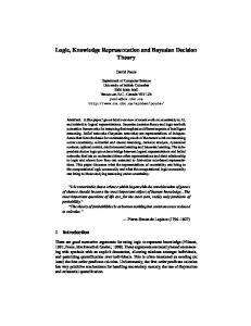
The Prior As a function: 1 −(p−(0.95α+0.05))2 e c where c is a normalizing constant. f (α, p) is then just a squared Gaussian with mean 0.95α + 0.05. This is the rate of enclisis found in the Tycho Brahe corpus. f (α, p) =

1.0 0.8 density 0.6 1.0 0.8 0.6

1.0 0.8

0.4

0.6

p (enclisis) 0.2

0.4 0.2 alpha (Prop. EP)

0.00.0

Figure: The prior density: f (α, p)

The Utility Function I

The learner wants to acquire the same grammar as the rest of its community.

I

The learner wants to be able to play both roles of speaker and hearer successfully.

I

A speaker of ClP will be able to understand both EP and ClP speakers without any penalty. However, a speaker of EP will have difficulty understanding ClP speakers. Conversely, EP speakers will be able to converse without penalty but not vice-versa.

I

Assume the individual plays speaker/hearer half the time.  U(a, α, p) =

if a = 0 (GClP ), − 21 α − 12 (1 − α) if a = 1 (GEP ).

This is also where we should be encoding pronounciation difficulty!

Utility Maximization The learner does not actually know what α and p are. They need to infer it from frequencies k and N. Instead of trying to pin this down (or stipulate it) expected utility maximization hedges its bets. So, Z E[U(a, α, p)|SN ] = U(a, α, p)dP(α, p|SN ). [0,1]2

To find out whether the parameter should be set ‘off’ (and simplified), we calculate: E[U(0, α, p)|SN ] > E[U(1, α, p)|SN ]. Z (2α − 1)P(SN |α, p)f (α, p)d(α, p) < 0 [0,1]2

If this last statement is true, the learner should choose GClP .

Estimating Production Rates I

Assume that production probabilities are derivable from the frequencies observed in the acquisition process.

I

For a ClP speaker: P(a1 |x1 ) = (N − k)/N, P(a2 |x1 ) = k/N

I

For an EP speaker: P(a2 |x1 ) = 1.

I

Let α0 be the proportion of GEP speakers observed in generation 0. Then the probability of getting the enclitic version in the first round. q0 = Ppop (a2 |x1 , T = 0) = (1 − α0 )p0 + α0

Over and Over...

I

The proportion of speakers who will see k enclitic constructions in N Bernoulli trials is:   N c q (1 − qt )N−k k t where qt is probability of seeing an enclitic in generation t.

I

This proportion of speakers will then contribute enclitics with a rate of k/N to the next generation, t + 1.

0.6 0.4 0.0

0.2

Rate of enclisis

0.8

1.0

Initial GClP rate of enclisis between 60-70%

0

50

100

150

200

250

300

Iteration no.

Figure: Rate of enclisis. N = 100, α0 = 0, and the initial rate of GClP enclisis, p, ranges from 0.6 to 0.7.

Change doesn’t take off from p = 0.05!

More interactions?

I

The stability of GClP is really assumed by the model via the prior.

I

Crucially, the simulation above still does not incorporate the effects of simultaneous change in other modules of language (e.g. phonology).

I

Production changes? We could define a new decision problem that estimates production probabilities.

Conclusion Take home points: I

This model articulates the general social learning model Niyogi (2006): learners learn from an (infinite) population.

I

The decision procedure was presented as a utility maximizing decision rule where the learner estimates population frequencies in order to maximize communicability.

I

Ideally we would look at a change in progress where we could do better estimation of the prior and utility functions.

Thanks! Especially to: Charles Yang, Andrew Clausen, and Ling 575/506-ers!

Simulation: 300 iterations

0.6 0.4 0.2 0.0

Proportion of EP

0.8

1.0

Figure: Transition diagram: Proportion of GEP speakers. Different curves represent different GClP enclisis rates (p): 0.05, 0.1, 0.2, 0.5, 0.8, and 1. n = 100 and α = 0.

0.0

0.2

0.4

0.6

Proportion of EP

0.8

1.0

Different input sizes

0.6 0.4 0.2 0.0

Rate of enclisis

0.8

1.0

Figure: Transition diagram: Overall rates of enclisis. Different curves represent different input sizes n: n = 10, 20, 50, 80, 100. α = 0

0.0

0.2

0.4

0.6

Rate of enclisis

0.8

1.0

0.6 0.4 0.0

0.2

Proportion of EP speakers

0.8

1.0

Initial GClP rate of enclisis between 60-70%

0

50

100

150

200

250

300

Iteration no.

Figure: Proportions of GEP speakers. n = 100, α0 = 0, and the initial rate of GClP enclisis, p, ranges from 0.6 to 0.7.

Portuguese BIL Example

I

If there is a 1-1 mapping between a meaning x and a type y then P(y |x, G ) = 1 − , if G admits x ( is an error term).

I

Let frequencies for input be: a1 = a, a2 = b, a3 = c.

I

Let, x1 , x3 be the meanings associate with a1 and a3 respectively.

I

We do not need to consider the contribution of obligatory proclisis to calculate the MLE (or MAP) grammar.

P(G |Yk , Xk ) ∝ P(Yk |Xk , G )P(G ) =

k Y

P(yi |xi , G )P(xi )

i=1 0

= P(a1 )a P(a2 )b P(a3 )c P(a1 |x1 , G )a P(a1 |x3 , G )a 0

00

0

00

P(a2 |x1 , G )b P(a2 |x3 , G )b

P(a3 |x1 , G )c P(a3 |x3 , G )c P(G ) Where a = a0 + a00 and similarly for the other frequency counts. Proclisis in affirmative sentences is simply given the error probability, , in GEP .

00

If we only care about finding MLE (or MAP) grammar, and taking probabilities from Nigoyi’s implementation of GBM, then we have the following.

P(GClP |Yk , Xk ) ∝ P(GClP )

(p − /2) ((1 − 2p − /2) (1 − p − ))a0 (1 − p − )b0 0

P(GEP |Yk , Xk ) ∝ P(GEP )(/2)a (1 − /2)b

0

I

The explicit connection between meaning and types allows us to reduce the parameter space needed to evaluate the two grammars in question.

I

We only need to parameterize the error term to do the the likelihood computation for GEP . In general, it will allow us to focus only on types that show variation.

I

The prior notwithstanding, this reduction in the parameter space is welcome in comparison with Nigoyi’s implementation.

I

However, this still suffers from over-parameterization the problems associated with MLE. P(a1 |x1 ) = p is still assumed to be an innate part of the grammar.

Briscoe, E. J. (2002). Grammatical acquisition and linguistic selection. In Briscoe, E. J., editor, Linguistic Evolution through Language Acquisition: Formal and Computational Models, chapter 9. Cambridge University Press. Briscoe, T. (2000). Grammatical Acquisition: Inductive Bias and Coevolution of Language and the Language Acquisition Device. Language, 76(2):245–296. Costa, J. and Duarte, I. (2002). Preverbal sbjects in null subject languages are not necessarily dislocated. Journal of Portuguese Linguistics, 2:159–176. Dowman, M., Kirby, S., and Griffiths, T. L. (2006). Innateness and culture in the evolution of language. In Proceedings of the 6th International Conference on the Evolution of Language, pages 83–90. Galves, A. and Galves, C. (1995). A case study of prosody driven language change: from classical to modern European Portuguese. Unpublished MS, University of Sao Paolo, Sao Paolo, Brasil.

Galves, C. (2003). Clitic-placement in the history of portuguese and the syntax-phonology interface. In Talk given at 27th Penn Linguistics Colloquium, University of Pennsylvania, USA. Galves, C., Britto, H., and Paix˜ao de Sousa, M. (2005a). The Change in Clitic Placement from Classical to Modern European Portuguese: Results from the Tycho Brahe Corpus. Journal of Portuguese Linguistics, pages 39–67. Galves, C., de Sousa, P., and Clara, M. (2005b). Clitic Placement and the Position of Subjects in the History of European Portuguese. In Geerts, T., Ginneken, V., Ivo, and Jacobs, H., editors, Romance Languages and Linguistic Theory 2003: Selected papers from ’Going Romance’ 2003, pages 97–113. John Benjamins, Amsterdam. Griffiths, T. and Kalish, M. (2005). A Bayesian view of language evolution by iterated learning. In Proceedings of the XXVII Annual Conference of the Cognitive Science Society. Kirby, S. (2001). Spontaneous evolution of linguistic structure: an iterated learning model of the emergence of regularity and

irregularity. IEEE Transactions on Evolutionary Computation, 5(2):102–110. Kirby, S., Dowman, M., and Griffiths, T. (2007). Innateness and culture in the evolution of language. Proceedings of the National Academy of Sciences, 104(12):5241. Kirby, S. and Hurford, J. (2002). The emergence of linguistic structure: An overview of the iterated learning model. In Cangelosi, A. and Parisi, D., editors, Simulating the Evolution of Language, chapter 6, pages 121–148. Springer-Verlag. Matsen, F. A. and Nowak, M. A. (2004). Win-stay, lose-shift in language learning from peers. PNAS, 101(52):18053–18057. Mitchener, W. and Nowak, M. (2003). Competitive exclusion and coexistence of universal grammars. Bulletin of Mathematical Biology, 65(1):67–93. Niyogi, P. (2006). The computational nature of language learning and evolution, chapter 7. MIT Press. Niyogi, P. and Berwick, R. (1998). The Logical Problem of Language Change: A Case Study of European Portuguese. Syntax, 1(2):192–205.

Nowak, M., Plotkin, J., and Krakauer, D. (1999). The evolutionary language game. Journal of Theoretical Biology, 200(2):147–162. Yang, C. (2001). Internal and external forces in language change. Language Variation and Change, 12(03):231–250.