Bayesian Framework for Multidisciplinary

Submit to NASA LaRC Multidisciplinary Uncertainty Quantification Challenge

Bayesian Framework for Multidisciplinary Uncertainty Quantification and Optimization Chen Liang and Sankaran Mahadevan Vanderbilt University, Nashville, TN - 37235

This paper presents a comprehensive methodology that combines uncertainty quantification, propagation and robustness-based design optimization using a Bayesian framework. Two types of epistemic uncertainty regarding model inputs/parameters are emphasized: (1) uncertainty modeled as p-box, and (2) uncertainty modeled as interval data. A Bayesian approach is used to calibrate the uncertainty models, where the likelihood functions are constructed using limited experimental data. The calibrated (improved) models are validated by partially characterized data using an area metric. A global sensitivity analysis (GSA), which previously only considered aleatory uncertainty, is extended to identify the contribution of epistemic uncertainty using an auxiliary variable method. A decoupled robustness-based design optimization framework is developed for optimization under both aleatory and epistemic uncertainty. Gaussian Process (GP) surrogate modeling is employed to improve the computational efficiency. The proposed methodology is illustrated using the NASA Langley multidisciplinary uncertainty quantification challenge problem1.

I. Introduction This paper addresses the multidisciplinary uncertainty quantification challenge problem proposed by researchers at NASA Langley Research Center. The mathematical model describes the dynamics of the Generic Transport Mode (GTM) 1. The multidisciplinary system is composed of two levels of analyses: level 1 computes 𝒙 as functions of input parameters 𝒑, and level 2 evaluates the model output 𝒈 as a function of 𝒙 and design variables 𝒅. For a particular design point 𝒅∗ , the presence of uncertainty in 𝒑 results in the randomness in 𝒙, consequently the model output 𝒈 is stochastic. In this context, the challenge problem proposed five objectives: uncertainty characterization, sensitivity analysis, uncertainty propagation, extreme-case analysis and robust design. Section 2 addresses the first objective, which requires the analyst to reduce the epistemic uncertainty of 𝒑 given available experimental data. The reduced uncertainty model is then validated with a different set of experimental data using an area metric. Section 3 extends the method of global sensitivity analysis (GSA) to quantify the significance of epistemic uncertainty using an auxiliary variable approach. Section 4 estimates the ranges of selected statistics of variables that depend on 𝒑, and identifies the realizations of 𝒑 that yield the bounds of these ranges using an optimization approach. Section 5 adopts an un-nested framework for robustness design under uncertainty. Sources of uncertainty can be classified into two categories: (1) Aleatory uncertainty due to the inherent physical variability in all processes; this is irreducible. The variability may be represented by probability distributions, whose distribution type and parameters are estimated from the data. (2) Epistemic uncertainty, which arises from the lack of knowledge about model variables (model input and model parameters) as well as the modeling process itself (model form assumptions and solution approximations). The emphasis of the challenge problem is mainly on epistemic uncertainty; regarding model variables, epistemic uncertainty can occur in two ways: (i) a stochastic but poorly known quantity2 and (ii) a deterministic but poorly known quantity3. The quantification and propagation methods for aleatory uncertainty are well-established. In the past few years, there is an increasing emphasis on uncertainty propagation and design optimization considering both aleatory and epistemic uncertainty. The representation of epistemic uncertainty and its propagation through models are of major interest. In probabilistic analysis, epistemic uncertainty has been represented by p-boxes3, a family of distributions4 instead of a single distribution, or a non-parametric PDF5. Non-probabilistic techniques such as evidence theory6 and possibility theory7 have also been pursued. In this challenge problem, the probabilistic representation of epistemic uncertainty is composed of: (1) p-boxes, where the distribution type is known while the parameters of the distribution are only available as intervals; and (2) interval representation for a deterministic but unknown quantity. A Bayesian approach is commonly used to reduce the uncertainty from the input given observations of the output. To measure the performance of an uncertainty model requires model validation techniques. Model validation aims at comparing model predictions with observed experimental outcomes to assess the accuracy of a particular simulation model8. It is also argued that the metric should depend on the number of experimental replications of a measurement quantity, and should only measure the agreement between the computational results and the

1

experimental data9. Ling and Mahadevan investigated different validation methods including classical and Bayesian hypothesis testing, a reliability-based method and an area metric-based method, and develops new insights into quantitative methods for model validation10. The second thrust of the challenge problem is quantitative sensitivity analysis. The objectives of sensitivity analysis are usually in two directions: (1) determination of the dominant uncertainty sources to improve such that the output uncertainty can be reduced the most, and (2) identification of the uncertainty sources whose contributions are sufficiently trivial such that they can be assumed as a fixed constant. Sensitivity analysis regarding aleatory uncertainty has been well-studied, yet little research has been done with respect to the sensitivity to epistemic uncertainty. This paper adopts a variance decomposition-based global sensitivity analysis (GSA)11 under both aleatory and epistemic uncertainty by exploiting an auxiliary variable method12. The third objective is to propagate the aleatory/epistemic uncertainty through the two-leveled system and quantify the output uncertainty. Aleatory uncertainty can be modeled as a random variable with fixed probability distributions and distribution parameters; a variety of approaches such as Monte Carlo Methods, first-order reliability method (FORM), second-order reliability method (SORM), etc. can be used for the propagation of aleatory uncertainty13. Efficient alternatives, in the presence of aleatory uncertainty alone, have been investigated by many researchers. Gu et al.14 proposed worst case uncertainty propagation using derivative-based sensitivities. Kokkolaras et al.15 used the advanced mean value method for uncertainty propagation and reliability analysis. Liu et al. 16 extended the same method by using moment-matching and considering the first two moments. However, no sensitivity has been reported including epistemic uncertainty. In this research, the uncertainty propagation of both aleatory and epistemic uncertainty is considered under a Bayesian framework. An optimization method is proposed to directly estimate the ranges of the output uncertainty. The realizations of uncertainty models that result in the ranges can also identified using the proposed method. To improve computational efficiency, the high fidelity analysis model is replaced by a Gaussian Process surrogate model which is computationally cheap. The thrust of the final objective is robustness-based design under uncertainty. Optimization under uncertainty within engineering design has been pursued in two directions: (1) reliability-based design optimization (RBDO)17, where the focus is on achieving desired reliability levels for constraints, and (2) robustness-based design optimization (RDO)18, where a design that is insensitive to different uncertainty sources is desired. The components of robustnessbased design optimization are: (1) maintaining robustness in the objective function (objective robustness); (2) maintaining robustness in the constraints (feasibility robustness); (3) estimating mean and measure of variance of the performance function; and (4) multi-objective optimization19. This paper focuses on robustness-based design optimization under epistemic uncertainty. Only a few studies on robustness design optimization considering epistemic uncertainty have been reported in the literature. Youn et al.7 made use of a possibility-based method based on fuzzy theory. Zaman et al.19 developed a probabilistic format to represent epistemic uncertainty for the sake of uncertainty propagation19. This paper adopts the RDO framework developed by Zaman et al. to incorporate both aleatory and epistemic uncertainty. The contributions of this paper are as follows: 1) Provide a comprehensive methodology for epistemic uncertainty quantification, propagation and robustnessbased design optimization; 2) Develop an approach to quantify the contribution of epistemic uncertainty sources to system output uncertainty; 3) Incorporate uncertainty quantification within a decoupled framework to improve the efficiency of robustness design optimization; 4) Demonstrate the proposed methodology for the NASA LaRC UQ challenge problem1.

II.

Uncertainty Characterization using the Bayesian Approach

The outputs of level 1 analysis 𝒙𝟏 are composed of 5 variables. The first subproblem asks analyst to make use of the available experimental data of 𝒙𝟏 to reduce its input epistemic uncertainty: 𝒑 = [𝑝1 , 𝑝2 , 𝑝4 , 𝑝5 ]. Based on Bayes theorem, a Bayesian inference methodology is employed to account for all the epistemic uncertainty. Section 2.1 gives a brief overview of the Bayes theorem. Section 2.2 discusses the application of Bayes theorem in updating the distribution of the uncertain parameters. Section 2.3 presents the updated uncertainty models using different number of experimental data and validate the updated models using an area metric.

2

2.1 Bayesian Methodology A common usage of Bayes’ theorem is to infer the posterior distribution of unknown parameters given observation data (evidence). Mathematically, Bayes’ theorem describes the relationship between the probabilities of 𝐴 and 𝐵, and the conditional probabilities of 𝐴 given 𝐵 and 𝐵 given 𝐴:

𝑃(𝐴|𝐵) =

𝑃(𝐵|𝐴)𝑃(𝐴)

(1)

𝑃(𝐵)

In the context of Bayesian inference, given the observation data 𝐷, the posterior distribution of the dependent parameters 𝜃 can be estimated as

𝑓 ′′ (𝜃) =

𝐿(𝜃)𝑓 ′ (𝜃) ∫ 𝐿(𝜃)𝑓 ′ (𝜃)𝑑𝜃

(2)

where the likelihood function 𝐿(𝜃) is defined as 𝐿(𝜃) = 𝑃(𝐷|𝜃)

(3)

The integral in Eq. 2 is usually difficult to evaluate when the prior distribution 𝑓 ′ (𝜃) is continuous. Therefore, Eq. 2 is often written as 𝑓 ′′ (𝜃) ∝ 𝐿(𝜃)𝑓′(𝜃)

(4)

The posterior distribution is evaluated using techniques such Markov Chain Monte Carlo (MCMC) sampling. Several MCMC algorithms based on acceptance – rejection sampling are used in practice (e.g., Metropolis-Hastings20, Gibbs21, etc.). 2.2 Model Characterization The Bayesian inference method is usually pursued to solve three types of problems: (1) update distribution parameters of an observed variable, (2) update distribution parameters of input variables to a model, and (3) update distributions of coefficients in a model, which is also known as model calibration or Bayesian regression. The subproblem I is the second type here, where the distribution parameters of the input variables are given as intervals and need to be updated using the observed data. The epistemic inputs of the model are [𝑝1 , 𝑝2 , 𝑝4 , 𝑝5 ], and the output is 𝑥1 . For epistemic uncertainty modeled as p-box, the distribution parameters are given as intervals; therefore, uniform distributions is assumed as their prior distributions, of which the upper and lower bounds are denoted as 𝑢𝑏 and 𝑙𝑏. The treatment for a fixed but unknown quantity is similar: uniform distribution bounded by the given interval is assumed as prior. The distributions are updated using 25 and 50 experimental data; the posterior distributions of the parameters are given in Table 1, the PDFs are shown in Figure 1. In Table 1, the first row (i.e., number of data points=0) gives the prior distributions. Table 1. Updated uncertainty models Number of Calibrating Data 0 25 50

𝑙𝑏 𝑢𝑏 𝜇 var 𝜇 var

𝑬[𝒑𝟏 ]

𝑽𝒂𝒓[𝒑𝟏 ]

𝒑𝟐

𝑬[𝒑𝟒 ]

𝑽𝒂𝒓[𝒑𝟒 ]

𝑬[𝒑𝟓 ]

𝑽𝒂𝒓[𝒑𝟓 ]

𝝆

0.600 0.800 0.679 0.002 0.742 0.001

0.020 0.040 0.030 3.29E-05 0.030 3.05E-05

0.000 1.000 0.441 0.109 0.506 0.082

-5.000 5.000 1.165 0.218 -2.037 0.787

0.0025 2.000 2.313 1.293 1.177 1.238

-5.000 5.000 -0.126 0.639 2.575 5.841

0.0025 2.000 1.366 0.579 1.334 0.229

-1.000 1.000 -0.480 0.162 0.023 0.178

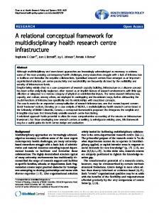
To test the performance of the improved uncertainty models in predicting the observational data, a model validation technique is required. Figure 2 shows the prior and posterior distribution of 𝒙𝟏 as well as the distribution of data of 𝒙𝟏 for calibration and validation. Note that the validation data are resulting from partially characterized experiments, where the inputs of the experiment are not measured or are reported as intervals. Consequently, they have more uncertainty than validation data from fully characterized experiments, where all inputs are measured and given as point value. An area metric is adopted as a measure the extent of agreement between model predictions and experimental data.

3

Figure 1. Prior and posterior distributions of uncertainty models

Figure 2. Prior and posterior distribution of 𝒙𝟏 as well as the distribution of calibration and validation data

2.3 Model Validation The area metric was proposed by Ferson et al.22. This metric provides a direct and quantitative yet computationally easy measure of the model prediction quality. As mentioned in the challenge problem, the experimental observation (𝑋𝐷 ) is random due to measurement error. In the presence of both aleatory and epistemic uncertainty, the model output (𝑋𝑀 ) is also stochastic. The area metric measures the difference between the cumulative distribution functions (CDF) of model output and the validation data, which is defined as +∞

𝑑(𝐹𝑋𝑚 − 𝑆𝑋𝐷 ) = ∫−∞ (𝐹𝑋𝑚 (𝑥) − 𝑆𝑋𝐷 (𝑥)) 𝑑𝑥

(5)

where 𝐹𝑋𝑚 is the CDF of model output and 𝑆𝑋𝐷 is the empirical CDF of the validation data. To account for the effect of the number of observations on the fidelity of the resulting uncertainty models, the epistemic uncertainty models are updated using 10 and 25 experimental data respectively. After that, random samples of 𝒑 are generated from the posterior distributions to calculate 𝑋1 . Then each sample of 𝑋1 is used to take difference with all 25 validation points 𝑋1𝑣𝑎𝑙 . The area metric is then computed using Eq. 5 and the results are given in Table 2: Table 2. Area metrics for models Model Area Metric Prior 0.0219 Updated by 10 Samples 0.0439 Updated by 25 Samples 0.0348

4

It can be observed that the prior distribution gives the smallest metric, which indicates that it agrees well with the distribution of validation data. Also, the majority of the calibration data concentrate between 0.3 and 0.4, whereas the validation data mainly locate between 0.2 and 0.3. This inconsistency between the calibration and validation data leads to an incremental area metric of the posterior distribution after updated by 10 samples, and the difference is mitigated by adding more calibration data.

III.

Sensitivity Analysis for Epistemic Uncertainty

3.1 Global Sensitivity Analysis The second objective requires a sensitivity analysis to identify the significant contributors to the system output uncertainty. Possible benefits for sensitivity analysis include: (1) reduction of number of uncertainty sources considered in the analysis; (2) indication for resource allocation such as expenses and computational cost; and (3) guidance for model refinement; benefits (1) and (3) are the thrusts of this objective. A global sensitivity analysis approach11 is used to study the contributions of multiple types of uncertainty to the overall prediction uncertainty. Note that this approach is based only on second-moment calculations, and calculates the effect of the variance of an input quantity on the variance of the output quantity. Consider a model given by 𝑌 = 𝐺(𝑋1 , 𝑋2 … 𝑋𝑛 )

(6)

where 𝑋𝑖 and 𝑌 are input-output pairs of a generic model. The first-order sensitivity indices are given by:

𝑆𝑖1 =

𝑉𝑋𝑖 (𝐸𝑋~𝑖 (𝑌|𝑋𝑖 )) 𝑉(𝑌)

(7)

where the notation 𝐸𝑋~𝑖 (𝑌|𝑋𝑖 ) denotes the expectation of output 𝑌 given a particular value of 𝑋𝑖 and considering the random variations of all other variables except for 𝑋𝑖 (denoted by 𝑋~𝑖 ). The symbol 𝑉𝑋𝑖 represents the variance of the aforementioned expectation over multiple samples of 𝑋𝑖 . The first-order sensitivity index indicates the contribution of uncertainty due to a particular individual variable, regardless of its interactions with other variables. The evaluation of Eq. 7 can be accomplished by either a double-loop or single-loop Monte Carlo Method. The sum of first-order indices of all variables is always less than or equal to unity. In the challenge problem, uncertainty models represented by a p-box consist of multiple parameters as random variables (e.g., mean and variance of 𝒑𝟏 are both random variables). Simply adding the indices together will underestimate the actual effect of these variables. Therefore, a higher-order sensitivity index is adopted to account for the combined effect of random variables describing the same uncertainty model. Assuming that 𝑋𝑖 and 𝑋𝑗 are random variables that describe an uncertainty model, their combined effect can be represented by a second-order index estimated as 𝑉𝑋𝑖 𝑋𝑗 (𝐸𝑋~𝑖,~𝑗 (𝑌 |𝑋𝑖 , 𝑋𝑗 )) 𝑉(𝑌)

= 𝑆𝑥1𝑖 + 𝑆𝑥1𝑗 + 𝑆𝑥𝑖𝑥𝑗

(8)

Note that usually the higher-order sensitivity indices need to be evaluated for all the combinations of the variables. In the challenge problem, prior knowledge of the input-output relations among the variables is given, therefore only the combined effect of the variables that describe the same uncertainty model is quantified. 3.2 Auxiliary Variable Method Given particular values of the parameters, the output of an uncertainty model is a probability distribution. This makes it difficult to evaluate Eq. 8, since the expectation can only be calculated when the output 𝑌 is a deterministic quantity for a given value of 𝑋𝑖 and 𝑋𝑗 . An auxiliary variable method defined by Sankararaman and Mahadevan23 is used below to overcome this challenge. For the sake of illustration, consider a normal random variable 𝑋 with uncertain parameters: 𝜇𝑋 and 𝜎𝑋 . Assuming that 𝜇𝑋 ~𝑁(𝜇𝜇 , 𝜎𝜇 ) and 𝜎𝑋 ~ Beta(𝛼𝜎 , 𝛽𝜎 ), where 𝜇𝜇 , 𝜎𝜇 , 𝛼𝜎 and 𝛽𝜎 are based on sources such as experts opinion. Given a realization of 𝜇𝑋 and 𝜎𝑋 , 𝑋 is a distribution. Let 𝑃 denote the auxiliary variable, defined by the probability integral transform24:

5

𝑥

𝑃 = ∫ 𝑓𝑋 (𝑋|𝜇𝑋 , 𝜎𝑋 )𝑑𝑋

(9)

−∞

where 𝑥 is a generic realization of 𝑋 and 𝑃 ∈ [0,1] is the CDF value. For a realization of 𝜇𝑋 and 𝜎𝑋 , the well-known inverse CDF method of Monte Carlo simulation taken over a realization of 𝑃 from a uniform distribution gives a fixed value of 𝒙. Therefore, 𝒙 can be written as −1 𝒙 = 𝐹𝑋|𝜇 (𝑝) 𝑋 ,𝜎𝑋

(10)

By introducing the auxiliary variable 𝑃 , we get a unique value of 𝑋 for a given value of 𝜇𝑋 and 𝜎𝑋 . The probability integral transform helps to define the auxiliary variable 𝑃, and will be used to include the stochastic model output for sensitivity analysis. In this case, if a discrete variable 𝐷 represents the distribution type, and Θ represents the vector of distribution parameters, then a unique value of 𝑥 can be obtained for a realization of 𝐷, 𝜃 and 𝑃 as

𝒙 = 𝐻(𝑝, 𝑑, 𝜃)

(11)

−1 where 𝐻(𝑝, 𝑑, 𝜃) = 𝐹𝑑,𝜃 (𝑝). To identify the contribution of epistemic uncertainty, this auxiliary variable method is used to delineate the uncertainty of a variable into two components: (1) The parameter distribution uncertainty (epistemic) represented by 𝐷, Θ and (2) variability (aleatory) represented by the auxiliary variable 𝑃.

3.3 Computational Issue As mentioned before, the mathematical model contains two levels of analyses. The computation from 𝒑 to 𝒙 is relatively cheap, while calculation from 𝒙 (and 𝒅 ) to 𝒈 is computationally intensive to be used repeatedly in calculating the model output in GSA. Therefore, a Gaussian Process (GP) surrogate modeling technique is employed to replace the high fidelity model and improve the computational efficiency. The GP modeling technique has been used in a wide range of applications requiring data regression and model calibration. A GP regression or interpolation models the underlying covariance within the data instead of the actual function form. With a set of training points 𝑿𝑻 = {𝑥1 , 𝑥2 , … 𝑥𝑛 } and the corresponding model outputs: 𝒚 𝑇 = {𝑦1 , 𝑦2 , … 𝑦𝑛 }, the GP model estimates the mean and variance at the prediction points 𝑿𝑷 : (12) 𝑚 = 𝐾𝑃𝑇 (𝐾𝑇𝑇 + 𝜎𝑛2 𝐼)−1 𝑦𝑇 𝑆 = 𝐾𝑃𝑃 − 𝐾𝑃𝑇 (𝐾𝑇𝑇 + 𝜎𝑛2 𝐼)−1 𝐾𝑇𝑃

(13)

where 𝑲 𝑇𝑇 = [𝑘(𝑥𝑖 , 𝑥𝑗 )]𝑖,𝑗 is the 𝑡 × 𝑡 matrix of the covariance between 𝑿 𝑇 ; 𝑲𝑃𝑃 is the 𝑝 × 𝑝 matrix of the

covariances between 𝑿𝑃 ; 𝑲𝑃𝑇 and 𝑲 𝑇𝑃 are the 𝑝 × 𝑡 matrix of covariance matrix between 𝑿𝑃 and 𝑿 𝑇 and its transpose matrix. Function evaluations with GP surrogate model are inexpensive; therefore it is can be used to replace expensive high-fidelity computational model in activities such as uncertainty propagation and optimization under uncertainty25. In this section, at a fixed design value, GP models are trained using 𝒙 and 𝒈 values. A Latin hypercube sampling is adopted to generate the training point inputs. 3.4 Results and Discussions In the level 1 mathematical model, there are 17 model inputs 𝒑 and 5 outputs 𝒙. The uncertainty of 𝑥5 entirely depends on its only input 𝑝21 . Given a particular value of distribution parameter, the auxiliary variable approach helps to generate deterministic output hence ensures the GSA under epistemic uncertainty. Table 3 ranks the significance of the inputs to the 5 outputs respectively.

Rankings 1 2 3 4

Table 3. Sensitivity indices for 𝒙 𝒙𝟏 𝒙𝟐 𝒙𝟑 parameter % parameter % parameter % 99.03 50.23 97.91 𝒑𝟏 𝒑𝟔 𝒑𝟏𝟐 0.86 47.74 0.87 𝒑𝟓 𝒑𝟕 𝒑𝟏𝟒 0.09 2.00 0.19 𝒑𝟒 𝒑𝟖 𝒑𝟏𝟓 0.01 0.03 0.04 𝒑𝟐 𝒑𝟏𝟎 𝒑𝟏𝟑

6

𝒙𝟒 parameter 𝒑𝟏𝟔 𝒑𝟏𝟖 𝒑𝟏𝟕 𝒑𝟐𝟎

% 64.65 20.39 14.39 0.50

The percentage in Table 3 is calculated based on Eq. 7 and Eq. 8. In the challenge problem, a fixed constant is wanted for parameters that has insignificant impact on 𝒙, and estimate the incurred error. As mentioned before, 𝑉𝑋𝑖 (𝐸𝑋~𝑖 (𝑌|𝑋𝑖 )) first calculates the expectation of output 𝑌 at a particular value of 𝑋𝑖 and considering the random variations of 𝑋~𝑖 , and then computes the variance of this expectation over multiple samples of 𝑋𝑖 . This variance may also represent the “error” incurred by fixing the parameters at different constant values. For each 𝒙, parameters which have sensitivity indices less than 1% are chosen to be fixed at their mean values, which are evaluated using Monte Carlo sampling. These values and the variance/incurred error is given in Table 4: Table 4. Fixed parameters and the incurred error based on 𝒙 𝒑𝟐

𝒑𝟒

𝒑𝟓

𝝆

𝒑𝟏𝟎

𝒑𝟏𝟑

𝒑𝟏𝟒

𝒑𝟏𝟓

𝒑𝟐𝟎

Fixed value

0.5

0

0

0

0.5

0.25

0.32

0.5

0.63

Incurred error

2.43E-06

1.58E-05

1.46E-04

1.87E-07

6.45E-07

1.89E-05

3.71E-04

8.31E-05

2.07E-05

The final system outputs 𝒈 is an eight-dimension vector, which is calculated solely based on 𝒙 (at a particular design point 𝒅∗ ). The quantities of interest are: (1) 𝐽1 , which is the expected value of the worst-case of 𝒈, and (2) 𝐽2 , which is the failure probability of the worst-case of 𝒈 given the uncertainty greater than 0. For a particular realization of 𝒑, 𝐽1 and 𝐽2 are deterministic quantities. Since 𝒑 are random variables, 𝐽1 and 𝐽2 are consequently stochastic. Table 5 filters and ranks the epistemic uncertainty models by their contribution to 𝐽2 : Table 5. Sensitivity indices for 𝑱𝟏 and 𝑱𝟐 𝑱𝟏

𝑱𝟐

Variance

%

Variance

%

𝒑𝟏

1.45E-02

98.17%

1.43E-01

81.21%

𝒑𝟐𝟏

1.70E-04

1.15%

2.38E-02

13.47%

𝒑𝟏𝟐

1.44E-05

0.10%

7.75E-03

4.39%

𝒑𝟏𝟔

5.31E-06

0.04%

4.34E-04

0.25%

𝒑𝟓

8.36E-07

0.01%

3.40E-04

0.19%

𝒑𝟕

4.51E-05

0.30%

2.66E-04

0.15%

𝒑𝟏𝟕

5.86E-06

0.04%

1.74E-04

0.10%

𝒑𝟔

9.05E-06

0.06%

1.52E-04

0.09%

𝒑𝟒

1.51E-05

0.10%

9.46E-05

0.05%

𝒑𝟏𝟖

4.95E-07

0.00%

8.54E-05

0.05%

𝒑𝟏𝟒

3.22E-08

0.00%

4.01E-05

0.02%

𝒑𝟖

6.92E-07

0.00%

1.96E-05

0.01%

𝒑𝟏𝟎

1.40E-07

0.00%

7.84E-06

0.00%

𝒑𝟏𝟓

3.79E-08

0.00%

7.49E-06

0.00%

𝒑𝟐

4.66E-06

0.03%

4.67E-06

0.00%

𝒑𝟐𝟎

3.00E-08

0.00%

4.55E-06

0.00%

𝝆

3.43E-08

0.00%

2.32E-06

0.00%

𝒑𝟏𝟑

6.86E-09

0.00%

2.11E-06

0.00%

The challenge problem asks to determine 4 out of the 17 epistemic uncertainty models to be improved such that the ranges of 𝐽1 and 𝐽2 can be reduced the most. It can be observed from Table 5 that the effects of 𝒑𝟏 , 𝒑𝟏𝟐 and 𝒑𝟐𝟏 combined have 99.41% influence on the uncertainty of 𝐽1 and 99.07% of 𝐽2 . Refinement of these three variables would yield the most output uncertainty reduction. The choice of the fourth uncertainty model to be improved is arguable. Since the uncertainty of 𝐽1 will have a larger reduction than 𝐽2 once the three dominant models are refined, the choice of random variable based on the refinement of 𝐽2 is preferable. Considering 𝒑𝟓 and 𝒑𝟏𝟔 are competitive in that sense, 𝒑𝟏𝟔 is chosen because it has a larger impact on 𝐽1 also compared with 𝒑𝟓 . New uncertainty models of 𝒑𝟏 , 𝒑𝟏𝟐 , 𝒑𝟏𝟔 , 𝒑𝟐𝟏 with less variances are requested by the analyst and provided. These new uncertainty models and are referred as New Model, whereas the models updated by 50 experimental data in Table 1 are referred as Updated Model in the following sections. Since the chosen uncertainty models combined account for more than 99% of the

7

uncertainty for both 𝐽1 and 𝐽2 ; the rest of the parameters therefore can be assumed as constants without yielding significant error. Table 6 gives the assumed constants for the parameters and associated errors, which is equivalent to the variances in Table 5.

Fixed value Error ( 𝑱𝟏 ) Error ( 𝑱𝟐 )

𝒑𝟐

𝒑𝟒

0.5 4.66 E-06 4.67 E-06

Table 6. Fixed parameters and the incurred error based on 𝑱𝟏 and 𝑱𝟐

𝒑𝟓

𝒑𝟔

𝒑𝟕

𝒑𝟖

𝒑𝟏𝟎

𝒑𝟏𝟑

𝒑𝟏𝟒

𝒑𝟏𝟓

𝒑𝟏𝟕

𝒑𝟏𝟖

𝒑𝟐𝟎

𝝆𝟒𝟓

0

0

0.5

0.7

0.64

0.5

0.25

0.32

0.5

0.5

0.76

0.63

0

1.51 E-05 9.46 E-05

8.36 E-07 3.40 E-04

9.05 E-06 1.52 E-04

4.51 E-05 2.66 E-04

6.92 E-07 1.96 E-05

1.40 E-07 7.84 E-06

6.86 E-09 2.11 E-06

3.22 E-08 4.01 E-05

3.79 E-08 7.49 E-06

5.86 E-06 1.74 E-04

4.95 E-07 8.54 E-05

3.00 E-08 4.55 E-06

3.43 E-08 2.32 E-06

IV.

Uncertainty Propagation and Extreme Case Identification

The third and fourth objectives are interested in determining the ranges of 𝐽1 and 𝐽2 . The thrust of the third objective is to estimate the upper and lower limits for 𝐽1 and 𝐽2 , while the fourth objective requires estimating the realizations of the uncertainty models that yield such limits. Estimation of the limits can be related to an optimization problem, where the maximum and minimum value of 𝐽1 and 𝐽2 need to be evaluated, and the epistemic uncertainty models are used as design space (both the updated uncertainty models and the new models). The non-gradient based DIRect algorithm26 is employed to find a global optimum at first. The optimal solution is then used as the initial guess of a gradient-based active set algorithm for further search of the local optimum. The bounds of the outputs are given in Table 7, and the particular uncertainty models that result in the bounds are presented in Table 8. Table 7. Bounds of 𝑱𝟏 and 𝑱𝟐 𝑀𝑖𝑛 𝐽1

𝑀𝑎𝑥 𝐽1

Range

𝑀𝑖𝑛 𝐽2

𝑀𝑎𝑥 𝐽2

Range

Updated Model

0.011

0.233

0.222

0.070

0.856

0.786

New Model

0.031

0.23

0.199

0.496

0.746

0.250

Table 8. Uncertainty models that yield the bounds Updated Model

New Model

𝑀𝑖𝑛(𝐽1 )

𝑀𝑎𝑥(𝐽1 )

𝑀𝑖𝑛(𝐽2 )

𝑀𝑎𝑥(𝐽2 )

𝑀𝑖𝑛(𝐽1 )

𝑀𝑎𝑥(𝐽1 )

𝑀𝑖𝑛(𝐽2 )

𝑀𝑎𝑥(𝐽2 )

0.74

0.65

0.77

0.77

0.64

0.65

0.64

0.62

0.02

0.03

0.02

0.02

0.03

0.03

0.03

0.03

1.00

0.13

0.24

0.24

0.05

0.13

0.21

0.10

-1.22

-3.37

-0.61

-0.61

0.01

-3.37

-1.85

-1.97

3.96

1.00

2.02

2.02

3.95

1.00

1.97

3.96

4.97

3.46

2.00

2.00

-1.06

3.46

3.96

2.05

0.55

1.11

1.70

1.70

2.18

1.11

1.67

1.76

𝜌 𝑝6 𝑎𝑝7 𝑏𝑝7 𝑎𝑝8 𝑏𝑝8 𝑎𝑝10 𝑏𝑝10

0.96

0.48

0.01

0.01

-0.72

0.48

-0.01

0.04

0.00

0.25

0.87

0.87

0.00

0.25

0.83

0.08

0.98

1.62

2.18

2.18

0.98

1.62

3.11

3.54

1.08

0.73

0.85

0.85

1.08

0.73

0.70

0.62

7.45

12.43

10.82

10.82

7.99

12.43

10.75

10.69

4.29

6.97

5.97

5.97

4.29

6.97

6.06

5.99

1.53

3.76

3.04

3.04

1.52

3.76

3.01

3.09

4.75

3.95

3.17

3.17

4.75

3.95

4.21

1.78

𝑝12 𝑎𝑝13

0.00

0.75

0.54

0.54

1.00

0.75

0.98

1.00

0.41

0.49

0.58

0.58

0.42

0.49

0.47

0.47

𝜇𝑝1 𝑉𝑎𝑟𝑝1 𝑝2 𝜇𝑝4 𝑉𝑎𝑟𝑝4 𝜇𝑝5 𝑉𝑎𝑟𝑝5

8

𝑏𝑝13 𝑎𝑝14 𝑏𝑝14 𝑎𝑝15 𝑏𝑝15 𝑝16 𝑎𝑝17 𝑏𝑝17 𝑎𝑝18 𝑏𝑝18 𝑎𝑝20 𝑏𝑝20 𝑎𝑝21 𝑏𝑝21

2.07

1.27

1.54

1.54

1.00

1.27

1.53

1.56

0.93

1.86

1.56

1.56

2.17

1.86

1.14

1.97

2.41

1.35

1.71

1.71

1.01

1.35

2.17

1.04

7.10

6.68

6.28

6.28

5.44

6.68

6.82

5.48

5.29

5.70

6.13

6.13

5.29

5.70

6.11

6.05

1.00

0.75

0.50

0.50

0.75

0.75

0.80

0.76

1.06

1.51

1.37

1.37

1.06

1.51

1.56

1.07

1.00

1.11

1.23

1.23

1.00

1.11

1.22

1.36

1.00

1.82

3.73

3.73

4.27

1.82

2.65

2.76

0.55

0.89

0.93

0.93

0.55

0.89

0.93

0.79

7.53

9.02

10.33

10.33

7.53

9.02

10.49

8.57

4.71

7.29

6.46

6.46

4.71

7.29

6.44

4.71

0.42

0.57

0.52

0.52

0.87

0.57

0.89

0.98

29.62

13.23

25.92

25.92

19.00

13.23

22.33

19.70

It can be observed from Table 7 that the intervals between the bounds yielded by the new models are smaller than the updated models for both 𝐽1 and 𝐽2 . This is expected since the uncertainty introduced by the most significant factors decreases in the reduced model. Meanwhile, the reduction of 𝐽2 is greater than 𝐽1 due to the reason that 𝐽2 calculates the probability of failure, which is more sensitive to the changes of uncertainty than 𝐽1 which estimate the mean value of the output.

V.

Robustness-based Design Optimization

5.1 Un-nested optimization formulation The final objective asks the analyst to determine the values of the design parameters 𝒅 that minimize the maximum value of 𝐽1 and 𝐽2 individually, namely the optimal worst-case probabilistic performance under uncertainty. This formulation of the problem emphasizes the feasibility robustness of the system, and requires a nested optimization framework shown in Eq. 14. The outer loop minimizes worst case which is computed by the inner loop. 𝑚𝑖𝑛 (𝑚𝑎𝑥 𝐽𝒊 (𝒅, 𝒙)) 𝒅

𝒙

𝑠. 𝑡. 𝒅𝑳𝑩 ≤ 𝒅 ≤ 𝒅𝑼𝑩

(14)

𝒙 = 𝒙(𝒑) 𝒑 ~ 𝑫𝒊𝒔𝒕(𝜽) 𝜽𝑳𝑩 ≤ 𝜽 ≤ 𝜽𝑼𝑩 𝒊 = 𝟏 ,𝟐 In each iteration, the outer loop generates a design value of 𝒅, and the inner loop maximize 𝐽1 /𝐽2 conditioned on this design point. In the presence of uncertainty in the design/non-design variables, the nested approach repeats the inner loop design optimization for every iteration of the outer loop. This method is computationally expensive yet does not ensure convergence. A decoupled approach was previously proposed by Zaman19 to un-nest the design optimization from the epistemic uncertainty analysis and thereby alleviate the computational effort. The decoupled un-nested approach is formulated as in Eqs. 15 and 16: 𝒅∗ = argmin 𝐽𝒊 (𝒅, 𝒙(𝒑(𝜽∗ ))) 𝒅

𝑠. 𝑡. 𝒅𝑳𝑩 ≤ 𝒅 ≤ 𝒅𝑼𝑩

(15)

𝜽∗ = argmin 𝐽𝒊 (𝒅∗ , 𝒙(𝒑(𝜽))) 𝜽

𝑠. 𝑡.

𝜽𝑳𝑩 ≤ 𝜽 ≤ 𝜽𝑼𝑩 𝒊 = 𝟏 ,𝟐

9

(16)

where 𝒅∗ are fixed quantities in the optimization in Eq. 15 and 𝜽∗ are fixed quantities in the optimization in Eq. 16. The optimization problems in Eq. 15 and Eq. 16 are solved iteratively until 𝐽1 (𝐽2 ) converges. Note that only the parameters of epistemic uncertainty are involved in this optimization framework. For parameters with aleatory uncertainty, their values are randomly sampled from their distribution each time when they are used. Recall that 𝐽1 and 𝐽2 are statistical measures of 𝒈, which are expensive to evaluate. The aforementioned GP models used in sensitivity analysis describe the functional dependence between 𝒙 and 𝒈 for a fixed 𝒅 value. In the optimization problem, however, 𝒈 is a function of both 𝒙 and 𝒅. Therefore, new GP models needs to be calibrated as functions of both 𝒙 and 𝒅, and used in the optimization framework. 5.3 Results and Discussions The GP surrogate models are trained using 500 samples of 𝐷, 𝑋 and 𝐺 for the costly level-2 analysis. The optimal values of 𝒅 that minimize the largest value of 𝐽1 given by the method using GP models are 𝒅𝐽1 = [0.02, -0.17, -0.10, 1.53, 0.82, -0.14, -0.10, -0.48, -0.64, 0.24, 0.01, -0.14, 1.59, -0.05]; and the optimal values of 𝒅 that minimize the largest value of 𝐽2 are 𝒅𝐽2 = [ 0.02,-0.31,-0.13,-2.26,0.80,-0.16,-0.09,-0.31,-0.62,0.40,0.01,-0.19,1.11,-0.04]. Given these values of 𝒅, the ranges of 𝐽1 and 𝐽2 are recalculated using the methods for subproblem 3 and 4. According to the results given in Table 9, all boundary values of 𝐽1 and 𝐽2 are lower at the new design value than at the initial point. The range between the maximum and minimum value of 𝐽1 drops from 0.199 to 0.117 (41.2%), whereas the range of 𝐽2 decreases from 0.25 to 0.187 (25.2%). A more robust solution can be obtained by maximizing the minimum value of 𝐽1 and 𝐽2 . Table 9. Ranges of 𝑱𝟏 and 𝑱𝟐 at the new design point Min

Max

Range

𝑱𝟏

0.012

0.129

0.117

𝑱𝟐

0.267

0.456

0.189

The GSA is applied again only at the design points 𝒅𝐽1 and 𝒅𝐽2 . New GP models need to be trained with 𝑿 as the only inputs and the output 𝒈 estimated at 𝒅𝐽1 and 𝒅𝐽2 respectively. The new rankings are given in Table 10. Three out of the four chosen parameters in Section 3.4, i.e., 𝑝12 , 𝑝16 and 𝑝21 , drop to lower rankings, while uncertainty of 𝑝1 still has dominant effects on the output uncertainty for both 𝐽1 and 𝐽2 . It has been concluded according to Table 9 that although the maximum and minimum value of 𝐽1 and 𝐽2 are reduced, the ranges do not have significant changes. Also, in Table 10, the variances (particularly the variances of 𝑝1 ) appear to be similar to the variances in Table 5. These are expected because the most significant factor to the output uncertainty is the aleatory uncertainty of 𝒑𝟏 , which is irreducible. Therefore, even though the epistemic uncertainty from 𝒑𝟏 is reduced, the aleatory uncertainty remains dominant at different design. Table 10. Sensitivity indices for 𝑱𝟏 and 𝑱𝟐 at the new design point 𝑱𝟏

𝑱𝟐

Variance

%

𝒑𝟏

5.79E-03

95.89%

Variance

%

𝒑𝟏

2.15E-01

99.24%

𝒑𝟐

2.00E-04

3.31%

𝒑𝟏𝟒

7.19E-04

0.33%

𝒑𝟏𝟒

1.12E-05

0.19%

𝒑𝟒

6.83E-04

0.32%

𝒑𝟒

1.04E-05

0.17%

𝒑𝟐

1.04E-04

0.05%

𝒑𝟏𝟖

9.39E-06

0.16%

𝒑𝟏𝟓

6.83E-05

0.03%

𝒑𝟏𝟕

6.63E-06

0.11%

𝒑𝟐𝟏

1.87E-05

0.01%

𝒑𝟐𝟏

3.69E-06

0.06%

𝒑𝟏𝟏

1.46E-05

0.01%

𝒑𝟔

2.91E-06

0.05%

𝒑𝟏𝟕

1.37E-05

0.01%

𝒑𝟕

2.29E-06

0.04%

𝒑𝟏𝟑

1.37E-05

0.01%

𝒑𝟏𝟏

5.09E-07

0.01%

𝒑𝟓

5.57E-06

0.00%

𝒑𝟖

5.08E-07

0.01%

𝒑𝟏𝟐

4.09E-06

0.00%

𝒑𝟏𝟓

4.12E-07

0.01%

𝒑𝟏𝟖

3.32E-06

0.00%

10

𝒑𝟗

1.36E-07

0.00%

𝒑𝟕

2.36E-06

0.00%

𝒑𝟏𝟑

1.28E-07

0.00%

𝒑𝟏𝟔

1.60E-06

0.00%

𝒑𝟓

9.30E-08

0.00%

𝒑𝟔

1.33E-06

0.00%

𝒑𝟏𝟔

4.31E-08

0.00%

𝒑𝟐𝟎

7.04E-07

0.00%

𝒑𝟑

3.78E-08

0.00%

𝝆𝟒𝟓

5.52E-07

0.00%

𝒑𝟐𝟎

3.48E-08

0.00%

𝒑𝟗

2.50E-07

0.00%

𝒑𝟏𝟐

1.25E-08

0.00%

𝒑𝟖

1.27E-07

0.00%

𝝆

9.02E-09

0.00%

𝒑𝟏𝟎

1.87E-08

0.00%

𝒑𝟏𝟎

5.79E-09

0.00%

𝒑𝟑

3.21E-29

0.00%

𝒑𝟏𝟗

4.38E-09

0.00%

𝒑𝟏𝟗

3.21E-29

0.00%

VI.

Conclusions

This paper proposes a methodology to include uncertainty characterization, sensitivity analysis, uncertainty propagation and robustness design optimization using a Bayesian approach. The NASA Langley multidisciplinary challenge problem is adopted to illustrate the proposed methodology. Emphasizing on epistemic uncertainty, a Bayesian inference technique is employed to improve the epistemic uncertainty models given experimental data. A reliability metric is used to measure the improvement of the model prediction as the input uncertainty being reduced. Global sensitivity analysis, which previously was only used in the context of aleatory uncertainty, is extended to estimate the sensitivity for epistemic uncertainty using the auxiliary variable method. The contribution of an uncertainty model due to both aleatory and epistemic components is quantified using a higher-order sensitivity index. A GP surrogate modeling technique is used for further computational efficiency. By identifying and reducing the most important uncertain factor, the output uncertainty is reduced significantly. Finally, a robustness-based design optimization framework is proposed under epistemic uncertainty. An un-nested optimization formulation is adopted to avoid intensive computational effort and have a better control over the convergence. It is concluded that the conservative worst-case optimization formulation may still lead to designs that may violate the constraints. Future work is required to include the observational error from the experimental data and the surrogate model error introduced by using GP models in a constrained robustness-based design optimization framework.

Acknowledgements Support from NASA Langley Research Center is acknowledged. Discussion on the auxiliary variable approach with Dr. Shankar Sankararaman and Dr. You Ling are deeply appreciated.

References 1.

Crespo, L. G., Kenny, S. P. & Giesy, D. P. The NASA Langley Multidisciplinary Uncertainty Quantification Challenge. 1–9 (2012).

2.

Helton, J. C., Johnson, J. D. & Oberkampf, W. L. An exploration of alternative approaches to the representation of uncertainty in model predictions. Reliab. Eng. Syst. Saf. 85, 39–71 (2004).

3.

Ferson, S., Kreinovich, V., Hajagos, J., Oberkampf, W. & Ginzburg, L. Experimental Uncertainty Estimation and Statistics for Data Having Interval Uncertainty. Sandia National Laboratories (2007).

4.

Zaman, K., Rangavajhala, S., McDonald, M. P. & Mahadevan, S. A probabilistic approach for representation of interval uncertainty. Reliab. Eng. Syst. Saf. 96, 117–130 (2011).

11

5.

Sankararaman, S. & Mahadevan, S. Likelihood-based representation of epistemic uncertainty due to sparse point data and/or interval data. Reliab. Eng. Syst. Saf. 96, 814–824 (2011).

6.

Agarwal, H., Renaud, J. E., Preston, E. L. & Padmanabhan, D. Uncertainty quantification using evidence theory in multidisciplinary design optimization. Reliab. Eng. Syst. Saf. 85, 281–294 (2004).

7.

Du, L., Choi, K. K., Youn, B. D. & Gorsich, D. Possibility-Based Design Optimization Method for Design Problems With Both Statistical and Fuzzy Input Data. J. Mech. Des. 128, 928 (2006).

8.

Rebba, R., Mahadevan, S. & Huang, S. Validation and error estimation of computational models. Reliab. Eng. Syst. Saf. 91, 1390–1397 (2006).

9.

Oberkampf, W. L. & Barone, M. F. Measures of agreement between computation and experiment: Validation metrics. J. Comput. Phys. 217, 5–36 (2006).

10.

Ling, Y. & Mahadevan, S. Quantitative model validation techniques: New insights. Reliab. Eng. Syst. Saf. 111, 217–231 (2013).

11.

Sensitivity, G. & The, A. Global Sensitivity Analysis: The Primer. Wiley-Interscience (2008)

12.

Sankararaman, S., Uncertainty Quantification and Integration in Engineering Systems. (Doctoral dissertation, 2012).

13.

Haldar, A. & Mahadevan, S. Probability, reliability, and statistical methods in engineering design. (John Wiley, 2000).

14.

Gu, X., Renaud, J. E., Batill, S. M., Brach, R. M. & Budhiraja, a. S. Worst case propagated uncertainty of multidisciplinary systems in robust design optimization. Struct. Multidiscip. Optim. 20, 190–213 (2000).

15.

Kokkolaras, M., Mourelatos, Z. P. & Papalambros, P. Y. Design Optimization of Hierarchically Decomposed Multilevel Systems Under Uncertainty. J. Mech. Des. 128, 503 (2006).

16.

Liu, H., Chen, W., Kokkolaras, M., Papalambros, P. Y. & Kim, H. M. Probabilistic Analytical Target Cascading: A Moment Matching Formulation for Multilevel Optimization Under Uncertainty. J. Mech. Des. 128, 991 (2006).

17.

Valdebenito, M. a. & Schuëller, G. I. A survey on approaches for reliability-based optimization. Struct. Multidiscip. Optim. 42, 645–663 (2010).

18.

Du, X. & Chen, W. Towards a Better Understanding of Modeling Feasibility Robustness in Engineering. Journal of Mechanical Design. 122, 385–394 (2013).

19.

Zaman, K., McDonald, M., Mahadevan, S. & Green, L. Robustness-based design optimization under data uncertainty. Struct. Multidiscip. Optim. Press (2011).

20.

Chib, S., & Greenberg, E. Understanding the metropolis-hastings algorithm. The American Statistician, 49(4), 327-335. (1995).

21.

Casella, G., & George, E. I. Explaining the Gibbs sampler. The American Statistician, 46(3), 167174. (1992).

22.

Ferson, S., Oberkampf, W. L. and Ginzburg, L. Model validation and predictive capability for the thermal challenge problem. Comput. Methods Appl. Mech. Eng. 197, 2408–2430. (2008).

23.

Sankararaman, S. & Mahadevan, S. Separating the contributions of variability and parameter uncertainty in probability distributions. Reliab. Eng. Syst. Saf. 112, 187–199 (2012).

24.

Probability, T. et al. The Probability Integral Ttransformation for Testing Goodness of Fit and Combining Independent Tests of Significance. 30, 134–148 (1938). 12

25.

Rangavajhala, S., Liang, C., Mahadevan, S. Design Optimization Under Aleatory and Epistemic Uncertainties. Proc. 14TH AIAA/ISSMO Multidiscip. Anal. Optim. Conf. (2012).

26.

Bjorkman, M. & Holmstrom, K. Global Optimization Using the DIRECT Algorithm in Matlab, (1999).

13