Nov 22, 2000 - large-scale warping, varying row/column-spacing as well as non-rigid random fluctuations ... purpose of the arc prior is to model varying row- and column- spacing ...... A/S, http://www.viavision.dk/filer/ispot.html, 1998. [27] K.L. ...
Bayesian Grid Matching Karsten Hartelius Jens Michael Carstensen Institute of Mathematical Modelling Technical University of Denmark November 22, 2000 Abstract In this article we present a method for locating distorted grid-structures in images. The method is based on the theories of template matching and Bayesian image-restoration. The grid is modeled as a deformable template. Prior knowledge of the grid is described through a Markov Random Field (MRF) model which represent the spatial coordinates of the grid-nodes. Knowledge of how grid-nodes are depicted in the observed image is described through the observation model. The prior consists of a node prior and an arc prior, both modeled as Gaussian MRFs. The node prior models variations in the positions of gridnodes and the arc prior models variations in row- and column-spacing across the grid. Grid matching is done by placing an initial rough grid over the image and applying an ensemble annealing scheme to maximize the posterior distribution of the grid. The method can be applied to noisy images with missing grid-nodes and grid-node artifacts and the method accommodates a wide range of grid-distortions including: large-scale warping, varying row/column-spacing as well as non-rigid random fluctuations of the grid-nodes. The methodology is demonstrated in three case-studies concerning localization of 1) spots in 2D calibration sheets, 2) knit-units in textile-samples and 3) DNA-signals in hybridization filters.
1 Introduction The problem of locating grid-structures in images occurs frequently in image analysis applications, especially in the fields of graph-matching, pattern recognition, image warping, flow estimation and motion analysis. Here we are concerned with the problem of locating irregular grid-structures in images deviating from a fixed template shape. Objects with unique template shapes can often be found using rather simple image analysis methods. However nowadays many image analysis applications deals with objects and patterns that are natural and do not have single unique shapes. A fundamental problem within the field of grid-matching is to match a template-graph to a set of candidate points in an observed image, hereunder finding a geometric transformation for the point-mappings. There exist many approaches to this problem - the majority using graph-search algorithms, e.g. dynamic programming and maximum clique algorithms ([1],[2],[3]). The geometric transformation is normally obtained through parameterized transformations or by placing relations/constraints between neighboring points.
Here we regard a different scenario where a graph is matched to the observed image without using a set of candidate points. We handle the observed image in a probabilistic manner and determine the geometric transformation and the corresponding matching points jointly. We present a grid-matching methodology based on the theory of deformable templates and Bayesian restoration which is highly useful for finding distorted grid-structures. The methodology accommodates global deviations of the grid-structure including rotation and warping and local deviations such as non-rigid discontinuities and fluctuations of grid-nodes. The methodology also accepts that parts of the grid is hidden in the image due to noise or occlusion. The grid is defined as a deformable template which is allowed to deviate from regularity through a Markov random field deformation mechanism. Gridmatching is done through a simulated annealing scheme which performs an iterative deformation to match the grid to grid-node positions in the image. Fig. 1 show the principle of a deformable grid-template. [4] uses a Markov random field to describe the deformation of nodes in a two-dimensional grid. Here we describe grid-node interactions in a Gaussian framework which is more general. We present a graph node prior that can be used to model deformations of general graph-structures without limitations on dimensionality. For two-dimensional rectangular graphs we present a grid-prior consisting of both a node prior and an arc prior. The purpose of the arc prior is to model varying row- and columnspacing across the grid. Bayesian image analysis is highly suitable for modeling visual phenomena which are stochastic in nature ([5], [6], [7], [8], [9]) and has shown to provide powerful solutions within the fields of reconstruction, segmentation, classification and shape-analysis. [10] applies Bayesian restoration to the problem of matching warped images. Within graphmatching and object recognition the Bayesian framework has become more widespread. [11] describes a graph-matching methodology where an EM-algorithm is used to jointly perform point-matching and estimation of parameterized pointtransformations under the assumption that measurement errors are Gaussian distributed. The method is suitable for applications involving perspective transformations and is applied to the problem of aerial image registration. [12] describes a matching problem involving a collection of object primitives extracted from an image to be matched with a similar collection representing a template. The primitives are regarded as nodes in
a graph and binary relations between pairs of nodes constitute arcs in the graph. The binary relations include relative distanceand angle-metrics. It is assumed that the binary relation errors are Gaussian of nature and a probabilistic relaxation algorithm is used to fit the primitives to the template-collections. The method is applied to the task of recognizing aerial road network images based on road network models. [13] presents a method for matching pictorial structures in images. Pictorial structures are composed of picture-parts arranged in treeshaped graphs. Binary relations such as: angle, scale and translation are placed between neighboring parts and the best match is found by energy-minimization. An efficient dynamic programming algorithm is used to find an informal MAP estimate. The scheme is suitable for generic image recognition and is applied to the problem of tracking the movements of a person in a scene. [14] presents object recognition in a Bayesian framework. Prior knowledge of the joint-behavior of features in an object is modeled through an MRF. Features can for instance be point-coordinates on the edge of a template object. The MAPestimate is searched using spatially coherent matching. Unlike here, the MRF employed does not model the spatial deviation of object-points, but registers whether the points are present in the observed image or not. [15] uses Bayesian restoration to detect crack-structures in pavements. Crack-structures are composed of several crack-segments which are modeled as arcs in a rectangular grid. A Markov random field is used to determine whether crack-segments are present at the arcs.
Figure 1: Principle of deformable grid-template. Nodes in the grid are interconnected like springs in a madras. with the purpose of detecting defects in the textile.
2 Graph node prior Let S = fsi ; i = 1; : : : ; ng denote the set of node-sites in a graph and let L = f(l ij ); i � j; i � j g denote the set of arcs in the graph, where l ij connects node-sites s i and sj . i � j expresses that two nodes are connected. If two nodes are connected they are called neighbors. The set of neighbors to node si is denoted Ni . No node is a neighbor to itself. We define the node-location list G = fg i ; i = 1; : : : ; ng where gi is a vector representing the location of node s i . We assume that two neighboring nodes s i and sj have the following relation:
The concept of deformable templates was introduced by [16] and [17] as a means of modelling spatial patterns/shapes. They define the template as a prototype for a desired/ideal pattern and they associate a deformation mechanism with the templategraph. [18] and [16] use a Markov chain to describe the deformation mechanism of nodes in a grid. [19] uses a spring force formulation to describe the interactions between nodes in a deformable grid.
gi = gj + tji + "ji
(1)
where tji is a template offset between nodes s i and sj , and "ij 2 are subject to the closure constraints of the graph, but otherwise independently normally distributed, i.e. defining pji = gj + tji the joint distribution of G is given by:
N (0; �ij )
P (G ) / exp[
The paper is organized the following way: The graph node prior is described in section 2 and the grid node prior is described in section 3. In sections 4 and 5 we describe the grid arc prior and how to combine the node and arc priors. Section 6 describes the observation model. In section 7 we formulate the posterior model from the grid prior and the observation model and we describe the search scheme for maximizing the posterior distribution of the grid using an ensemble annealing scheme. Ensemble annealing provides useful information about the state of the grid-mathing scheme which can be used to determine if the grid has reached a steady state and annealing can be stopped. The section also describes the concept of multiresolution gridmatching which serves to access the grid-matching problem at the right image- and grid-scale.
1X (g 2 lij i
pji )T �ij1 (gi
pji )]
(2)
which is an intrinsic Gaussian automodel (see for instance [7] or [20]). The dispersion matrices f� ij g defines the penalties on graph deformations. They can be modeled directly as symmetric positive definitive matrices. According to the Hammersley-Clifford theorem eq. 2 is also a Markov Random Field (MRF) and we consider the following ratio to obtain the conditional densities:
P (gi jfgj ; sj 6= si g P (g1 ; : : : ; gi ; : : : ; gn) = = P (0jfgj ; sj 6= si g P (g1 ; : : : ; 0; : : : ; gn ) P exp[ 21 sj 2Ni (gi pji )T �ij1 (gi pji )] P exp[ 21 sj 2Ni pTji �ij1 pji ]
We present a set of cases where the grid-matching methodology is successfully applied to real-life problems. Section 8 concerns localization of spots in two-dimensional camera calibration sheets characterized by large variations in grid-spacing. Section 9 describes a system for locating DNA-signals in hybridization filters, a system which has replaced manual scoring. The hybridization grid deviates both locally and globally from a regular grid and may be subject to heavy noise contamination. Section 10 describes location of knit-structure in textile-samples
Thus we get:
P (gi jfgj ; sj 6= si g) = P (gi jgj ; sj 2 Ni ) / 1X T 1 exp[ (g � g g T � 1 p pTji �ij1 gi )] = 2 Ni i ij i i ij ji X X 1 exp[ (giT ( �ij1 )gi giT ( �ij1 pji ) 2 Ni Ni 2
(
X Ni
pTji �ij1 )gi )]
This is the density of a conditional normal distribution N (ui ; Si ), where
X
Si = [
sj 2Ni
and
�ij1 ]
?
(3) Expected position of node
X
ui = Si [
1
Tolerance of node-position
sj 2Ni
�ij1 pji ]
(4) Figure 2: Principle of grid node prior. A node is randomly distributed around the expected position determined by its neighbors.
3 Grid node prior In the following we restrict the graph node prior to the twodimensional case. In the two-dimensional case we write grid(x) (y ) node positions as g i = (gi ; gi ). Setting:
(ijx)
�ij1 =
0
0
(5)
(ijy)
we obtain from eqs. 3 and 4:
P
(x) Ni ij P 0 (y ) 0 Ni ij
Si = and
ui = Si
X sj 2Ni
T (g ij j
where ij;long and ij;trans are parameters that control the dispersion in the longitudinal and transversal direction and ^tij is perpendicular to t ij . Eq. 10 can be used to model a grid with spring-type interactions between the nodes. If we don’t want to distinguish between the longitudinal and transversal directions, we set ij;long = ij;trans = . Then eq. 10 is simplified to:
!
!
1
�ij =
(6)
+ tji )
(7)
1 X (g + t ) ni sj 2Ni j ji
P (gi jNi ) / exp[
For a rectangular grid with fixed horizontal and vertical spacings Th and Tv and with first order neighborhood, we obtain for constant ij :
If �ij1
=
�
1 4
1 0 0 1
�
= I we have that Si =
I
1 ij;long 0 �ij = (tij ; ^tij ) 1 0 ij;trans
tTij ^tTij
�
j 2Ni
a1 d2trans (i; j ) + a2 (d2long (i; j ) T )]
tij = Tij + dij
. Nodes on I
��
X
Regard a rectangular grid. We introduce a stochastic term d ij (d(ijx) ; d(ijy) ) on the arcs:
the edge only have 3 first-order neighbors and S i = 3 . Cornernodes only have 2 neighbors and S i = 2I . Estimation of the parameters in eq. 5 can be done from a set of observed grids for instance by a LS method utilizing the covariance- or semivariance structure of the observed grids. [21] describes this approach in detail. In eq. 5 grid-node interactions depend on the orientation of the coordinate-system. Alternatively we can let � ij depend on the orientation of the arcs t ij , e.g. such that the dispersion is divided into a longitudinal and a transversal direction relative to tij , i.e:
�
(11)
4 Grid arc prior
(9) 4
I
(12) where dtrans (i; j ) is the deviation in alignment of nodes i and j , and dlong (i; j ) is the deviation from the fixed spacing T between the grid-nodes. [4] uses a fixed neighborhood for all nodes and places a layer of artificial nodes around the grid to handle the boundary case and to keep the grid in a restricted region.
(8)
ui = (giN + giS + giE + giW )
2
[4] used a simplified formulation of eq. 10 to model hybridization grids:
The sum of the weights between a node and its neighbors is proportional to the inverse of the conditional variance of the node. If all ij are identical we obtain:
ui =
jjtij jj ij
=
(13)
where Tij = (Tij ; Tij ) is a fixed template offset and d ij 2 N (0; ij ). Thus, now we have the following relation between two neighboring grid-nodes: (x)
(y )
gi = gj + Tji + dji + "ji
(14)
We assume that the dij s are related according to:
P (D) / exp[
1 X (d 2 lij �lkl ij
1 dkl )T �ij;kl (dij
dkl )] (15)
where lij � lkl denote neighboring arcs, according to a neighborhood system defined for the arcs in the grid. The set of neigh(10) boring arcs to l ij is denoted Nij . 3
pji = gj + Tji + dji we assume that the gi s and dij s are 0
related according to:
1X (g 2 lij i
P (G ; D) / exp[ exp[ Fixed spacing, T
1 X (d 2 lij �lkl ij
pji )] �
pji )T �ij1 (gi 0
1 dkl )T �ij;kl (dij
0
dkl )]
Following the result in section 2 we have straightforwardly that P (gi jNi ; D) 2 N (ui ; Si ), where Si and ui are given by eqs. 3 and 4. To obtain the conditional distribution of d ij we utilize the Markov property of the combined model and look at the ratio:
Stochastic spacing, d Figure 3: Principle of grid arc prior. The arc prior adapts to variations in row- and column-spacing of the grid that can not be modeled by the node prior.
P (dij jfdkl ; kl 6= ij g; G ) = P (0jfdkl ; kl 6= ij g; G ) P (d11 ; : : : ; dij ; : : : ; dRS ; G ) = P (d11 ; : : : ; 0; : : : ; dRS ; G ) P exp[ 12 Nij (dij dkl )T �ij;kl P exp[ 21 Nij ( dkl )T �ij;kl exp[ (gi pji )T �ij1 (gi exp[ (gi gj Tji )T �ij1 (gi
D is designed to model varying spacing across the grid that can not be modeled solely by the node prior. The arc prior 1 should adapt to varying spacing in the grid and the node prior (dij dkl )] � should adapt to local fluctuations of the grid-nodes. Fig. 3 il1 ( dkl )] lustrates the principle of the arc prior. We apply two arc priors 0 0 to the grid, one for the horizontal oriented arcs and one for the pji )] vertical oriented arcs. Fig. 4(b) and 4(c) shows a first-order gj Tji )] neighborhood for the horizontal and vertical arc-priors. This neighborhood is also applied in [15]. The conditional distribu- The first term is identical to P (d ij jNij ). Defining zij = gi gj Tij the second term reduces to: tion is: P (dij jNij ) 2 N (vij ; �ij ) (16) 1 1 1 T T T where
Sij = [
X lkl 2Nij
exp[ dji �ij zji + dji �ij dji
1 �ij;kl ]
1
zji �ij dji ]
P (dij jNij ; G ) is a product of two normal distributions N (vij ; Sij ) and N (zji ; 2�ij ). The grid may be estimated by Thus
(17)
successively optimizing G and D using the sampling-scheme described in section 6. vij = Sij [ �ij;kl dkl ] (18) The combined node- and arc-prior is superior to the node kl2Nij prior if grid-spacing varies considerably on a local scale. Fig. [5] and [7] describes a line-process which is used to cancel 6 shows an example of this. In cases where grid-spacing varies bonds between neighboring pixel-sites. The arc prior described smoothly the node-prior can also model the grid. However this here is different, by that it models the actually shift between requires that grid-nodes have a balanced neighborhood so that neighboring pixel/node-sites instead of merely increasing the opposite neighbors neutralize one another (see fig. 10). i.e. variance in the node-prior. Defining: problems are therefore likely to occur at grid-boundaries. An example is given in the case-study in section 8. !
X
1 �ij;kl =
1
x) �(ij;kl 0 (y ) 0 �ij;kl
we obtain:
Sij = and
P
(x)
Nij �kl;ij P 0 (y ) 0 Nij �kl;ij
uij = Sij
X lkl 2Nij
(19)
6 Observation model Let Y denote the observed image. The observation model P (YjG ) describes the probability of observing Y given G . (20) P (YjG ) depend on the shape of the grid node units. Presently we assume that the shape of the grid-nodes can be described by a convolution kernel �. For instance, if units are circular spots, � can be chosen as a Gaussian convolution centered on the spots. (21) We formulate P (YjG ) in terms of the pixelwise correlation between Y and a modeled image M . We define a binary image Z(G ), which is 1 in every pixel corresponding to grid-node positions g k and 0 otherwise and we priors define M (G ) = � ? Z(G ). Then:
!
�Tkl;ij dkl
5 Combining the node and arc
1
P(YjZ)
Assume a first-order neighborhood for both the node and arc priors. Then the combined neighborhood is a restricted neighborhood where each node-site has 4 arc-site neighbors and each arc-site has 2 node-site neighbors, see fig. 4. Defining 4
X
/ exp[
(y i
/ exp[
yi2 +
i X i
M (G )i )2 ]
X i
M (G )2i
2
X i
yi M (G )i ]
the ensemble-estimates to obtain the final result. The scheme is described in section 7.2. The Metropolis sampling scheme is used to generate moves in the random walks, see section 7.1. The temperature scheme is described in section 7.3. For details on image-restoration using Markov Random Fields and SA the reader is referred to [5]. In section 7.4 we describe the concept of hierarchical grid-matching.
7.1 Sampling scheme (a)
(b)
The Metropolis spin-flip algorithm is used to generate moves in the random walk:
(c)
1. We start with a configuration (G ; D).
Figure 4: Neighborhood-structure in combined node- and arc-prior using a first order neighborhood-system for both priors. ”o” denotes node-site neighbors and ”x” denote arcsite neighbors. (a) Each node-site has four node-site neighbors and four arc-site neighbors, (b) and (c): Each arc-site has four node-site neighbors and two arc-site neighbors.
P
2. Choose a node s i or arc lij and choose a value g i0 or d0ij in the conditional distribution. 3. Set configuration (G ; D) 0 equal to (G ; D) with node s i set to gi0 or arc lij set to d0ij .
4. Replace (G ; D) by (G ; D) 0 with probabililty:
P
In this expression i yi2 is constant. i M (G )2i is approximatively constant and the approximation is constant if grid-node units do not overlap. Assuming non-overlapping units we have thus: X P(YjG ) / exp[ yi (� ? Z(G ))i ] (22)
p = min(1; P ((G ; D)0 )=P ((G ; D)))
5. if not stop go to step 2. Note, when comparing two configurations in the Metropolis scheme we utilize that:
i
which is identical to:
P(YjG ) / exp[
X i
� i Z(G )i ] (Y ? �)
(25)
P ((G ; D)0 ) = exp[ U ((G ; D)0 ) + U (G ; D)] P (G ; D)
(23)
meaning that we operate on Gibbs energy differences rather than absolute energies. There exists numerous strategies for selecting the right step0 0 size when sampling g i and dij , see for instance [22], [23]. A motivation for using large step-sizes is to shorten the number of steps needed for a node to traverse to reach the right pixel in Y. However by increasing connectivity the dimension of the problem is also increased. If the step-size is set to include all pixels in the image, the search space is equivalent to random search. For the grid-matching problem we propose to use a simple scheme, where g i0 is chosen as one of the four closest pixels, i.e. one of: gi + ( 1; 0)T , gi + (1; 0)T , gi + (0; 1)T or gi + (0; 1)T . Likewise for dij . 7 Aposteriori grid estimate Sampling is done through a coding scheme, which ensures that node- and arc-sites are not visited strictly in sequence The posterior distribution of the grid-model is a Markov Randuring the Metropolis sampling. In theory the nodes should dom field and reflects a trade-off between the regularity of the be visited in complete random order, to ensure that the nodegrid and the trust in the image data. The posterior distribution movements/arc-modifications does not affect the movement of of the grid-model can be written as: neighboring sites introducing traces across the image. The codP (G ; DjY) / P (G ; D) � P (YjG ; D) (24) ing patterns are arranged so that a site and it’s neighbors cannot be member of the same pattern. For a first order neighborhood Since D is not observed we have that P (YjG ; D ) = P (YjG ). we need (at least) two coding patterns. Fig. 5 shows the coding In this model we can control the properties of the fitted grid. pattern for a first order point-process. The faith in the data is controlled by P (YjG ) and the amount of regularity in the grid is controlled by P (G ; D). We apply a 7.2 Ensemble annealing simulated annealing (SA) scheme to maximize eq. 24. SA is a frequently used to solve high-dimensional optimization prob- A simulated annealing scheme with m random walkers is ap^ik denote the position g i in the kth random walker. lems. We apply a version of SA termed ensemble annealing, plied. Let g which involves using a bank of random walkers and averaging The ensemble annealing scheme is:
� is � reflected, i.e. �( � i; j ) = �( i; j ). If � is symwhere � � is a constant meaning that we � metric � = �. The term Y ? � can generate a complete observation energy image by convolving with � prior to the gridfinding reducing the computational costs considerably. If grid-node units have several shapes/sizes it is neccessary to apply node-specific convolution-kernels. If the number of shapes is limited one can generate an observation energy image for each shape and use the corresponding image for the gridnodes during grid-matching.
5
1
2
1
2
1
2
1
2
1
2
1
2
1
2
1
2
1
2
1
2
1
2
1
2
1
Figure 5: Coding pattern for first order neighborhood
(a)
(b)
(c)
(d)
(e)
(f)
1. Generate start configurations for the random walkers (G ; D)1 ; : : : ; (G ; D)m by randomly placing nodes around 2 0 ). their template positions with variance (� E 2. Perform SA on the m random walkers. 3. Obtain ensemble estimate by:
g^i =
1X k g^ m k=1 i m
(26)
Figure 6: Grid-matching example using combined node and arc prior. (a) Image with a 5 x 7 grid of spots. Row-spacing varies considerably across the grid and there is a spotartifact adjacent to the spot in row 4, column 7. (b) shows a rectangular starting grid superimposed on a smoothed version of (a). Figs. (c) - (e) show grid-matching results using the node-prior in eq. 9 for � ij = 1:2I; 0:5I; 5:0I. (c) The grid does not match correctly to the uneven spacing or to spot (4,7). (d) The grid matches even more poorly to the uneven spacing but slightly better to spot (4,7). (e) The grid matches correctly to the uneven spacing, but very poorly to spot (4,7). (f) When using a combined node and arc prior with �ij = �ij;kl = 1:2I the grid matches more correctly to both the uneven spacing and to spot (4,7).
[23] gives a general description of ensemble annealing. The main advantage of ensemble annealing here is that important statistics of the random walkers can be derived to optimize the search and reveal important information about the uniqueness of the grid-result. [23] use the Hamming distance as a measure of the state of the configuration space, which is appropriate when the value of the random walkers can be discretized in a limited number of subsets. Here we apply a simple analysis of variance technique using 2 the ratio of the ”between ensembles variance” � E and ”within 2 ensemble variance” � W as a measure of the uniqueness of the �2 grid-result. We define R = �2E . If the random walkers places W 2 will contain no the grid at more or less the same position, � E significant offsets and R will be close to 1. If there are mis2 will be large and R will be matches in the ensemble-results � E significantly larger than 1. During annealing we expect R to converge gradually to 1. If R does not converge to 1 it means there are significant differences in the ensemble grid-results. In this case annealing should be continued or redone with other parameters. Conversely, if R converges to 1 it means that the random walkers have pushed the grid into more or less the same position, indicating that a steady state has been reached. In this situation there is no reason to continue annealing. Note that this situation does not ensure that the grid-result is correct, since it is very likely that the random walkers make the same positioning error. On a side-note we have observed that the smoothing effect of ensemble annealing tends to improve grid-localization in cases where: a) grid-nodes have flat energy surfaces, eg. if nodes are plateau-shaped or completely missing in, or b) the annealingscheme has been stopped too early.
annealing scheme: T k = c � T k 1 . See for instance [5], [25] for a description of other temperature schemes. A common way to select T 0 is to set T 0 so that the number of accepted moves by the Metropolis algorithm exceeds a predefined threshold. For the cases in this paper we set the terminating temperature T end to a value between 1% and 5% of T 0 . c is given by number of iterations nI .
7.4 Multi-resolution grid matching The main idea of multi-resolution grid matching is to perform grid-matching on a series of images of different scales where fine-scale details are successively more and more suppressed. We can use multi-resolution images to obtain grid-estimates which are gradually more and more detailed. The purpose is twofold:
� �
7.3 Temperature scheme Let T k denote the temperature at iteration k . [24] and [5] suggest to use an exponential temperature decrease in the simulated
To minimize the risk of the aposteriori search scheme to get stuck in local minima, and to reduce computational costs by obtaining a rough gridestimate on a low-scale version of the problem.
The relevant scale-range for grid-matching problems is the range where grid-node units in the image exist as separate ob6
jects. The lower scale is given by the resolution of the imageacquisition device (the pixel-size) and the upper scale is determined by the spacing between the grid units as well as the size and shape of the grid-units. Regard the image in fig. 7(a). The image consists of 4 x 4 spots, with diameter = 7 pixels. The spots are grouped in 4 blocks each containing a 2 x 2 spot-pattern. The spot-spacing within the blocks is 12 and the block-spacing is 34 pixels. Fig. 7(b)-(f) show a series of multi-resolution images generated by smoothing the original image with a flat mean-filter of increasing kernel-sizes: 7, 11, 13, 21 and 25. Now, if we want to match a 2 x 2 grid to the center-positions of the blocks the grid-unit is a 2 x 2 array of spots. We see that blocks exist as separate objects for kernel-size = 13 and 21 whereas blocks melt together for kernel-size = 25. If we want to match a grid to the spots, the grid unit is a spot. The 16 spots exist as separate objects for kernel-sizes up to 11, corresponding to the spot-spacing. A hierarchical grid-matching scheme can here be applied, where the 2 x 2 block grid is first located and used as starting guess for a second grid-matching step where the spot-grid is located. This scheme saves a considerable amount of grid-computations. [16] describes the concept of global modeling as a means of obtaining a good starting guess for local modeling. Global modeling consists of finding a global estimate of the pattern under study which can then be used as starting guess for a local modeling step. Global modeling is a very important step in unsupervised grid-matching. If the starting grid is shifted a single gridrow or grid-column it is very likely that annealing will generate a grid which is also shifted one row/column due the repetitive structure of the grid. We suggest the following scheme for obtaining a good starting grid:
(a)
(b)
(c)
(d)
(e)
(f)
Figure 7: (a) Image with 16 spots in blocks of 2 x 2 spots. Spot-diameter is 7 pixels, spot-spacing is 12 pixels and block-spacing is 34 pixels. Image is filtered with a flat meanfilter using kernel-sizes: (b) 7x7 (c) 11x11, (d) 13x13, (e) 21x21 and (f) 25x25.
and arc prior. The node prior is given by eq. 9. Fig. 8(c) show the grid-results obtained by the two models. For both models the interior of the grid is positioned correctly. Since the neighborhood is not balanced at the edges of the grid, the node prior has problems modeling varying spacing here and the upper left corner is not found correctly, see fig. 9(a). The combined node and arc prior on the other hand has matched the corner correctly, see fig. 9(b). The following parameter-values was used to find the grid-estimate: �i = 23 I, �ij = I, T 0 = 1, nI = 1000, T end = 0.05.
1. The angle of the grid a is found by a Hough-transform, 2. The image is projected onto a coordinate-system determined by a, providing two histograms p h and pv . 3. Horizontal and vertical grid-spacing and grid-offset is determined from p h ; pv . 4. A set of grid-corners is obtained from the grid-spacings and grid-offsets and a starting grid is spanned between the corners by bilinear interpolation.
9 Hybridization experiments Genome sequencing
This scheme works well for grid-structures that are not extremely warped. For extremely warped grid-structures it is necessary to use more prior knowledge of the unlinear gridspacings when generating the starting grid.
in
9.1 Background Hybridization experiments are conducted within genome sequencing to uncover the contents of unknown DNA-material. DNA clones are spotted onto a filter membrane in a rectangular grid with a spotting robot. A labeled probe DNA is applied to the filter which hybridizes (binds) to clones that contain overlapping DNA sequences. Unbound probe is washed off and the remaining probe is visualized in a postprocessing step generating an image where the hybridized clones (positives) appear as bright circular spots and the rest is black. The hybridized clones are located and the clone-IDs inferred from the location in the grid. Traditionally this is done manually by eye. The following circumstances complicate the solution of the clone-localization:
8 Modeling calibration sheets Fig. 8(a) show a subset of a calibration sheet which is used to perform geometric alignment of images. The images is acquired by a CCD-camera and contains a 18 x 17 spot-grid which is warped. An observation image is generated by applying a Gaussian filter. Fig. 8(b) shows a starting grid superimposed on the observation image. The starting grid is generated by the scheme in section 7.4. We have applied two models to the problem of matching the calibration grid, namely 1) a node prior and 2) a combined node
1. Missing spots and noise in image due to errors in hy7
(a)
(b)
(c)
Figure 8: Matching of calibration grid. (a) Calibration sheet with a warped 18 x 17 spot-grid, (b) Rectangular starting grid, (c) Grid-matching result using combined node and arc prior.
bridization process (hybridization artifacts). 2. Local distortions of grid-nodes due to bend robot-pens, imprecise robot movements and varying pin-depositions. 3. Warped grid-structure due to physical warping and stretching of filter during hybridization and digitization process. Fig. 11(a) shows an example of a hybridization image containing a 12 x 32 hybridization grid. The grid is slightly warped due to distortions in the digitization process.
9.2 Results (a)
The image in 11(a) is modeled using a grid node prior as described in section 3. Bend pins cause fixed offsets which we model by applying eq. 1 to the expected positions of the pins. Loose pins cause random variations of the pin-deposition which we model by setting the variance � ij to a high value. The arc-prior models varying column-spacing across the grid due to physical shifts of the filter-membrane during spotting. For the observation model we use a Gaussian convolution with std.dev=12 as � in eq. 23. The image is preprocessed by the following steps:
(b)
Figure 9: Close-up of corner in fig. 8(a) with grid-matching result using: (a) a pure node prior and (b) a combined node and arc prior. The pure node prior can not cope with uneven grid-spacing at the boundaries of the grid.
1. Noise-removal : Noise and hot spots are filtered from the image. 2. Spot-equalization : The intensity of the visible hybridization signals is equalized. 3. Starting grid : A rectangular starting grid is found by the scheme in section 7.4. Fig. 11(b) shows the starting grid. Fig. 11(c) shows the gridmatching result which has adapted to both varying columnspacing and warping. In the SA scheme we have used 4 random walkers with n I = 600, T 0 = 1:0 and T end = 0:01. The starting configurations of the random walkers are generated by
Figure 10: Principle of balanced neighborhood: Opposite neighbors cancel out the effect of deviations between template-spacing and actual grid-spacing.
8
5
10
R
15
20
25
2 0 adding white noise with variance (� E ) to the nodes in the rectangular starting grid. �2 Figs. 13 - 17 show R = �E2 and the Gibbs energy as a funcR tion of iterations in the SA scheme for different starting grids. Fig. 13 show R for two ”proper” aligned starting grids with average offsets = 0.28 and -0.28 grid-spacings from best possible 2 0 starting grid. We have used (� E ) = 3.0. Both curves start of at app. 18 and converge gradually to 1 indicating that the SAscheme has moved the grid into its final position. Fig. 16 show the Gibbs-energy. Next, grid-matching has been done on a misaligned starting grid. The starting grid has an average offset of 1.1 grid-spacings from the best possible starting grid, see fig. 12(a). Using n I = 600 the grid is not found correctly, see fig. 12(b). But using n I =1000 the grid is found correctly, see fig. 12(c). Fig. 14 show R for the annealings on the misaligned starting grid. We see that the curve for n I = 600 does not converge to 1, giving a clear indication that the grid has not been found correctly. The curve for nI =1000 however converges to 1 after 800-900 iterations showing that the grid-result has reached a steady state. Fig. 17 show the Gibbs-energy for the same scenario. We see that the Gibbs-energy converges to a steady value both for both n I = 600 and n I =1000, i.e. the Gibbs-energy does not carry information about the grid matching quality in the same way as the R-measure. 2 0 ) Fig. 15 show R for the same scenario as in fig. but with (� E = 0.5. We see that the offset-value of R is app. one sixth of the 2 0 offset value using (� E ) = 3.0, but apart from that the curves 2 0 are quite similar, i.e. the choice of (� E ) has little importance. The image in fig. 18(a) contains a grid spotted with interleave grids. The robot deposits an array of clones on the filtermembrane, then moves to collect a new set of clones and when the robot returns it goes to a position slightly shifted compared to the previous position to produce an interleaved grid. Each spotting-pin hereby produces a grid also termed a block. The pattern of the block-grid is a dice-5 pattern as shown in fig. 20. Interleave spotting makes it possible to spot a very high number of spots on the same filter. Normally spots within the same block form a regular grid without systematic offsets as warping, etc, but with some random variations of the individual nodes. We apply the following two-staged hierarchical gridlocalization scheme to find the interleave grid:
0
100
200
300 iteration
400
500
600
5
10
R
15
20
25
2 Figure 13: Ratio � E =�R2 when annealing image 11(a) using two proper aligned starting grids. Variance of start2 = 3:0. R conconfigurations of the random walkers is � E verges gradually to 1, showing that the random walkers has reached a steady state.
0
200
400
600
800
1000
iteration
25
2 Figure 14: Ratio � E =�R2 when annealing image 11(a) using the misaligned starting grid in fig. 12(a). Variance of start2 = 3:0. If nI = 600 R does not converge configurations is �E to 1. However, by increasing n I to 1000 R does converge to 1.
20
1. Locate center-position of blocks
15
2. Locate spots around block-centers
i
TijB )
10
1 X (g nBi j2N B j
(27) 5
ui =
R
In step 1 we apply the grid node prior:
TijB denote the grid-spacing between blocks i and j .
0
As observation model we use a mask covering the entire block-region with ones at the position of spots and zeros elsewhere. For step 2 we apply a grid node prior. We use a neighborhoodsystem where all spots within the same block are neighbors. We assume that spots within the same block are randomly positioned around a template offset position determined by the
0
200
400
600
800
1000
iteration
2 =�R2 for the same scenario as in fig. 14 Figure 15: Ratio � E 2 except that �E = 0:5.
9
(a)
(b)
(c)
Figure 11: Matching of hybridization grid. (a) Raw hybridization filter with 12 x 32 spot-grid, (b) rectangular starting grid, (c) grid-matching result using combined node and arc prior. 10
(a)
(b)
(c)
-3.0
-2.5
Gibbs -2.0
-1.5
-1.0
Figure 12: Grid-matching of fig. 11(a) using misaligned starting grid. (a) shows the misaligned starting grid, (b) shows the grid-matching result after 600 iterations and (c) shows the grid-matching result after 1000 iterations.
0
100
200
300 iteration
400
500
600
Figure 16: Gibbs-energy when annealing image 11(a) using two proper aligned starting grids. Figure 19: Close-up of spot-localization result in fig. 18(c).
-3.0
-2.5
Gibbs -2.0
-1.5
-1.0
block-center. The block-center positions found in step 1 are used as starting guess for step 2, but we also allow the blockcenters to vary in step 2 using the energy-function in eq. 27. The block-localization result is shown in fig. 18(b) and the spot-localization result is shown in fig. 18(c). Close-up of the spot-localization result is shown in fig 19. A small Mpegmovie demonstrating the annealing-process of a block-grid can be found at [26].
0
200
400
600
800
1000
iteration
Figure 17: Gibbs-energy for the scenario in fig. 14.
11
(a)
(b)
(c)
Figure 18: Matching of interleaved hybridization grid. (a) Hybridization filter spotted with 5 x 5 interleave grid, (b) blocklocalization result, (c) spot-localization result. 12
Figure 20: Configuration of spot pattern in image 18(a). The center-spot and the four neighbors in the diagonal are spotted, the rest are not used.
Figure 21: Knit-unit used to generate observation energy image in 22(b)
10 Finding knit-structure in textilesamples This case regard modeling the knitted stitch of textile samples. Wear and abrasion of textiles normally causes fuzz and pills to appear on the textile surface, degrading the textile-quality. Fuzz refers to the circumstance that micro fibers are broken into very small fibers giving the surface of the textile a fuzzy appearance. As the fabric is worn more the ends of the broken fibers entangle forming small pills which attract dirt and affect the softness of the fabric. To access the amount of fuzz and pills on fabrics it is desired to have a method of modeling and filtering out the background knit-structure of the fabrics. Here we model the knit-structure with our grid matching scheme. Fig. 22(a) shows a textile sample consisting of 21 vertical stitches. We use a combined grid node and arc prior to model the vertical stitches. The fabric is bent in the lower right part causing a smaller stitch-spacing here. We apply the arc prior to model varying stitch-spacing. We use a first order neighborhood for both the node- and arc-prior. An observation energy image is generated by correlating the image with a template knit-unit generated by [27], see fig. 21. The observation image is shown in fig. 22(b). The starting grid is generated by bilinear interpolation between 4 manually selected corner-positions, see fig. 22(c). A SA-scheme with nI = 2000 is used. The grid-localization result is shown in fig. 22(d). We see that the varying stitch-spacing has been modeled. Fig. 22(e) show the grid-result superimposed on the raw image. To access the functionality of the arc prior we have outputted (x) the final values of d ij in fig. 22(f) showing the variation of the length of the horizontal oriented arcs. The arc prior has indeed modeled the small stitch-spacing around the position of the bend. The discontinuities in the image are due to the fact that dij(x) is restricted to integer values.
ing optimization scheme for matching the grid to grid-nodes in the image by maximizing the posterior distribution. The graph-node model is defined without limitations on dimensionality and neighborhood. However we have focused our work on rectangular two-dimensional grids. A combined gridnode and grid-arc prior has been formulated which models local and global distortions from grid regularity as well as discontinuities in the grid-spacing. The grid-matching method is used successfully in some applications and has shown to provide robust solutions. The system for locating and quantifying DNA-signals in hybridization filters has been implemented in a commercial software package. We have formulated grid-node interactions twofold, namely as depending on the (x,y)-components of the image coordinatesystem, and as depending on the longitudinal and transversal orientation of the arcs. The latter approach may be applied e.g. to simulate spring-like node connections. Ensemble annealing has shown to provide important information about the state of the optimization, which can be used to decide when to stop the annealing-process. We have introduced the concept of hierarchical and multi-resolution grid-matching which serves to access gridlocalization at the right scale, and we have described a scheme for generating good initial grids for the optimization scheme. Future work should include applying the graph model to three-dimensional and higher dimensional applications.
12 Acknowledgements The authors are grateful to Prof. Hans Lehrach and staff at Max Planck Institut fur Molekulare Genetik, Berlin, for providing image data as well as helpful comments and ideas. Image data and analysis-results was kindly provided by ViaVision A/S, Denmark.
11 Conclusion We have presented a graph-matching method in a Bayesian framework which includes a Gaussian Markov Random Field deformation model for the graph-nodes and an ensemble anneal13
(a)
(b)
(c)
(d)
(e)
(f)
Figure 22: Detection of knit-structure in textile. (a) Raw textile image, (b) preprocessed textile image enhancing knit-units, (c) starting grid generated by bilinear interpolation between manually selected corners, (d) grid-matching result, (e) grid(x) matching result superimposed on color image, (f) Result of arc model. Image shows values of d ij for the final grid. Dark colors correspond to low values. The values are negative in the lower-right part of the grid corresponding to the bend of the textile since the column-spacing is smaller here.
14
References [1] Y. Amit and A. Kong, “Graphical templates for model registration,” IEEE Trans. PAMI, vol. 18, no. 2, pp. 225– 235, 1996. [2] H. Chui and A. Rangarajan, “A new algorithm for nonrigid point matching,” IEEE Conf. CVPR, vol. 2, pp. 44– 51, 2000. [3] S.W. Zucker M. Pelillo, K. Siddiqi, “Matching hierarchical structures using association graphs,” IEEE Trans. PAMI, vol. 21, pp. 1105–1120, 1999. [4] J.M. Carstensen, “An active lattice model in a bayesian framework,” Computer Vision and Image Understanding, vol. 63, no. 2, pp. 380–387, 1996. [5] G. Geman and D. Geman, “Stochastic relaxation, gibbs distributions and the bayesian restoration of images,” IEEE Trans. on Pattern Analysis and Machine Intelligence, vol. 6, no. 332, pp. 721–741, 1984.
[16] U. Grenander and D.M.Keenan, “Towards automated image understanding.,” J. of Applied Statistics, vol. 16, no. 2, pp. 207–221, 1989. [17] U. Grenander, Y. Chow, and D.M. Keenan, Hands. A Pattern Theoretic Study of Biological Shapes., SpringerVerlag, 1991, 128 pp. [18] U. Grenander, Y. Chow, and D.M. Keenan, “Understanding variable shapes in 3-d,” Reports in Pattern Analysis, vol. 1, no. 145, 1988. [19] U. Gudukbay, B. Ozguc, and Y. Tokad, “A spring force formulation for elastically deformable models,” Comput. & Graphics, vol. 21, no. 3, pp. 335–346, 1997. [20] H.R. Kunsch, “Intrinsic autoregressions and related models on the two-dimensional lattice,” Biometrika, vol. 74, pp. 517–524, 1987. [21] K. Hartelius, Analysis of Irregularly distributed points, IMM, 1996, 260pp.
[6] J. Besag, “On the statistical analysis of dirty pictures,” J. of the Royal Statistical Society, B, vol. 48, no. 3, pp. 259– 302, 1986.
[22] R. Frost and P. Heineman, “Simulated annealing: A heurestic for parallel stochastic optimization,” PDPTA ’97, 1997.
[7] J. Besag, “Towards bayesian image analysis,” Journal of Applied Statistics, vol. 16, no. 3, pp. 395–406, 1989.
[23] G. Ruppeiner, J.M. Pedersen, and P. Salamon., “Ensemble approach to simulated annealing,” Journal de Physique, pp. 455–470, 1991.
[8] A.F.M. Smith and G.O. Roberts, “Bayesian computation via the gibbs sampler and related markov chain monte carlo methods,” J. Royal Statistics Soc, vol. B-55, pp. 3– 23, 1993.
[24] S. Kirkpatrick and C.D. Gelatt, “Optimization by simulated annealing,” Science, vol. 220, pp. 671–680, 1983.
[9] A.K. Jain, Y. Zhong, and S. Lakshmanan, “Object matching using deformable templates,” IEEE Trans. on Pattern Analysis and Machine Intelligence, vol. 18, no. 3, pp. 267– 279, 1996. [10] C.A. Glasbey and K.V. Mardia, “A review of image warping methods,” J. of Applied Statistics, vol. 25, pp. 155– 171, 1998.
[25] P.J.M. Laarhoven and E.H.L. Aarts, Simulated Annealing: Theory and Applications, D. Reidel Publishing Company, 1987. [26] K. Hartelius, ISpot Quantitative analysis of Hybridization filters, ViaVision A/S, http://www.viavision.dk/filer/ispot.html, 1998. [27] K.L. Jensen, Fuzz and Pills Evaluation on Knitted Textiles Using Image Analysis, IMM, 2000, 100pp.
[11] A.D.J. Cross and E.R. Hancock, “Graph matching with a dual-step em algorithm,” IEEE Trans. PAMI, vol. 20, no. 11, pp. 1236 – 1252, 1998. [12] M. Petrou W.J. Christmax, J. Kittler, “Structural matching in computer vision using probabilistic relaxation,” IEEE Trans. PAMI, vol. 17, no. 8, pp. 749–763, 1995. [13] P.F. Felzenszwalb and D.P. Huttenlocher, “Efficient matching of pictorial structures,” IEEE Conf. CVPR, vol. 2, pp. 66–73, 2000. [14] Y. Boykov and D.P. Huttenlocher, “A new bayesian framework for object recognition,” IEEE CVPR, vol. 2, pp. 517– 523, 1999. [15] P. Delagnes and D. Barba, “Rectilinear structure extraction in textured images with an irregular, graph-based markov random field model,” Proc. 13th Int. Conf. on Pattern Recognition, vol. 2, pp. 800–804, 1997. 15