class solution is to increase the number of support points. We fitted models with one to 12 la- tent classes. The 11 support-point solution minimized three ...
PSYCHOMETRIKA--VOL. 65, NO. 1, 93-119 MARCH 2000
BAYESIAN INFERENCE FOR FINITE MIXTURES OF GENERALIZED LINEAR MODELS WITH RANDOM EFFECTS P E T E R J. L E N K THE UNIVERSITY OF MICHIGAN BUSINESS SCHOOL WAYNE
S. D E S A R B O
PENNSYLVANIA STATE UNIVERSITY We present an hierarchical Bayes approach to modeling parameter heterogeneity in generalized linear models. The model assumes that there are relevant subpopulations and that within each subpopulation the individual-level regression coefficients have a multivariate normal distribution. However, class membership is not known a priori, so the heterogeneity in the regression coefficients becomes a finite mixture of normal distributions. This approach combines the flexibility of semiparametric, latent class models that assume common parameters for each sub-population and the parsimony of random effects models that assume normal distributions for the regression parameters. The number of subpopulations is selected to maximize the posterior probability of the model being true. Simulations are presented which document the performance of the methodology for synthetic data with known heterogeneity and number of sub-populations. An application is presented concerning preferences for various aspects of personal computers. Key words: Bayesian inference, consumer behavior, finite mixtures, generalized linear models, heterogeneity, latent class analysis, Markov chain Monte Carlo.
1. Introduction Finite mixture or latent class models have been discussed in the statistical literature as early as the classic works of Newcomb (1886) and Pearson (1894). These semiparametric models assume that the sample of observations arises from a specified number of underlying subpopulations where the relative proportions of the subpopulations are unknown. The forms of the densities in each of these subpopulations are specified. However, subpopulation or class membership is not known a priori, so the density for a randomly selected observation is the convex sum of the component densities for the subpopulations. The primary inferential goals are to decompose the sample into its mixture components and to estimate the mixture probabilities and the unknown parameters of each component density. Everitt and Hand (1981) and Titterington, Smith, and Makov (1985) review the various types of distributions involved in such mixtures and discuss identification issues, as well as method of moments and maximum likelihood estimators. DeSarbo and Cron (1988) propose a conditional mixture model that postulates separate regression functions within each of K subpopulations. Their procedure simultaneously partitions the population into K subpopulations and estimates the separate regression parameters per subpopulation. This model generalizes the Quandt (1972), Hosmer (1974), and Quandt and Ramsey (1978) stochastic switching regression models to more than two classes. DeSarbo and Cron use an EM algorithm (Dempster, Laird, & Rubin, 1977) to obtain maximum likelihood estimates of the K regression functions and posterior probabilities of an subject's memberships to the subpopulations. A large number of mixture regression models have since been developed (see Wedel & DeSarbo, 1994, for a review). Lwin and Martin (1989), De Soete and DeSarbo (1991) and Wedel and DeSarbo (1993) developed conditional mixture binomial probit and logit regression models. Kamakura and Russell (1989) and Kamakura (1991), respectively, develop conditional mixture Requests for reprints should be sent to Peter J. Lenk, University of Michigan Business School, 701 Tappan Street, Ann Arbor MI 48109-1234. 0033-3123/2000-1/1996-0498-A $00.75/0 (~) 2000 The Psychometric Society
93
94
PSYCHOMETRIKA
multinomial logit and probit regression models. Wang, Cockburn, and Puterman (1998); Wang, Puterman, Le, and Cockburn (1996); and Wedel, DeSarbo, Bult, and Ramaswamy (1993) proposed conditional univariate Poisson mixture regression models, and Wang and Puterman (in press) present a mixture of logistic regression models. DeSarbo, Ramaswamy, Reibstein, and Robinson (1993), DeSarbo, Wedel, Vriens, and Ramaswamy (1992), and Jones and McLachlan (1992) developed conditional multivariate normal regression mixtures. An important aspect that has not been adequately addressed in these various finite mixture approaches concerns heterogeneity within each latent class or subpopulation. Traditional finite mixture specifications have been employed to implicitly model sample heterogeneity where each component density or latent class is often interpreted in many applications as separate subpopulations or response modes (e.g., segments of consumers). Although mixture models have seen a wide number of applications, accumulated empirical evidence suggests the need to reflect the diversity of characteristics, preferences, sensitivities, etc. within each component class (Allenby, Aftra, & Ginter, 1998). That is, common coefficients for each subpopulation often do not accurately summarize the within-class variation. In the presence of substantial, within-class heterogeneity in the coefficients, the finite mixture solution often requires an excessive number of latent classes or subpopulations to represent the heterogeneity adequately in the data, leading to over parameterization and many, relatively small, latent classes. An alternative formulation is a random effects model that assumes the subject-level coefficients are a random sample from a normal distribution. These models accommodate more extensive heterogeneity with fewer parameters than latent class models, provided that the normal assumption holds. (See Lenk, DeSarbo, Green, & Young, 1996, for a comparison and further references.) However, they may be inadequate in the presence of sizable subpopulations. As a remedy, this paper proposes to extend the assumption of the traditional random effects model by using a finite mixture of normal distributions for the distribution of the coefficients. This model provides both the flexibility of the latent class model and the parsimony of the traditional random effects model. Indeed, both models are special cases of the proposed model: the latent class model corresponds to letting the within-class variances go to zero, and the traditional random effects model corresponds to using only one class or component. The paper assumes that the dependent observations are from a generalized linear model (GLM; McCullagh & Nelder, 1983), which includes commonly used distributions such as binomial, Poisson, normal, and gamma. Wedel and DeSarbo (1995) recently proposed latent class, generalized linear models. Special cases of this framework are binomial probit and logit regression mixtures (DeSoete & DeSarbo, 1991; Wedel & DeSarbo, 1993), univariate Poisson regression mixtures (Wedel et al., 1993), and latent class analysis (Goodman, 1974). Zeger and Karim (1991) propose a Bayesian analysis of GLM which have random effects, and Breslow and Clayton (1993) propose an approximate Bayes procedure. The paper assumes that the individual-specific regression parameters for the linear predictor in GLM are distributed across the population according to a finite mixture of multivariate normal distributions. Also, each member of the population has a different scale parameter. The heterogeneity in the individual-level scale parameters is described by a normal distribution (cf. Lenk, DeSarbo, Green, and Young 1996). The paper uses Markov Chain Monte Carlo (MCMC; Gelfand & Smith, 1990; and Smith & Roberts, 1993) to approximate the Bayesian inference. Diebolt and Robert (1994) propose a MCMC for mixture models of univariate observations, and its model is not identified because permutations of the class labels, called "label switching", result in the same value of the likelihood function (Titterington, Smith, & Makov, 1985). Label switching results in misleading estimators when using MCMC procedures. Suppose that there are K subpopulations. A well designed Markov chain should explore the full parameter space, which includes K! regions defined by permuting the mixture components' labels. When iterations are averaged over these visits, the MCMC estimator for a component's parameter converges to a weighted average of that pa-
PETER J. LENK AND WAYNES. DESARBO
95
rameter in all components where the weights are proportional to the number of iterations in each region• In contrast, the EM algorithm always moves in a direction that maximizes the likelihood function and does not face this problem. For a given starting point, EM terminates at one of the K! modes and reports only the final results, ignoring previous iterations that may have had label switches. This paper identifies the model by ordering the mixture probabilities and modifies the standard MCMC algorithm to include these order restrictions. An outstanding problem for mixture models is the choice of the number of mixture components. Currently, choice heuristics are based on information measures such as AIC (Akaike, 1973), consistent AIC or CAIC (Bozdogan, 1987), and BIC (Schwarz, 1978)• These measures penalize the likelihood of the models where the penalty term is a function of the number of parameters, thus balancing fit with parsimony. This paper proposes computing the posterior probabilities for the number of mixture components. Jeffreys (1961, chap. V, VI) is frequently cited as the first instance of Bayesian hypothesis testing by using posterior probabilities of the hypotheses. BIC is a large sample approximation of the marginal distribution, which integrates the likelihood by the prior distribution of the parameters. Kass and Raftery (1995) review the vast literature on Bayes factors for model selection, and recent work by Carlin and Chib (1995), Chib (1995), Lewis and Raftery (1997), and Verdinelli and Wasserman (1995) considered their computation via Markov chain methods. We adapt the method of Gelfand and Dey (1994) to select the number of mixture components. The next section illustrates the inadequacy of the latent class model in the presence of substantial, within-class heterogeneity in the coefficients, and introduces the mixture, random effects model in the special case of normal, linear regression. Section 3 presents the generalized linear model and discusses respective identification issues. Section 4 approximates the marginal distribution of the number of components. Section 5 summarizes two simulation studies using normal and Bernoulli 0/1 data. The simulations demonstrate that the Bayesian analysis recovers the true model and that the posterior probabilities indicate the correct number of mixture components• Section 5 also applies the proposed methodology to actual data collected on subjects' preferences for personal computer. Finally, we mention several areas for future research, as well as additional potential applications• 2. Latent Class Mixture Models and Misspecification This section motivates the mixture, random effects model by highlighting some of the shortcomings of the latent class mixture model when there is substantial, within-class heterogeneity. The data consist of observations on n subjects or experimental units. There are multiple observations on each subject: subject i has mi observations. Let Yij be the j-th dependent observation on subject i and xij be the corresponding p x 1 vector of independent variables, which usually includes ' T ' for the intercept. Define
Yi =
Yimi
1
and Xi =
E Xi!1 I Ximi
f o r / = 1. . . . . n
where Yi is a mi x 1 vector of dependent observations, and Xi is a mi × p design matrix for subject i. The latent class model assumes that the population consists of K subpopulations and that there are separate regression models within each subpopulation. Suppose that the i-th subject or experimental unit belongs to class k. The latent class regression model specifies: Y i = XiOk q- 6ik for i = 1. . . . . n
where Ok is a p x 1 vector of regression parameters for latent class k, and ~ik is a mi × 1 vector that has a multivariate normal distribution with mean 0 and covariance matrix tr~I where I is the
96
PSYCHOMETRIKA
identity matrix. The error terms are mutually independent across subjects. The proportion of the population who belongs to class k is ~k. If class membership is not known, the unconditional (on class membership) density of Yi is a finite mixture model with K component densities: K ft'(Y/) = E k=l
~kqrni(yi[XiOk, t72I),
(1)
where qml (" tXiOk, trkl) is the mi dimensional, multivariate normal density with mean XiOk and covariance matrix a~ I. Instead of assuming a common coefficient Ok for all subjects in class k, the mixture, random effects model assumes that the regression coefficients are subject specific; these coefficients belong to one of K classes; and within a class the coefficients vary according to a normal distribution. For subject i:
Yi -- Xi fll + Ei for i = 1. . . . . n
(2)
where Yi is a m i x 1 vector; Xi is a mi × p design matrix; fli is a p x 1 vector of unknown regression coefficients, and Ei is a mi × 1 vector of error terms that has a multivariate normal distribution with mean 0 and covariance matrix tr/2I. The error terms are mutually independent. Further, we assume that the log error variances {$i = log(cry)} are a random sample.from a normal distribution with mean ot and variance r 2. If subject i belongs to class k, then ~i has a normal distribution with mean Ok and covariance matrix Ak, and the proportion of the population who belong to class k is ~Pk-If class membership is not known, then the regression coefficients are a random sample from a mixture distribution with the following density: K
g(fli) "~ E ~kqP([Ji]Ok,Ak),
(3)
k=l
where qp(']Ok, Ak) is the p dimensional, multivariate normal density with mean 0k and covariance matrix Ak. The unconditional mean and covariance of ~i are: K
E(~i) = 0 = ~_, ~kOk
(4)
k=l K
Var(~i) = A = E
~k(Ak + OkO~) -- 00'.
(5)
k=l
After integrating over/~i, the marginal distribution of Yi is also a mixture model: K
J~ (Yi) = E
l~kqmi (yi ]XiOk, e;i2I + Xi Ak X~).
(6)
k=l
The covariance matrix for component k in (6) allows for a nonzero covariance structure, while the latent class model in (1) assumes that observations for subject i are mutually independent. The means for both models are the same. To demonstrate the inadequacy of the latent class model in the presence of substantial within-class heterogeneity, we simulated data according to (2) and (3). There were 100 "subjects" and 10 observations per subject. First, we independently generated an independent variable xiy from a normal distribution with mean two and standard deviation one. Each subject is then independently assigned to one of three classes with probabilities ~Pl = .2, ¢2 = .3, and ~k3 = .5. Conditional on class assignment, the intercept 131i and slope 132i were generated from
PETER J. 15
DESARBO
L E N K A N D W A Y N E S.
l
~
i
i
i
~
97
i
o
10
o
o Oo°O s
oz~o
00 % o
q)
O_ 0 O3
~
~,,,
0 0
~,~ ~ ' ~ ~.
o 0
o
o oeo
~
0 o
-5 -25
i -20
i -15
i -10
t -5
i 0
e
t 5
t 10
15
Intercept FIGURE 1.
True RegressionCoefficientsfor a SimulatedData Set
a bivariate normal distribution. Figure 1 plots the true, individual-level slopes versus the true intercepts. Next, for each subject an error variance was generated from a lognormal distribution. Finally, the dependent variables were constructed with normally distributed errors. The top half of Table 1 reports the simulation parameters, and the bottom half reports the results for the finite mixture regression model (1) that uses three latent classes. This model is estimated with the EM algorithm (DeSarbo & Cron, 1988), which is an iterative, maximum likelihood method. Subjects are assigned to classes based on their posterior probability of membership given the current parameters estimates from the EM algorithm. Next, the parameters are re-estimated based on the current assignment. The procedure is repeated until the likelihood function no longer increases. This solution severely distorts the sizes of the derived classes and biases the estimated class coefficients Ok. In addition, ignoring the within-class heterogeneity in the regression coefficients inflates the error variances. TABLE 1. Parameters for the Simulated data and the Latent Class Regression Estimates
Component
One
Two
Three
Size Intercepts' Mean Slopes' Mean Intercepts' Variance Slopes' Variance Intercept-Slope Covariance Error Variances' Mean Error Variances' Standard Deviation
14 0 0 1 t 0 9.49 7.64
33 -10 7 25 4 9 9.49 7.64
53 5 5 9 5 -5 9.49 7.64
Latent Class Regression Size Intercept Slope Error Variance
20 3.62 7.80 19.72
36 --7.50 3.30 43.01
44 4.10 4.60 21.58
98
PSYCHOMETRIKA
One response to the inadequate representation of the heterogeneity provided by the three class solution is to increase the number of support points. We fitted models with one to 12 latent classes. The 11 support-point solution minimized three common information criterion: AIC (Akaike, 1973), consistent AIC or CAIC (Bozdogan, 1987), and BIC (Schwarz, 1978). These information criterion unambiguously indicate a 11 class solution, which has 43 parameters: 11 intercepts, 11 slopes, 11 error variances, and 10 mixture probabilities. Many of the classes are very small and some only have three members, resulting in large standard errors. In addition, if these models were used to identify subpopulations, 11 classes would be difficult to interpret, especially since the data have only one independent variable. Another approach would be to use a random effects model with K equal to one in (3). Using (4) and (5) for the example, we would fit a model where fli has a normal distribution with mean and covariance matrix: 0 =
4.6
and A =
-6.00
9.94
"
We can see in Figure 1 that the mean 0 is in a region without subjects, and the 95% ellipsoid would contain unusually many subjects along its north-west to north-east boundary and unusually few subjects in the south-west quadrant. The mixture, random effects model is more parsimonious than the latent class model and more flexible than the random effect model with one component. Both are special cases of the mixture, random effects model. By setting At = 0 in the marginal density in (6), one obtains the marginal density for the latent class model in (1). Also, setting K equal to one results in the traditional random effects model. 3. Finite Mixtures of Generalized Linear Models The j-th dependent variable for the i-th subject, Yij, is from the generalized linear model (McCullagh & Nelder, 1983) with density:
f (Yij lfli )
= exp
I yijh(x~jfli ~r.4,. ) -- b[h(x~j fli ) ] -~- c(Yij , qbi) ] x L
~
(7)
kY'l ?
f o r / = 1. . . . . n a n d j = 1. . . . . mi where xij is a p x 1 vector of independent variables;/~i is a p x 1 vector of regression coefficients; h(x~j1~i) = ~ij is the natural parameter, and ~bi is the scale parameter that may depend on the subject. The functions a, b, and h are univariate and real-valued. For the normal distfiXt bution, h(ijt~i) is the mean; a(cPi) = exp(~bi) is the variance; b[h(xtijfli)] = 71h (xijl fli)2", and
c(Yij, dpi) = --1 (y2 e x p ( - ~ b i ) + ln(2zr) + ~bi). We will assume that the observations are mutually independent. The mean and variance of Yiy are b l (~ij ) and b2 (~ij )a (dpi) respectively, where d2
bl = ~ b ( ~ ) is the first derivative of b, and bz = d--~b(~) is the second derivative of b. We will assume that the regression coefficients follow the mixture model in Equation (3). The subject specific scale parameters {tPi} form a random sample from a normal distribution with mean and variance ~.2. As mentioned in the Introduction, the above model is not identified because permutations of the class labels result in the same value of the likelihood function. Titterington, Smith, and Makov (1985) remark that there does not exist one set of parameter restriction that will identify the model for all possible choices of parameters in the multivariate setting. This paper identifies the model by ordering the mixture probabilities: @1 < "'" < ~PK. If none of the true mixture probabilities are equal, then this ordering identifies the model. If two or more components have the same mixture probabilities, then this restriction is inappropriate. However, simulation studies using equal probabilities indicate that the algorithm is not adversely affected because parameter
PETER J. LENK AND WAYNE S. DESARBO
99
uncertainty masks the equality of the mixture probabilities. If one believed that some probabilities are equal, then Titterington, Smith, and Makov recommend additional restrictions such as ordering the intercepts or variances. Clearly, there may be situations were combinations of these restrictions will not, in theory, identify the model. The prior distributions for the remaining parameters are mutually independent and have the following specification: ~p has a Dirichlet distribution constrained to the region ~1 < " ' " < ~ K , and the distributions for ok and Ak for k = 1. . . . . K are multivariate normals and Inverted Wishart, respectively. ~ has a normal distribution, and r2 has an inverse gamma distribution. K has a discrete probability function on the integers 1. . . . . M where M is specified by the researcher. These prior distributions were selected for three reasons: they facilitate the posterior analysis; they are fairly flexible families; and their prior parameters can be selected so that the posterior analysis is relatively insensitive to the prior for data sets with a moderate number of subjects and observations per subject. Lenk, DeSarbo, Green, and Young (1996) illustrate this point with a hierarchical Bayes linear regression model by randomly deleting observations within subjects. Appendix A provides details about the joint distribution of the data and the unknown parameters. Appendix B presents the prior parameters used in the empirical examples, and Appendix C describes the MCMC algorithm, which is an iterative method of generating random deviates from the posterior distribution of the parameters. The basic idea is to generate random deviates from a Markov chain such that its stationary distribution is the posterior distribution. 4. Model Selection The number of mixture components can be selected by choosing the model with the largest posterior probability. If the number of components are a priori equally likely, then choosing the model with the largest Bayes factor is an equivalent procedure. Both Procedures require computing the marginal density of the data given the number of mixture components. The marginal density integrates the likelihood function times the prior density over the parameter space. We use the method of Gelfand and Dey (1994) to approximate the marginal density from the output of the Markov chain. For the model with K components, indicate all of the parameters by f2K. The marginal density of the data given K components is
fK(Y) = [
fK(Yl~2x)Px(~2g)d~2K
a ~2K
{ [ gK(aK) q]-i = E/fK(Y~(f2K)J/ ' where fK is the density of the data given the parameters for model K; PK is the prior density of the parameters; gx is an arbitrary density on the support of f2X, and the expectation is with respect to the posterior distribution of f2K. The MCMC approximation is
where f2~ ) is the value of f2K on the iteration u of the Markov chain, and the last U - B iterations of U iterations are used. If gx is the posterior density of f2K, then the approximation is exact. However, we only know the posterior density to a normalizing constant, and the unknown normalizing constant is exactly the quantity that we need to compute. Consequently, one needs to specify a gx that is completely known. The estimated, posterior probabilities are fi(KIY) cx p(K)fK (Y) where p(K) is the prior probability for K mixture components. Inde-
100
PSYCHOMETRIKA
pendent Markov chains are run for each of the mixture models with 1 to M components. In the empirical work of this paper, the prior probabilities are equally likely. Kass and Raftery (1995) recommend that gk should be close to the posterior density. We specify gh" either by using the property that posterior distributions are asymptotically normal or else by using the fact that distributions are conjugate given the other parameters. For example, if the class membership and {/3/} were know, then A/¢ would have an Inverted Wishart distribution. The parameters of g/¢ are estimated from the output of the Markov chain by the method of moments. For example, gx (/3i) is assumed to be the normal density. On iteration u of MCMC, the draw/3{ u) is saved. Then the mean and covariance of these random deviates are used to estimate the mean and covariance of gK(13i). Appendix D provides further details about the choice of gK. 5. Empirical Studies Section 5.1 reports two simulation experiments using normal and Bernoulli data, Section 5.2 applies the methodology to analyze empirical preference data for personal computers.
5.1. Simulations The purposes of the simulations are two-fold. First, they verify that for a known number of mixture components the MCMC procedure recovers the unknown parameters. Second, they demonstrate that the posterior probabilities of the models indicate the correct model. The first simulation generates data from a linear regression model with normal error, and the second generate 0/1 data from a logistic regression model. Fifty data sets are generate for the simulation study of the linear regression model. As in section 2, (2) has a slope and intercept, and the true model has three mixture components. The parameters for the simulated data are the same as section 2 except that ot is - 1 and [2 is 4. Each data set consists of 100 subjects and 10 observations per subject. The procedure was initialized by randomly assigning subjects to groups. The MCMC ran for 2000 iterates and utilized the last 1000 for estimation. Figure 2 graphs the MCMC iterations for the means and standard deviations of the regression coefficients, the scale parameters, and the mixture probabilities from one of the simulated data sets, The initial, transitory period in the graphs is due to the algorithm searching for the best classification of subjects, after which the procedure quickly settles into the stationary distribution. Despite much recent work, convergence diagnostics for MCMC remains an open question, which is beyond the scope of this paper. See, for example, Gelman and Rubin (1992), Geyer (1992), Polson (1996), and Roberts and Poison (1994). As a practical matter, researchers frequently plot the MCMC iterations to verify convergence. For example, the plots in Figure 2 seem to indicate that the chain has converged to its stationary distribution by iteration 1000. The convergence issue with MCMC is similar to that for maximum likelihood estimation: the chain can become stuck in a region of the parameter space corresponding to a local mode of the likelihood function. Then convergence diagnostics based on the chain may falsely signal convergence. Additional s&feguards are to run multiple chains from different starting points to verify that they result in similar answers and to perform simulation studies where the true parameters are known. We used these last two methods, along with visual inspection of the random deviates plotted against iteration, to decide that the chain has run sufficiently long. Table 2 reports the results for 50 simulated data sets for the three component solution. The Bayesian analysis is compared to an ad-hoc, three-stage procedure, which is sometimes used by practitioners. First, individual-level maximum likelihood (ML) estimates of the coefficients are obtained. Second, subjects are clustered based on their ML estimates. The clustering is performed by nearest neighbor agglomerative clustering (Seber 1984, pp. 360 to 361). Third, the means and
101
PETER J. LENK AND WAYNE S. DESARBO
21G
..........
......
an '5
~,~-.-,. ,r,~ i . r ~ T ~-,,~,~ - . . ~ r
rr.,.l~u,.-~r~-n. Vl~l,~T~r,q r,~-r
-o '2~o '40 '6~o '8oo '1ooo' ,2'o8' ,4'6o '16oo '1.oo '20oo
0
200
400
600
800
I~¢rot~en
t2:c : o
s
A ....
1
P, and Go,k is a p x p positive definite matrix. 6. The mixture probabilities ~p have an ordered Dirichlet distribution with prior parameters t 0 0 , 1 , • • • , WO,K:
[~1 =
IlL, C °''-1 fs,, IlL, s k " a s l a. s 2 . . , dSK-,
SK =
(~1 . . . . . ~ P K ) : 0 < ~ t
I,
½ [,r-
_
},
else/3(#+D is set to/3~"). After an initial, transitory period, the values of/~(u) and V (u) stabilize. Then, the MCMC will run faster if/~(u) and V (u) are not updated on each iteration. It can be shown that the above procedure results in a reversible Markov chain with a transition matrix that depends on the iteration through the approximate mode and Hessian. However, the posterior distribution satisfies the detailed balanced equations for each iteration, so that it is the limiting distribution of the Markov chain. Although this algorithm is general, specific cases, such as the multinomial-probit (Albert & Chib, 1993), have specialized algorithms that are more efficient.
113
PETER J. L E N K A N D WAYNE S. D E S A R B O
. Define I (zi = k) to be the indicator function, which is one if subject i is assigned to class k and zero otherwise. Suppose that nk subjects are assigned to class k. Then the full conditional distribution of Ok is: [Ok[All other parameters] n
o~ N[j3i IZi = k, Ok, A k ] [ 0 k ] i=1
o{exp[ - ~"~I(zi
k)(fli
=
.
Ok)'Akl(fli . .
.
Ok, ~(Ok
uo,k~ , Vo,-1k (ok - uo,kl
]
i=1
~x exp
Vn,k
=
[1
l0
-~(Ok
- u~,k) V£,k ( k -- Un,k)
]
(nkAk "1 q- V0,7) -1
Un,k = Vn,k(nkAkl flk q- VO,- 1k UO,k) n
nk = ~ l(zi -~ k) i=1 n
~k = nk I ~ ~i I (Zi = k). i=1
We then generate Ok from a normal distribution with mean vector Un,k and covariance matrix
Vn.k. . With the definitions in the previous item, the full conditional distribution of Ak is: [Ak IAll other parameters] n
(X VI[fl i IZi ~-- k, Ok, A k ] [ A k ] i=1
f . , k = fO,k + nk
n G . , k = Go,k + ~
I (Z~ = k ) ( ~
-- Ok)(~i -- Ok)'.
i=1
We generate Ak from an Inverted Wishart distribution with shape parameter fn,k and scale matrix G n,k . 5. The full conditional distribution of the mixture probabilities ~p is: n
K
[~tAI1 other parameters] oc I ~ I-I [zi = kI~P][~P] i=1 k = l
114
PSYCHOMETRIKA K (X [ 1 1Ilk n'k]O/ll < ' ' "
< ~'IK)
k----1
Wn,k ~ WO,k + nk n IIk = ~ I (Zi =
k),
i=1
where nk is the number of subjects assigned to class k. Thus, the full conditional distribution of the mixture probabilities is an ordered Dirichlet distribution. One method of generating an standard Dirichlet distribution is to first generate K random deviate from appropriate gamma distributions, and set the probabilities to the ratio of each deviate to their sum of the deviates. A similar method can be used for the ordered Dirichlet distribution. The algorithm first generates ordered gamma random deviates from the density: K
r-[
[X] c( l | x k
Wn,k- I
exp(-xk)I(X1
< ... < Xx).
k=l
The ordered Dirichlet is obtained from Cy = x j~ ~-]~=1 Xk. Random deviates are generated from the ordered gamma distribution with "slice sampiing" (Poison, 1996, p. 307, Example 5, and Damien, Wakefield, & Walker, 1999), which is a Markov chain method to decompose a complex density into the product of uniform and exponential densities. Slice sampling introduces K uniform random variables, Vk, such that their joint density with the ordered gamma random variables is: K
[X, V] o¢ I (vl___