Bayesian Inference in Nonlinear and Relational Latent Variable Models

Helsinki University of Technology Dissertations in Computer and Information Science Espoo 2006

Report D18

Bayesian Inference in Nonlinear and Relational Latent Variable Models Tapani Raiko

Dissertation for the degree of Doctor of Science in Technology to be presented with due permission of the Department of Computer Science and Engineering for public examination and debate in Auditorium T1 at Helsinki University of Technology (Espoo, Finland) on the 1st of December, 2006, at 12 o’clock noon.

Helsinki University of Technology Department of Computer Science and Engineering Laboratory of Computer and Information Science

Distribution: Helsinki University of Technology Laboratory of Computer and Information Science P.O. Box 5400 FI-02015 TKK FINLAND Tel. +358-9-451 3272 Fax +358-9-451 3277 http://www.cis.hut.fi Available in PDF format at http://lib.tkk.fi/Diss/2006/isbn951228510X/ c Tapani Raiko

Printed version: ISBN-13 978-951-22-8509-9 ISBN-10 951-22-8509-6 Electronic version: ISBN-13 978-951-22-8510-5 ISBN-10 951-22-8510-X ISSN 1459-7020 Otamedia Oy Espoo 2006

Raiko, T. (2006): Bayesian Inference in Nonlinear and Relational Latent Variable Models. Doctoral thesis, Helsinki University of Technology, Dissertations in Computer and Information Science, Report D18, Espoo, Finland. Keywords: machine learning, graphical models, probabilistic reasoning, nonlinear models, variational methods, state-space models, hidden Markov models, inductive logic programming, first-order logic

ABSTRACT Statistical data analysis is becoming more and more important when growing amounts of data are collected in various fields of life. Automated learning algorithms provide a way to discover relevant concepts and representations that can be further used in analysis and decision making. Graphical models are an important subclass of statistical machine learning that have clear semantics and a sound theoretical foundation. A graphical model is a graph whose nodes represent random variables and edges define the dependency structure between them. Bayesian inference solves the probability distribution over unknown variables given the data. Graphical models are modular, that is, complex systems can be built by combining simple parts. Applying graphical models within the limits used in the 1980s is straightforward, but relaxing the strict assumptions is a challenging and an active field of research. This thesis introduces, studies, and improves extensions of graphical models that can be roughly divided into two categories. The first category involves nonlinear models inspired by neural networks. Variational Bayesian learning is used to counter overfitting and computational complexity. A framework where efficient update rules are derived automatically for a model structure given by the user, is introduced. Compared to similar existing systems, it provides new functionality such as nonlinearities and variance modelling. Variational Bayesian methods are applied to reconstructing corrupted data and to controlling a dynamic system. A new algorithm is developed for efficient and reliable inference in nonlinear state-space models. The second category involves relational models. This means that observations may have distinctive internal structure and they may be linked to each other. A novel method called logical hidden Markov model is introduced for analysing sequences of logical atoms, and applied to classifying protein secondary structures. Algorithms for inference, parameter estimation, and structural learning are given. Also, the first graphical model for analysing nonlinear dependencies in relational data, is introduced in the thesis.

Raiko, T. (2006): Bayesil¨ ainen p¨ a¨ attely ep¨ alineaarisissa ja rakenteisissa piilomuuttujamalleissa. Tohtorin väit¨ oskirja, Teknillinen korkeakoulu, Dissertations in Computer and Information Science, raportti D18, Espoo, Suomi. Avainsanat: koneoppiminen, graafiset mallit, todenn¨ ak¨ oisyyslaskentaan perustuva p¨ aa¨ttely, ep¨ alineaariset mallit, variaatiomenetelmät, tila-avaruusmallit, piiloMarkov -malli, induktiivinen logiikkaohjelmointi, ensimm¨ aisen kertaluvun logiikka

¨ TIIVISTELMA Tilastollisen tietojenk¨ asittelyn merkitys on vahvassa kasvussa, sill¨ a tietoaineistoa ker¨ atäa¨n yh¨ a enemm¨ an lukuisilla eri aloilla. Automaattisilla oppivilla menetelmill¨ a voidaan l¨ oyt¨ aa¨ merkityksellisi¨ a käsitteitä ja esitysmuotoja, joita voidaan edelleen käytt¨ aa¨ analysoinnissa ja p¨ aa¨töksenteossa. T¨ arke¨ a tilastollisen koneoppimisen menetelm¨ aperhe, graafiset mallit, on selke¨ asti tulkittavissa ja sill¨ a on hyv¨ a teoreettinen perusta. Graafinen malli koostuu verkosta, jonka solmut kuvaavat satunnaismuuttujia ja linkit mäa¨rittelev¨ at niiden väliset riippuvuussuhteet. Bayesil¨ ainen p¨ aa¨ttely ratkaisee tuntemattomien muuttujien jakauman aineiston ehdolla. Graafiset mallit ovat modulaarisia, eli monimutkaisia j¨ arjestelmiä voidaan rakentaa yhdistelem¨ all¨ a yksinkertaisia osia. 1980-luvun tiukkojen oletusten puitteissa graafisten mallien soveltaminen on suoraviivaista, mutta n¨ aiden oletusten väljent¨ aminen on haastava ja aktiivinen tutkimuskohde. T¨ ass¨ a väit¨ ostyöss¨ a esitell¨ aa¨n, tutkitaan ja parannellaan uusia graafisten mallien laajennuksia, jotka voidaan karkeasti jakaa kahteen luokkaan. Ensimm¨ aiseen luokkaan kuuluvat neuroverkkojen inspiroimat ep¨ alineaariset mallit, joissa sovelletaan bayesil¨ aist¨ a variaatio-oppimista ylioppimisen ja laskennallisen vaativuuden välttämiseen. Työ esittelee kehyksen, jossa käyttäj¨ an antaman mallin tehokkaat p¨ aivityss¨ aa¨nnöt ratkaistaan automaattisesti. Vastaaviin j¨ arjestelmiin verrattuna se tarjoaa uusia toimintoja, kuten ep¨ alineaarisuuksia ja hajonnan mallinnusta. Bayesil¨ aisi¨ a variaatiomenetelmi¨ a käytet¨ aa¨n viallisen tietoaineiston rekonstruointiin ja dynaamisen systeemin s¨ aa¨töo¨n. Uusi algoritmi hoitaa ep¨ alineaaristen tila-avaruusmallien p¨ aa¨ttelyn tehokkaasti ja luotettavasti. Toinen laajennusten luokka käsittelee relaatiomalleja, joissa havainnoilla voi olla vaihteleva sisäinen rakenne ja viittauksia toisiinsa. Uusi menetelmä, looginen piilo-Markov -malli, esitell¨ aa¨n loogisten atomien sarjojen analysointiin ja sit¨ a sovelletaan proteiinien sekund¨ aa¨rirakenteen luokitteluun. Menetelm¨ alle esitetäa¨n algoritmit p¨ aa¨ttelyyn, parametrien mäa¨ritykseen ja rakenteen oppimiseen. Työss¨ a esitell¨ aa¨n myös ensimm¨ ainen graafinen malli relaatioaineistojen ep¨ alineaaristen riippuvuussuhteiden analysointiin.

Preface This work has been carried out at the Laboratory of Computer and Information Science in Helsinki University of Technology and at the Laboratory of Machine Learning and Natural Language Processing in University of Freiburg. Other sources of funding were the Graduate School in Computational Methods of Information Technology (ComMIT), the Finnish Centre of Excellence Programme (2000-2005) under the project New Information Processing Principles, the European Commission’s IST-funded projects BLISS (IST-1999-14190), the European Commission’s IST-funded Network of Excellence for Multimodal Interfaces PASCAL (IST-2002-506778), the European Commission’s IST-funded evaluation project APRIL (IST-2001-33053), the Finnish Cultural foundation, and the Nokia Foundation. I wish to thank my instructor Dr. Harri Valpola for inspiration and guidance, especially in encouraging me to reach high. I also wish to thank my supervisor Prof. Juha Karhunen for his dedication and support, especially for keeping my feet on the ground. This experience has allowed me grow as a person. I wish to express my gratitude to the co-authors of the publications of the thesis, Dr. Kristian Kersting, Prof. Dr. Luc De Raedt, Matti Tornio, Dr. Antti Honkela, ¨ Markus Harva, Tomas Ostman, and Prof. Dr. Stefan Kramer. I also wish to thank my other coworkers in the laboratories, including Prof. Erkki Oja, Dr. Jaakko Peltonen, Dr. Alexander Ilin, and Dr. Sampsa Laine for help and interesting discussions as well as my pre-examiners Prof. Jouko Lampinen and Prof. Petri Myllymäki for useful comments. Last but not least, I thank Anna Hiironen for her support and help, as well as for encouraging me to work abroad. Espoo, November 2006

Tapani Raiko

5

Contents Abstract

3

Tiivistelm¨ a

4

Preface

5

Publications of the thesis

9

List of abbreviations

10

List of symbols

11

1 Introduction 1.1 Background . . . . . . . . . . . . . . . . . . . . . . . . . . . . . . . 1.2 Contributions of the thesis . . . . . . . . . . . . . . . . . . . . . . . 1.3 Contents of the publications and author’s contributions . . . . . .

13 14 17 18

2 Bayesian probability theory 2.1 Representations of data and belief . . . . . . . . 2.2 The Bayes rule and the marginalisation principle 2.3 Structure among unknown variables . . . . . . . 2.4 Decision theory . . . . . . . . . . . . . . . . . . . 2.5 Approximations . . . . . . . . . . . . . . . . . . . 2.5.1 Point estimates . . . . . . . . . . . . . . . 2.5.2 The Laplace approximation . . . . . . . . 2.5.3 Expectation-maximisation algorithm . . . 2.5.4 Markov chain Monte Carlo methods . . . 2.5.5 Variational approximations . . . . . . . .

. . . . . . . . . .

21 21 23 24 24 25 26 28 29 30 30

3 Graphical models 3.1 Well-known graphical models . . . . . . . . . . . . . . . . . . . . .

32 32

6

. . . . . . . . . .

. . . . . . . . . .

. . . . . . . . . .

. . . . . . . . . .

. . . . . . . . . .

. . . . . . . . . .

. . . . . . . . . .

. . . . . . . . . .

. . . . . . . . . .

3.2

3.1.1 3.1.2 3.1.3 3.1.4 3.1.5 3.1.6 Tasks 3.2.1 3.2.2 3.2.3 3.2.4

Bayesian networks . . . . . . . . . . . . Markov networks . . . . . . . . . . . . . Factor analysis and principal component Independent component analysis . . . . Hidden Markov models . . . . . . . . . State-space models . . . . . . . . . . . . . . . . . . . . . . . . . . . . . . . . . . . Inference . . . . . . . . . . . . . . . . . Parameter learning . . . . . . . . . . . . Structural learning . . . . . . . . . . . . Decision making . . . . . . . . . . . . .

. . . . . . . . . . analysis . . . . . . . . . . . . . . . . . . . . . . . . . . . . . . . . . . . . . . . .

. . . . . . . . . . .

. . . . . . . . . . .

. . . . . . . . . . .

. . . . . . . . . . .

. . . . . . . . . . .

. . . . . . . . . . .

33 37 38 40 40 42 43 43 44 44 45

4 Variational learning of nonlinear graphical models 4.1 Variational Bayesian methods . . . . . . . . . . . . . 4.1.1 Cost function . . . . . . . . . . . . . . . . . . 4.1.2 Model selection . . . . . . . . . . . . . . . . . 4.1.3 Optimisation and local minima . . . . . . . . 4.1.4 Missing values . . . . . . . . . . . . . . . . . 4.1.5 Partially observed values . . . . . . . . . . . 4.2 Nonlinear factor analysis . . . . . . . . . . . . . . . . 4.3 Nonlinear state-space models . . . . . . . . . . . . . 4.3.1 State inference . . . . . . . . . . . . . . . . . 4.3.2 Control . . . . . . . . . . . . . . . . . . . . . 4.4 Bayes Blocks for nonlinear Bayesian networks . . . . 4.4.1 Variance modelling . . . . . . . . . . . . . . . 4.4.2 Hierarchical nonlinear factor analysis . . . . . 4.4.3 Relational models . . . . . . . . . . . . . . .

. . . . . . . . . . . . . .

. . . . . . . . . . . . . .

. . . . . . . . . . . . . .

. . . . . . . . . . . . . .

. . . . . . . . . . . . . .

. . . . . . . . . . . . . .

. . . . . . . . . . . . . .

. . . . . . . . . . . . . .

47 47 48 49 50 51 51 53 54 55 57 59 61 62 64

5 Inductive logic programming 5.1 Logic programming . . . . . . . . . . . . . . . . . 5.2 Inductive logic programming . . . . . . . . . . . 5.2.1 Example on wine tasting . . . . . . . . . . 5.2.2 From propositional to relational learning . 5.2.3 Applications . . . . . . . . . . . . . . . .

. . . . .

. . . . .

. . . . .

. . . . .

. . . . .

. . . . .

. . . . .

. . . . .

. . . . .

. . . . .

65 65 66 67 68 69

6 Statistical relational learning 6.1 Combination rules . . . . . . . . . . . 6.2 Logical hidden Markov models . . . . 6.2.1 Reachable states . . . . . . . . 6.2.2 Structural learning . . . . . . . 6.2.3 Applications . . . . . . . . . . 6.3 Nonlinear relational Markov networks

. . . . . .

. . . . . .

. . . . . .

. . . . . .

. . . . . .

. . . . . .

. . . . . .

. . . . . .

. . . . . .

. . . . . .

71 73 74 76 77 78 79

7

. . . . . .

. . . . . .

. . . . . .

. . . . . .

. . . . . .

. . . . . .

7 Discussion 7.1 Future work . . . . . . . . . . . . . . . . . . . . . . . . . . . . . . .

83 84

References

87

8

Publications of the thesis I T. Raiko, H. Valpola, M. Harva, and J. Karhunen. Building Blocks for Variational Bayesian Learning of Latent Variable Models. Report E4 in the Electronic report series of CIS, April, 2006, accepted for publication conditioned on minor revisions to the Journal of Machine Learning Research. ¨ II T. Raiko, H. Valpola, T. Ostman, and J. Karhunen. Missing Values in Hierarchical Nonlinear Factor Analysis. In the Proceedings of the International Conference on Artificial Neural Networks and Neural Information Processing (ICANN/ICONIP 2003), pp. 185–189, Istanbul, Turkey, June 26–29, 2003. III T. Raiko. Partially Observed Values. In the Proceedings of the International Joint Conference on Neural Networks (IJCNN 2004), pp. 2825–2830, Budapest, Hungary, July 25–29, 2004. IV T. Raiko and M. Tornio. Learning Nonlinear State-Space Models for Control. In the Proceedings of the International Joint Conference on Neural Networks (IJCNN 2005), pp. 815–820, Montreal, Canada, July 31–August 4, 2005. V T. Raiko, M. Tornio, A. Honkela, and J. Karhunen. State Inference in Variational Bayesian Nonlinear State-Space Models. In the Proceedings of the 6th International Conference on Independent Component Analysis and Blind Source Separation (ICA 2006), pp. 222–229, Charleston, South Carolina, USA, March 5–8, 2006. VI T. Raiko. Nonlinear Relational Markov Networks with an Application to the Game of Go. In the Proceedings of the International Conference on Artificial Neural Networks (ICANN 2005), pp. 989–996, Warsaw, Poland, September 11–15, 2005. VII K. Kersting, L. De Raedt, and T. Raiko. Logical Hidden Markov Models. In the Journal of Artificial Intelligence Research, Volume 25, pp. 425–456, April, 2006. VIII K. Kersting, T. Raiko, S. Kramer, and L. De Raedt. Towards Discovering Structural Signatures of Protein Folds based on Logical Hidden Markov Models. In the Proceedings of the Pacific Symposium on Biocomputing (PSB2003), pp. 192–203, Kauai, Hawaii, January 3–7, 2003. IX K. Kersting and T. Raiko. ’Say EM’ for Selecting Probabilistic Models for Logical Sequences. In the Proceedings of the 21st Conference on Uncertainty in Artificial Intelligence (UAI 2005), pp. 300–307, Edinburgh, Scotland, July 26–29, 2005. 9

List of abbreviations AI BIC BLP BP EM FA HNFA HMM ICA ILP KL LOHMM MAP ML MCMC MLP NDFA NMN NRMN NSSM pdf PoE PCA PRM RMN SRL VB

Artificial intelligence Bayesian information criterion Bayesian logic program Belief propagation (algorithm) Expectation maximisation Factor analysis Hierarchical nonlinear factor analysis Hidden Markov model Independent component analysis Inductive logic programming Kullback–Leibler (divergence) Logical Hidden Markov model Maximum a posteriori (estimate) Maximum likelihood (estimate) Markov chain Monte Carlo Multilayer perceptron (network) Nonlinear dynamic factor analysis Nonlinear Markov network Nonlinear relational Markov network Nonlinear state-space model Probability density function Product of experts Principal component analysis Probabilistic relational model Relational Markov network Statistical relational learning Variational Bayesian

10

List of symbols ∧ ¬ A, B, C x, y, z P (A | B) p(A | B) X Θ θ S U (A) H N (x; y, z) ∝ π λ ψ q(Θ) D(q k p) x(t) s(t) u(t) f g A, B, C, D θ θe

h·i X, Y, Z ← X

And Negation Variables, events, or actions Scalar variables Probability of A given B Probability density of A given B Observations (or data) Unknown variables Θ = (θ, S) Model parameters θ Latent variables Utility of A Model structure and prior belief Gaussian distribution of x with a mean y and a variance z Proportional to (or equals after normalisation) Message sent away from root (belief propagation algorithm) Message sent towards the root (belief propagation algorithm) Potential in a Markov network Approximation of the posterior distribution p(Θ | X) Kullback-Leibler divergence between q and p Observation (or data) vector for (time) index t Source (or factor) vector for (time) index t Auxiliary vector (either for control or variance modelling) Mapping from the source space to the observation space Mapping for modelling dynamics in the source space Matrices belonging to parameters θ Mean of the parameter θ in the approximating posterior distribution q Variance of the parameter θ in the approximating posterior distribution q Expectation over the distribution q Logical variables Follows from (in logic programming) Observed sequence of logical atoms

11

12

Chapter 1

Introduction Statistical machine learning aims at discovering relevant concepts and representation of data collected in various fields of life. Learned models can be used to analyse and summarise the data, to reconstruct missing information and predict future data, to make decisions, plan and control. There has been huge research activity covering various tasks in various applications leading to a diverse collection of methods. Let us consider an example of intensive care unit which is a hospital bed equipped for medical care and observation to people in a critical or unstable condition. Hanson and Marshall (2001) note that the intensive care environment is particularly suited to the implementation of artificial intelligence tools because of the wealth of available data and the inherent opportunities for increased efficiency in inpatient care. There are about 250 variables online, daily laboratory data, and relational background data including care history, nutrition, infections, relatives, and demographic data. In principle, there are machine learning methods that could be used to learn from previous patients and applied to new patients. In practice, it is very difficult to take the wealth of information into account because of the diversity of data and applicable methods. Similar situation applies in other application areas from robotics to economical modelling. Graphical models (Pearl, 1988; Jensen et al., 1990; Cowell et al., 1999; Neapolitan, 2004; Bishop, 2006) are an important subclass of statistical machine learning methods that have clear semantics and a sound theoretical foundation. A graphical model is a graph whose nodes represent random variables and edges define the dependency structure between them. Bayesian inference solves the probability 13

14

1. Introduction

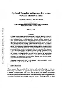
distribution over unknown variables given the data. Many methods in machine learning that are not originally graphical models, can be reinterpreted or transformed into the framework. This allows one to combine different methods in a principled manner, as well as to reuse ideas and software between sometimes surprisingly different applications. Latent variable models aim at explaining the observed data by supplementing it with unknown factors or a hidden state. The idea is that even if the regularities in the data itself are difficult to find, the dependencies between latent variables and observations are simpler, given that a proper representation is found. Model parameters and latent variables can be solved at the same time in the framework of graphical models. Basic tasks in graphical models, such as inference and learning, have been solved for decades, but relaxing the strict assumptions such as linearity of the dependencies or that the data comes in uniform samples, is a challenging and an active field of research. This thesis studies and introduces several extensions to the well-known existing graphical models. This thesis consists of an introductory part, whose structure is shown in Figure 1.1, and nine publications described in Section 1.3.

1.1

Background

Expert systems (see for example the book by Giarratano and Riley, 1994) were popular in the artificial intelligence (AI) community in the 70s. They consist of simple rules of thumb in the form of if. . . then. . . , such as if burglar or earthquake then alarm. A specialist in the field constructs a number of rules for a narrow problem domain, and an inference engine could apply the rules to an initial set of facts to obtain answers. The rules form a network where the output of a rule can be used as an input for another rule. In the simplest case, the rules are restricted to propositional calculus and truth values are binary, that is, simple statements are either true or false. Many methods in the field of AI and machine learning can be seen as extensions of expert systems in different directions. In some cases the chain of reasoning from the initial facts to answers is very long. If there is a constant number of options at each step, the size of the solution space grows exponentially and the problem becomes intractable. Chess is a typical example of such a problem. Searching (and planning) (see book by Russell and Norvig, 1995) aims at finding the optimal solution as fast as possible, and finding

1.1. Background

15

Chapter 1 Introduction

Chapter 2 Bayesian probability theory Chapter 5 Inductive logic programming Chapter 3 Graphical models background contribution Chapter 4 Variational learning of nonlinear graphical models

Chapter 6 Statistical relational learning

Chapter 7 Discussion

Figure 1.1: Dependency structure of the chapters of the thesis.

a reasonable solution in case the problem is simply too large. In this thesis, the reasoning chains are small enough so that the full structure can be always explored, but search appears in the space of solution structures, that is, on a different level of abstraction. Fuzzy logic (see book by Klir and Yuan, 1995) extends the truth values of expert systems into a continuum between 0 and 1, for instance an apple might be somewhat red or a person might be somewhat asleep. Fuzzy logic is an internally consistent body of mathematical tools but fuzzy truth values should not be interpreted as measures of uncertainty (Dubois and Prade, 1993). For instance, assume that the truth value of the event A, catching the bus, is 0.5, then the truth values of A ∧ A and A ∧ ¬A are the same in fuzzy logic. One can imagine a person being both somewhat asleep and somewhat awake at the same time, but somewhat catching a bus does not make sense. This simple example shows that fuzzy logic alone is not enough in an uncertain world. Section 4.1.5 discusses how fuzzy

16

1. Introduction

concepts can, in some sense, be brought into the probabilistic framework instead. Replacing truth values of expert systems with probabilistic variables leads to graphical models (Pearl, 1988; Neapolitan, 2004; Bishop, 2006). Graphical models can perform inferences such as “even though I heard an alarm, the probability of a burglar entering the house is fairly small because I noticed an earthquake that can also trigger the alarm.” Most expert systems would have problems using rules in both directions like in this case. Graphical models combine graph theory with probability theory. Both the structure of the graph and the parameters determining the probabilities can be learned from data. Graphical models form the basis for this work so they will be described in Chapter 3. Sometimes facts are viewed as states and rules are viewed as actions. In some cases things do not change much, for example searching becomes planning with exactly the same algorithms. Graphical models generalise to influence diagrams (Pearl, 1988). The most important concern is to keep track of what information is available to the decision maker at the time of decision. The goal of the decision maker is to maximise utility that it receives after the decisions. Decision theory is reviewed in Section 2.4. Perhaps the best known artificial neural network, the multi-layer perceptron (MLP) network (Haykin, 1999), can be related to expert systems, too. MLP network concentrates on a single if x then y rule where x and y are vectors of real values. The task is to learn a nonlinear dependency based on data. An MLP network can be constructed as a graphical model with nonlinear dependencies, allowing for new functionality, as described in Chapter 4. Latent variable models assume unknown source signals (also called factors, latent or hidden variables, or hidden causes) to have generated the observed data through an unknown mapping or process. The goal of learning is to identify both the source signals and the unknown generative mapping (or process). The success of a specific model depends on how well it captures the structure of the phenomena underlying the observations. Various linear models have been popular (see Hyvärinen et al., 2001), because their mathematical treatment is fairly easy. However, in many realistic cases the observations have been generated by a nonlinear process. Learning of a nonlinear latent variable model is a challenging task, because it is computationally much more demanding and flexible models require also strong regularisation. Variational Bayesian methods, described in Section 4.1, qualify for both computational efficiency and regularisation. Yet another direction to extend basic expert systems is to replace propositional calculus by first-order logic. The results are still called expert systems or logic programmes. One of the inference engines for first-order logic is Prolog (Sterling

1.2. Contributions of the thesis

17

and Shapiro, 1994). It is also possible to learn logic programmes from relational data. This is called inductive logic programming (Lavrac and Dzeroski, 1994; De Raedt, 2005). First-order logic allows for handling rich internal structure such as samples with a varying internal structure or links between samples. Logic programming and inductive logic programming are described in Chapter 5 and further combined with graphical models in Chapter 6.

1.2

Contributions of the thesis

Graphical models provide a good framework for machine learning and artificial intelligence. Graphical models are going to be extended, based on approximate Bayesian inference, into a system that can plan, infer, and interact with its environment using both discrete and continuous variables as well as structured representations. The concrete steps that have been taken in this work can be summarised as follows: • A novel framework where Bayesian networks may include nonlinear dependencies and algorithms for variational Bayesian learning are automatically derived. • An extension of hidden Markov models to deal with sequences of structured symbols rather than characters, with four relevant algorithms and an applications in the domain of bioinformatics. • The first graphical model that can handle both nonlinear dependencies and relations. • An extension of a method for learning nonlinear state-space models to control. • A novel algorithm for inference in nonlinear state-space models that is both efficient and reliable. • A study of methods for handling corrupted or inaccurate values in data. • A study of some latent variable models based on their capability of reconstructing missing values in data.

18

1. Introduction

Publication I Building blocks for variational Bayesian learning of latent variable models

Publication III Partially observed values

Publication IV Learning nonlinear state−space models for control

Publication VI Nonlinear relational Markov networks with an application to the game of Go

Publication II Missing values in hierarchical nonlinear factor analysis

Publication V State inference in variation Bayesian nonlinear state−space models

Publication IX ’Say EM’ for selecting probabilistic models for logical sequences

Publication VII Logical hidden Markov models

Publication VIII Towards discovering structural signatures of protein folds based on logical hidden Markov models

Figure 1.2: Publications of the thesis. Journal articles have two frames and conference papers just one. Relationships are shown as edges that are undirected since there is no clear causality.

1.3

Contents of the publications and author’s contributions

The titles of the nine publications of this thesis and their relationships are shown in Figure 1.2. Publication I introduces a framework for creating graphical models from simple building blocks. It is based on variational Bayesian learning, and unlike other such frameworks, it can model nonlinearities and nonstationary variance. Once the user defines the model structure, the algorithms for learning and inference are automatically derived. The present author developed a part of the framework, carried out a small part in the implementation, made two of the three experiments and wrote a large part of the paper. Well-founded handling of missing values is one of the advantages of Bayesian modelling. Publication II studies the reconstruction of missing values in nonlinear factor analysis. The present author made the implementation, ran the experiments, and wrote most of the paper under the guidance of Dr. Harri Valpola. Values in the data are often either observed, or missing, but some cases fall in between: Sometimes it is known that a measurement is inaccurate, or perhaps there is only a lower bound. Publication III studies handling and reconstruction

1.3. Contents of the publications and author’s contributions

19

of such partially observed values in the variational Bayesian framework. It also brings up a situation where the cost function of the variational Bayesian learning can diverge to negative infinity. It can be solved using partially observed values or by adding virtual noise in the data. Publication IV applies a state-of-the-art method from machine learning to the problem of nonlinear model-predictive control. Three different control schemes are studied, one is based directly on the learned neural network, the second one is the traditional nonlinear model-predictive control, and the third one is based on Bayesian inference. The present author designed the novel control scheme and wrote a large part of the paper. The control application brought up a setting to which none of the tested inference algorithms for nonlinear state-space models suited well. Publication V introduces a novel algorithm that both converges reliably and is still fast. The present author designed the algorithm and wrote a large part of the paper. The last four publications involve relations. Publication VI gives the first extension of graphical models to both nonlinear and relational direction at the same time. The relations in the data define a structure for a graphical model where unknown variables can then be inferred using variational Bayesian methods. The novel method is applied to the analysis of the board game Go. Hidden Markov models (HMMs) are very popular for analysing sequential data. Logical hidden Markov models (LOHMMs) extend traditional hidden Markov models to deal with sequences of structured symbols in the form of logical atoms, rather than characters. Publication VII formally introduces LOHMMs and presents efficient solutions to the three central inference problems for LOHMMs: evaluation, most likely hidden state sequence and parameter estimation. The idea came from Prof. Luc De Raedt whereas Dr. Kristian Kersting and the present author jointly formalised and implemented the LOHMMs. The present author’s contribution in experimentation and writing were minor. In Publication VIII, LOHMMs are applied to the domain of bioinformatics. The task was to extract structural signatures of folds for classes of proteins according to the classification scheme SCOP. The results indicate that LOHMMs possess several advantages over other methods. The present author took part in the design, implementation, experimentation, and writing. The increase of descriptive power of LOHMMs over HMMs comes at the expense of a more complex model selection problem, since different abstraction levels need to be explored. Publication IX presents a novel algorithm for choosing the model structure. The effectiveness of the algorithm is confirmed both theoretically and

20

1. Introduction

by experimentation with real-world unix command sequence data. The work was done jointly by Dr. K. Kersting and the present author.

Chapter 2

Bayesian probability theory Bayesian probability theory (Jaynes, 2003; MacKay, 2003; Pearl, 1988) defines probabilities to be subjective. Probabilities measure the credibility of an event so they can depend on the subjects prior knowledge, and they are updated based on observations. Say, you toss a coin and cover it with your hand without looking. The probabilities of heads or tails are even. When you peek under your hand, only the information available for you changes. For other people, the chances are still even. Bayesian probability theory gives a well-founded methodology for handling uncertainty. Given a model that describes the mutual dependencies of random variables, Bayesian probability theory can then be used to infer all the unknown variables. This chapter gives an introduction to the theory and to practicalities of Bayesian treatment of uncertainty from the machine-learning point of view.

2.1

Representations of data and belief

This thesis deals with three types of representational elements: discrete values, continuous values, and relations. This applies to both internal beliefs of the system and observations (or data). Other types of data should be possible to convert to them in a more or less sensible manner. Anderberg (1973) discusses the representations in detail, excluding relations. For categorical variables, only a finite number of values is possible. For instance, 21

22

2. Bayesian probability theory

the blood type of a person is one of four possibilities. A coin toss has two possibilities. The alphabet has 26 letters. Text is often processed by giving a discrete label to each known word. The measured sound pressure in a room is an example of a continuous value or a real number. Most physical measurements come as continuous values, such as measuring the time, weight, length, or temperature. Also the sensory systems in living organisms and robots produce continuous values. Digital cameras and scanners convert images into data where the image is divided into small square pixels that have a constant colour. The colours are described by three numbers, the red, green, and blue intensities. Sound waves can be represented as a sequence of air pressure values, like in CDs. Note that even though values are always represented with limited accuracy in computers, in theory they are handled as real numbers. Discrete numerical variables, such as the number of children, can be processed as categorical data by making a finite number of categories such as 0,1,2,3,4,5+. The other option is to reinterpret the ordinal value as a continuous value. This is often done by people, too. We have no difficulties in understanding a statement such as “Finnish women give birth to 1.7 children on average”. Section IV B of Publication III studies and solves a problem originating from a conversion of discrete to continuous values. The third type of representation, relations, is rather different from the other two. Relations are used to relate objects to one another. Codd (1970) wrote a significant paper about general relational databases. The basic idea is that access to the data is unaffected by the internal representation. This becomes important when more and more different types of data are integrated together into a common databank. Relational databases have become a standard. The universal model for data is basically a set of tables where different columns are different attributes that can be of varying type, and rows are objects. Values in the table may include identifiers that point to other rows of the same or another table. For example, a molecule can be represented as two tables, where the first one lists all atoms with their identifiers and attributes, and the second table lists all bonds, with identifiers of the involved atoms and the attributes of the bond. Similar representation applies to web pages, where instead of bonds, the second table lists links. As the biological senses never produce identifiers directly, they have to be created by the mind. For example when a predator tries to catch its pray by wearing it down, it is important for the chaser to stick to the same target even if it cannot be recognised from the herd. Also, to know the structure of a molecule, one has to know which atoms are connected with bonds even if the atoms as such

2.2. The Bayes rule and the marginalisation principle

23

are indistinguishable. Both cases can be solved by giving an implicit or explicit identifier for the prey or atom. Pointers are the identifiers used in computer code to refer to different parts of the memory, and thus to different objects. In Bayesian analysis, the belief or uncertainty about variables is represented with probabilities. The probability of an event A given prior knowledge B is written as P (A | B). Similar notation can be used when A is a discrete variable: P (A | B) denotes the probability distribution of A given B. Continuous probability distribution can be represented with a probability density function (pdf) p(·). The actual probability is an integral over the pdf. It is also called probability mass, using an analogy from physics. For exampleRthe probability of an event A < 0 0 given B can be computed as P (A < 0 | B) = −∞ p(A|B)dA.

The rest of the chapter is written for continuous values, but rewriting the integrals as sums produces the corresponding formulas for discrete values. The treatment of relations is left to Chapters 5 and 6.

2.2

The Bayes rule and the marginalisation principle

The Bayes rule was formulated by reverend Thomas Bayes in the 18th century (Bayes, 1958). It can be derived from very basic axioms (Cox, 1946). The Bayes rule tells how to update ones beliefs when receiving new information. In the following, H stands for the assumed model, X stands for observation (or data), and Θ stands for unknown variables. p(Θ | H) is the prior distribution, or the distribution of the unknown variables before making the observation. The posterior distribution is p(Θ | X, H) =

p(X | H, Θ)p(Θ | H) . p(X | H)

(2.1)

The term p(X | H, Θ) is called the likelihood of the unknown variables given the data and the term p(X | H) is called the evidence (or marginal likelihood) of the model. The marginalisation principle specifies how a learning system can predict or generalise. The probability of observing A with prior knowledge of X, H is p(A | X, H) =

Z

p(A | Θ, X, H)p(Θ | X, H)dΘ.

(2.2)

24


It means that the probability of observing A can be acquired by summing or integrating over all different explanations Θ. The term p(A | Θ, X, H) is the probability of A given a particular explanation Θ and it is weighted with the probability of the explanation p(Θ | X, H). Using the marginalisation principle, the evidence term can be written as Z p(X | H) = p(X | Θ, H)p(Θ | H)dΘ.

(2.3)

This emphasises the role of the evidence term as a normalisation coefficient. It is an integral over the numerator of the Bayes rule (2.1). Sometimes it is impossible to compute the integral exactly, but fortunately it is not always necessary. For example, when comparing posterior probabilities of different instantiations of hidden variables, the evidence cancels out.

2.3

Structure among unknown variables

For getting a model that is useful in new situations, i.e. having generalisation ability, some structure among the unknown variables Θ needs to be assumed. A typical structure in machine learning is a division of unknown variables Θ into parameters θ and latent variables S, Θ = (θ, S). The distinction is that parameters θ are shared among data samples, but there are separate latent variables for each data sample. Thus, the number of latent variables grows linearly with data size while the number of parameters stays the same. The latent variables can be thought of as the internal state of a system. Sometimes computing the posterior distribution over the parameters θ is called Bayesian learning, leaving the term Bayesian inference to only refer to computing the posterior distribution of latent variables S. Graphical models, described in Chapter 3, provide a formalism for defining the exact structure of dependencies. The fundamental idea is that a complex system can be built by combining simpler parts. A graphical model is a graph whose nodes represent random variables and edges represent direct dependencies.

2.4

Decision theory

Decision theory (see book by Dean and Wellman, 1991) was first formulated by Blaise Pascal in the 17th century. When faced with a number of actions A, each

2.5. Approximations

25

with possibly more than one possible outcome B with different probabilities P (B | A), the rational choice is the action that gives the highest expected value U (A): Z U (A, B)P (B | A), (2.4) U (A) = B

where U (A, B) is the value of action A producing the outcome B. Daniel Bernoulli refined the idea in the 18th century. In his solution, he defines a utility function and computes expected utility rather than expected financial value. For example, people tend to insure their property even though the expected financial value of the decision is negative (after all, insurance business must be profitable for the insurance companies). This is explained by the fact that in case of losing one’s whole property, every euro is more important (has more utility). Bayesian decision theory (see book by Bernardo and Smith, 2000) works in situations where the outcomes of actions are unknown but one still has to make decisions. One simply chooses the action with highest expected utility over the predictive distribution of outcomes. Bayesian decision theory does not just give a way to make actions but it is actually the only coherent way of acting. This can be shown using a so-called Dutch book argument (Resnik, 1987). A Dutch book is a set of odds and bets which guarantees a profit, no matter what the outcome of the gamble. A Dutch book can never be made against a Bayesian decision maker, and if decisions are such that a Dutch book cannot be made against the decision maker, the decisions can always be interpreted to be made by a Bayesian decision maker. Decision theory has a clear connection to control theory. (Dean and Wellman, 1991) The control that minimises a certain cost functional is called the optimal control (see book by Kirk, 2004). When the control cost is used as the negative utility −U (·), decision theory provides optimal control, even under uncertainty (stochastic control). Section 4.3.2 and Publication IV apply Bayesian decision theory for control in nonlinear state-space models.

2.5

Approximations

The Bayesian probability theory and decision theory sound too good to be true: They solve learning, inference, and decision making optimally. Unfortunately, the posterior probability distribution cannot be handled analytically except in the simplest examples. To solve the integrals in Equations (2.2), (2.3), and (2.4), one must resort to some kind of approximations. There are three common classes of approximations: point estimates, sampling, and variational approximations.

26


6

2 4

1 2

0

0

−1

−2

−2

−4

−2

−1

0

1

2

−2

0

2

4

6

8

Figure 2.1: Posterior distributions of x and y are shown in black contours. Maximum a posterior estimate is plotted as a red star, Bayes estimate (or the expectation over the posterior) is plotted as a red circle. Variational Bayesian solution with a Gaussian posterior approximation with diagonal covariance is shown in blue as a dot surrounded by ellipses. Left: model p(z) = N (z; xy, 0.02), observation z = 1, priors p(x) = N (x; 0, 1), p(y) = N (y; 0, 1). Right: model p(z) = N (z; y, exp(−x)), observation z = 2, priors p(x) = N (x; −1, 5), p(y) = N (y; 0, 5).

Figure 2.1 shows two posterior distributions. The models are not particularly meaningful (having just two unknown variables), but they are chosen to highlight differences in various posterior approximations, which are described in the following.

2.5.1

Point estimates

Point estimates use a single representative value to summarise the whole posterior distribution. The maximum likelihood (ML) estimate (or solution) for the unknown variables Θ is the point in which the likelihood p(X | Θ, H) is highest. The maximum a posteriori (MAP) estimate is the one with highest posterior probability density p(Θ | X, H). Note that a common and even simpler criterion, the mean square error, is equivalent to the ML estimate assuming Gaussian noise with constant variance (Bishop, 1995). An iterative learning algorithm is said to overlearn the training data set, when its

2.5. Approximations

27

Figure 2.2: A sixth order polynomial is fitted to 10 data points. Left: Maximum likelihood solution. Right: Bayesian solution. The three curves present 5%, 50% and 95% fractiles.

performance with unseen test data starts to get worse during the learning with training data (Haykin, 1999; Bishop, 1995; Chen, 1990). The system starts to lose its ability to generalise. The same can happen when increasing the complexity of the model. The model is said to overfit to the data. In this case the model becomes too complicated and concentrates on random fluctuations in the data. The left subfigure of Figure 2.2 shows an example of overfitting. When the model is too simple or the learning is stopped too early, the problem is called underfitting or underlearning respectively. Balancing between over- and underfitting has perhaps been the main difficulty in model building. There are several ways to fight overfitting and overlearning (Haykin, 1999; Bishop, 1995; Chen, 1990). A popular method is to select the best time to stop learning or the best complexity of a model by cross-validation (Stone, 1974; Haykin, 1999). Part of the training data is left for validation and the models are compared based on their performance with the validation set. The problems of overlearning and overfitting are mostly related to point estimates. The example in Figure 2.2 is solved by using the whole posterior distribution instead of a single solution. The use of a point estimate is to approximate integrals so it should be sensitive to the probability mass rather than to the probability density. Unfortunately, ML and MAP estimates are attracted to high but sometimes narrow peaks. Figure 2.3 shows a situation, where search for the MAP solution first finds a good representative of the probability mass, but then moves to the highest peak which is on the border. This type of situation seems to be very common and the effect becomes stronger, when the dimensionality increases. Appendix D of

28


Figure 2.3: A hypothetical posterior pdf. A point estimate could first find a good representative of the probability mass, but then overfits to a narrow peak. Publication I gives an example where point estimates fail completely.

2.5.2

The Laplace approximation

Compared to the point estimates, a more accurate way to approximate the integrals in Equations (2.2), (2.3), and (2.4) is to use the Laplace approximation (see Bishop, 1995; MacKay, 2003). The basic idea is to find the maximum of the function to be integrated and apply a second order Taylor series approximation for the logarithm of that function. In case of computing an expectation over the posterior distribution, the maximum is the MAP solution and the second order Taylor series corresponds to a Gaussian distribution for which integrals can be computed analytically. The Laplace approximation can be used to select the best solution in case several local maxima have been found since a broad peak is preferred over a high but narrow peak. Unfortunately the Laplace approximation does not help in situations where a good representative of the probability mass is not a local

2.5. Approximations

29

maximum, like in Figure 2.3. Laplace approximation can be used to compare different model structures successfully. It can be further simplified by retaining only the terms that grow with the number of data samples. This is known as the Bayesian information criterion (BIC) by Schwarz (1978). Publication IX uses BIC in structural learning of logical hidden Markov models.

2.5.3

Expectation-maximisation algorithm

The expectation-maximisation (EM) algorithm (Dempster et al., 1977; Neal and Hinton, 1999; MacKay, 2003) can be seen as a hybrid of point estimates and accurate Bayesian treatment. Recall the division of unknown variables Θ into parameters θ and latent variables S in Section 2.3. EM uses point estimates for parameters θ and distributions for latent variables S. The idea is that updating is easy when these two are updated alternately. In the E-step, given certain values for parameters θ, the posterior distribution of latent variables S can be solved. In the M-step, the parameters θ are updated to maximise likelihood or posterior density, given a fixed distribution over latent variables S. Originally the EM algorithm was used for maximum likelihood estimation in the presence of missing data. Later it was noted that latent variables can be seen as missing data and priors can be included to get the MAP estimate. Note that EM does not only yield a posterior approximation, but also gives practical rules for iterative updates. In a sense, EM is a recipe or meta-algorithm which is used to devise particular algorithms using model-specific E and M steps. EM is popular for its simplicity but speeding up the EM algorithm has been a topic of interest since its formulation (Meng and van Dyk, 1995). Petersen et al. (2005) analyse slowness in the limit of low noise (see also Raiko, 2001, Figure 6.1). It can be more effective to update both S and θ at the same time by for instance using gradient-based algorithms (for comparison, see Kersting and Landwehr, 2004), hybrids of EM and gradient methods (Salakhutdinov et al., 2003), or complementing alternative updates with line search (Honkela et al., 2003). Also, there are many benefits from choosing a posterior approximation that is a distribution instead of a single set of values, such as robustness against overfitting and well-founded model selection. The EM algorithm is adapted for parameter estimation of logical hidden Markov models in Publication VII.

30

2.5.4


Markov chain Monte Carlo methods

Markov Chain Monte Carlo (MCMC) methods (Gelman et al., 1995; MacKay, 2003) approximate the posterior distribution by generating a sequence of random samples from it. The integrals in Equations (2.2) and (2.4) are approximated by summing over the samples. There are many algorithms for the actual sampling, the best-known being Metropolis-Hastings algorithm and the Gibbs sampler (MacKay, 2003; Haykin, 1999). A popular method by Neal (2001) for approximating the integral in Equation (2.3) is known as annealed importance sampling. Gibbs sampling introduced by Geman and Geman (1984) is as follows. Known variables are fixed to their values and unknown variables are given some initial values. The value of some unknown variable is updated by sampling from its conditional probability distribution assuming all the other variables fixed. This is done repeatedly for all unknown variables. First samples are discarded but the rest represent the posterior distribution, that is, expected values are estimated as sample means and so on. Assuming that all states can be reached by this process, the limiting distribution of the process is the true posterior distribution. Gibbs sampling is used for instance in the BUGS project by Spiegelhalter et al. (1995) and by Hofmann and Tresp (1996, 1998). Sampling methods are very general and very accurate assuming enough computational resources. Unfortunately they are often computationally very demanding. Also, it is difficult to say when the process has converged (MacKay, 2003). For instance in the left subfigure of Figure 2.1, it is astronomically rare that the Gibbs sampler would find its way from one solution mode to the other. Expectation over the samples for the parameters is often used for interpretation (including visualisation) purposes, or for fast application phase after learning. This can be problematic when the posterior distribution is multi-modal. Latent variable models often exhibit symmetries with respect to permuting the latent variables or changing signs of pairs of variables as in the left subfigure of Figure 2.1. In this case, the expected values are completely meaningless.

2.5.5

Variational approximations

Variational Bayesian (VB) methods fit a distribution of a simple form to the true posterior density. VB is sensitive to probability mass rather than to probability density. This gives it advantages over point estimates: it is robust against overfitting, and it provides a cost function suitable for learning model structures. If the true posterior has more than one mode (or cluster), VB solution finds just

2.5. Approximations

31

one of them, as shown in the left subfigure of Figure 2.1. VB provides a criterion for learning, but leaves the algorithm open. Variational Bayesian learning will be described in more detail in Section 4.1. Depending on the form of the approximating distribution, variational Bayesian density estimates can be computationally almost as efficient as point estimates. Roberts and Everson (2001) compared Laplace approximation, sample based, and variational Bayesian learning in an independent component analysis problem on music data. The sources were well recovered using VB learning and the approach was considerably faster than the sample-based methods. Beal and Ghahramani (2003) compared VB, BIC, and annealed importance sampling in scoring model structures. VB gave a good compromise being a lot more accurate than BIC, and about a hundred times faster than sampling with comparable accuracy. Expectation propagation by Minka (2001) is closely related to VB. A parametric distribution is fitted to the true posterior, but the measure of misfit is different. It aims at a posterior approximation that contains the whole solution. VB approximation works the other way around: the whole approximation should be contained within the solution. The difference is most apparent in cases where the posterior is multi-modal, like in the left subfigure of Figure 2.1. An approximation that contains both modes, also contains a lot of areas with low probability in between. In such cases it is reasonable to select a single mode. Expectation propagation is an algorithm whereas VB is a criterion. Unfortunately the convergence of the expectation propagation algorithm cannot be guaranteed.

Chapter 3

Graphical models Graphical models (Pearl, 1988; Jensen et al., 1990; Cowell et al., 1999; Neapolitan, 2004; Bishop, 2006; Murphy, 2001) provide a formalism for defining the structure for a probabilistic model. A graphical model is a graph whose nodes represent random variables and edges represent direct dependencies. The models presented here vary mostly in whether they are static or dynamic and whether the variables are discrete or continuous valued. Graphical models have evolved from being a mere academic curiosity into a popular field of research with a huge number of applications. The applications range from network engineering to bioinformatics. All the models and methods studied in this thesis can be seen as extensions of these basic models, which are therefore introduced here.

3.1

Well-known graphical models

In the following, well-known graphical models are described. Most of them have been invented before the general framework and thus, the graphical model framework can be seen as a way to view all of these methods as instances of a common formalism. Using the shared formalism, developments in one field are easier to transfer to others (Jordan, 1999). 32

3.1. Well-known graphical models

earthquake

33

burglary

report

earthquake

report

alarm

neighbour 1 calls

neighbour 2 calls

earthquake report earthquake

burglary

alarm

neighbour 1 calls

neighbour 2 calls

alarm neighbour 1 calls

burglary alarm

alarm neighbour 2 calls

Figure 3.1: Top left: Bayesian network for the alarm example. Top right: A Markov network formed by connecting all parents that share a common child and removing edge directions. Bottom: The corresponding join tree whose nodes correspond to cliques of the Markov network.

3.1.1

Bayesian networks

Let us study an example by Pearl (1988). Mr. Holmes receives a phone call from his neighbour about an alarm in his house. As he is debating whether or not to rush home, he remembers that the alarm might have been triggered by an earthquake. If an earthquake had occurred, it might be on the news, so he turns on his radio. The events are shown in Figure 3.1. Marking the events earthquake by E, burglary by B and so on, the joint probability can be factored into P (E, B, R, A, N1 , N2 ) = P (E)P (B | E)P (R | E, B)P (A | E, B, R)P (N1 | E, B, R, A)P (N2 | E, B, R, A, N1 ) = P (E)P (B)P (R | E)P (A | E, B)P (N1 | A)P (N2 | A). (3.1) The first equation is just basic manipulation of probabilities and the second equation represents conditional independencies. For instance, the probability of an earthquake report on the radio R does not depend on whether there is a burglary B or not, given that we know whether there was an earthquake or not, so P (R | E, B) = P (R | E).

34

3. Graphical models

A=true A=false

N1 =true 0.7 0.001

N1 =false 0.3 0.999

Table 3.1: The conditional probability table describing P (N1 | A).

The graphical representation of the conditional probabilities depicted in the top left subfigure of Figure 3.1 is intuitive: arrows point from causes to effects. Note that the graph has to be acyclic, no occurrence can be its own cause. Loops, or cycles when disregarding directions of the edges, are allowed. Assuming that the variables are discrete, the conditional probabilities are described using a conditional probability table that lists probabilities for all combinations of values for the relevant variables. For instance, P (N1 | A) is described in Table 3.1. Recalling the notation from Section 2.3, the numbers in the conditional probability table are parameters θ while unobserved variables in the nodes are S. Inference in Bayesian networks solves questions such as “what is the probability of burglary given that neighbour 1 calls about the alarm?” Approximate inference methods such as sampling (see Section 2.5.4) can be used, but in relatively simple cases, also exact inference can be done. For that purpose, we will form the join tree of the Bayesian network. First, we connect parents of a node to each other, and remove all directions of the edges, (see top right subfigure of Figure 3.1). This is called a Markov network. Next, we find all cliques (fully connected subgraphs) of the Markov network. Then we create a join tree1 where nodes represent the cliques in the Markov network and edges are set between nodes who share some variables (see bottom subfigure of Figure 3.1). We can rewrite the joint distribution in Equation 3.1 as

P (E, B, R, A, N1 , N2 ) =

P (R, E)P (E, B, A)P (A, N1 )P (A, N2 ) , P (E)P (A)P (A)

(3.2)

where the numerator is a product of distributions of nodes in the join tree and the denominator is the product of the distributions of the edges of the join tree. Then the inference question “what is the probability of burglary given that neighbour 1 calls about the alarm?” is solved by substituting N1 = true and marginalising

1 We

assume for now that the join tree is really a tree.


35

the uninteresting variables away: P (B, N1 = true) P (N1 = true) ∝ P (B, N1 = true) X P (E, B, R, A, N1 = true, N2 ) =

P (B | N1 = true) =

E,R,A,N2

=

X

E,R,A,N2

P (R, E)P (E, B, A)P (A, N1 = true)P (A, N2 ) , P (E)P (A)P (A) (3.3)

where ∝ means “proportional to”. The constant P (N1 = true) can be ignored if the resulting distribution is normalised in the end. Summing over all the latent variables is often prohibitively computationally expensive, so better means have been found. For efficient marginalisation in join trees, there is an algorithm called belief propagation (Pearl, 1988) based on message passing. First, any one of the nodes in the join tree is selected as a root. Messages π are sent away from the root and messages λ towards the root. The marginal posterior probability of a node X in the join tree given observations e is decomposed into two parts: P (X | e) ∝ P (X | eanc(X) )P (edesc(X) | X) = π(X)λ(X),

(3.4)

where eanc(X) and edesc(X) are the observations in the ancestor and descendant nodes of X in the join tree accordingly. The messages can be computed recursively by X π(X) = P (X | Y )π(Y ) (3.5) Y

λ(Y ) =

Y

λj (Y )

(3.6)

λ(X)P (X | Y )

(3.7)

j

λX (Y ) =

X X

where Y is the parent of X in the join tree and j are its children, including X. The message π for the root node is set to the prior probability of the node, and the messages λ are set to uniform distribution for the unobserved leaf nodes. The belief propagation algorithm extended for logical hidden Markov models in Publication VII.

36

3. Graphical models

Returning to the example in Equation 3.2 and selecting node (E, B, A) as the root of the join tree, the necessary messages are π(E, B, A) = P (E, B, A) X λ(R,E) (E, B, A) = λ(R)P (R | E, B, A)

(3.8) (3.9)

R

λ(A,N1 ) (E, B, A) =

X

λ(N1 )P (N1 | E, B, A)

(3.10)

λ(N2 )P (N2 | E, B, A).

(3.11)

N1

λ(A,N2 ) (E, B, A) =

X N2

Since λ(R) and λ(N2 ) are uniform (unobserved leaf nodes), it is easy to see that λ(R,E) (E, B, A) and λ(A,N2 ) (E, B, A) are also uniform and can thus be ignored. We get X P (B | N1 = true) = π(E, B, A)λ(E, B, A) E,A

=

X

P (E, B, A)λ(A,N1 ) (E, B, A)

E,A

=

X

P (E, B, A)P (N1 = true | E, B, A)

E,A

=

X

P (E)P (B)P (A | E, B)P (N1 = true | A).

(3.12)

E,A

For the inference to be exact, the join tree must not have loops (like the name implies). Loopy belief propagation by Murphy et al. (1999) uses belief propagation algorithm regardless of loops. Experiments show that in many cases it still works fine. The messages are initialised uniformly and iteratively updated until the process hopefully converges. It is also possible to find an exact solution by getting rid of loops at the cost of increased computational complexity. This happens by adding edges to the Markov network. Bayesian networks can manage continuous valued variables, when three simplifying assumptions are made (Pearl, 1988). All interactions between variables are linear, the sources of uncertainty are normally distributed, and the causal network is singly connected (no two nodes share both common descendants and common ancestors). Instead of tables, the conditional probabilities are described with linear mappings. Posterior probability is Gaussian. Bayesian networks are static, that is, each data sample is independent from others. The extension to dynamic (or temporal) Bayesian networks (see Ghahramani,


37

1998) is straightforward. Assume that the data samples x, e.g. x = (E, B, R, A, N1 , N2 ), are indexed by time t. Each variable can have as parents variables of sample x(t−1) in addition to the variables of the sample itself x(t). Hidden Markov models (see Section 3.1.5) are an important special case of dynamic Bayesian networks. Linearity assumption can be relaxed when some approximations are made. Section 4.4 and Publication I present such a framework based on variational Bayesian learning. There are also other approaches. Hofmann and Tresp (1996) study Bayesian networks with nonlinear conditional density estimators. Inference is based on Gibbs sampling and learning is based on cross-validated maximum a posteriori estimation.

3.1.2

Markov networks

Markov networks (Pearl, 1988), historically also known as Markov random fields, are undirected graphical models. A Markov network does not commit on whether A caused B, it is interested only whether there is a dependency or not. A popular application is images where pixels are variables and edges are drawn between neighbouring pixels. Since inference in Bayesian networks was explained by first transforming it into a Markov network, inference in Markov networks does not require much additional attention. We just start directly from the undirected graph, like in the top right subfigure of Figure 3.1. The joint density can be written directly as in Equation 3.2, but the standard way of writing the joint distribution is different. The joint distribution is proportional to the product of potentials ψ over the cliques of the network, for example: P (E, B, R, A, N1 , N2 ) ∝ ψ(R, E)ψ(E, B, A)ψ(A, N1 )ψ(A, N2 ).

(3.13)

Like Bayesian networks, Markov networks can manage continuous values with same simplifying assumptions that can be relaxed by resorting to approximations. Hofmann and Tresp (1998) introduce nonlinear Markov networks. Each continuous valued variable xi is modelled using all of its neighbours Bi in the network. The modelled conditional densities pM (xi | Bi ) can be directly used for Gibbs sampling. The complete likelihood function involves some integrals which cannot be solved in closed form but need to be approximated numerically. Taskar et al. (2002) introduce relational Markov networks (RMN) where the structure of the Markov network is defined by the relational data. Each variable might have a different number of neighbours, but generalisation is possible due to shared clique potentials.

38

3. Graphical models

s 1(t)

s2(t)

a11

a a12 a21 a22 a31 32 x1(t) x2(t) x3(t) Figure 3.2: Graphical representations of factor analysis, principal component analysis, and independent component analysis are the same. Latent variables in the top layer are fully connected to the observations in the bottom layer. In this case, the vectors s(t) are two dimensional and x(t) are three dimensional.

Section 6.3 and Publication VI extend these ideas into nonlinear relational Markov networks.

3.1.3

Factor analysis and principal component analysis

Factor analysis (Harman, 1967; Kendall, 1975; Hyv¨ arinen et al., 2001) (FA) can be seen as a Bayesian network consisting of two layers, depicted in Figure 3.2. The top layer contains latent variables s(t) and the bottom layer contains observations x(t). The two layers are fully connected, that is, each observation has all of the latent variables as its parents. The index t stands for the data case. The mapping from factors to data is linear2 x(t) = As(t) + n(t), or componentwise xi (t) =

X

aij sj (t) + nj (t),

(3.14)

(3.15)

j

where n(t) is noise or reconstruction error vector. Typically the dimensionality of the factors is smaller than that of the data. Factors and noise are assumed to have a Gaussian distribution with an identity and diagonal covariance matrix, 2 Note

that the data is assumed to be zero mean here to simplify the equations.


39

respectively. Recalling the notation from Section 2.3, parameters θ include the weight matrix A and noise covariance for n(t). Equation (3.14) does not fix the matrix A, since there is a group of rotations that yields identical observation distributions. Several criteria have been suggested for determining the rotation. One is parsimony, which roughly means that most of the values in A are close to zero. Another one leads to independent component analysis described in Section 3.1.4. Sections 4.2 and 4.4.2 describe extensions of factor analysis releasing from the linearity assumption of the dependency between factors and observations. Principal component analysis (PCA) (Jolliffe, 1986; Kendall, 1975; Hyvärinen et al., 2001), equivalent to the Hotelling transform, the Karhunen-Loève transform, and the singular value decomposition, is a widely used method for finding the most important directions in the data in the mean-square sense. It is the solution of the FA problem under low noise (see Bishop, 2006) with orthogonal principal components (the columns of the weight matrix A). The first principal component a1 corresponds to the line on which the projection of the data has the greatest variance:

a1 = arg max

||ξ||=1

T X

(ξ T x(t))2 .

(3.16)

t=1

The other components are found recursively by first removing the projections to the previous principal components:

ak = arg max

||ξ||=1

T X t=1

"

ξ

T

x(t) −

k−1 X i=1

!#2

ai aTi x(t)

.

(3.17)

There are many other ways to formulate PCA, including probabilistic PCA (Bishop, 1999). In practice, the principal components are found by calculating the eigenvectors of the covariance matrix C of the data C = E x(t)x(t)T

(3.18)

The eigenvalues are positive and they correspond to the variances of the projections of data on the eigenvectors. The weight matrix A is formed from the eigenvectors and it is always orthogonal.

40

3.1.4

3. Graphical models

Independent component analysis

The mixing model of independent component analysis (ICA) is similar to that of the FA (see Figure 3.2), but in the basic case with equal number of factors (or components) as observations and without the noise term. The data is thought to have been generated from independent components s(t) through a square mixing matrix A by x(t) = As(t). (3.19) The components s(t) are independent, that is, p(s1 , s2 , . . . , sn ) = p1 (s1 )p2 (s2 ) . . . pn (sn ),

(3.20)

and the assumption of Gaussianity of the components is relaxed. Assuming that at most one of the independent components is Gaussian, the model is identifiable (Comon, 1994). In the basic case, the number of components is the same as the number of observation and the components can be reconstructed from data given the mixing matrix A by s(t) = A−1 x(t). The independence of the reconstructed s(t) can then be measured for instance by the non-Gaussianity of the components or by mutual information (Hyv¨ arinen et al., 2001). ICA can thus be done by iteratively maximising such a measure. ICA has many fields of applications, such as brain imaging (Vigário et al., 1998), telecommunications (Raju et al., 2006; Ristaniemi, 2000), speech separation, and so on (Hyv¨ arinen et al., 2001). ICA can be approached from different starting points. It can be viewed as a Bayesian network when the one dimensional distributions for the components are modelled with for example mixtures-of-Gaussians (Attias, 1999, 2001; Choudrey et al., 2000; Miskin and MacKay, 2001). This is also known as independent factor analysis. Extensions to the basic ICA involve additive noise, convolutive or nonlinear mixing, and the number of components might differ from the number of observations (Hyv¨ arinen et al., 2001). Publication III studies the reconstruction of corrupted values in data by independent factor analysis.

3.1.5

Hidden Markov models

Hidden Markov models (HMMs) (Rabiner and Juang, 1986) are dynamic Bayesian networks with a certain structure. Observed data are assumed to be generated as a function of an unobserved state which is evolving stochastically in time. The


41

1.0

start

bag 0.7:t

0.3:t S(0)

S(1)

S(2)

x(1)

S(3)

coin1

x(2)

s(0)

bag

coin2 0.3:h

0.7:h

coin1 start

0.5 0.5

coin1

coin1 bag

bag coin2

coin2

coin2

s(1)

s(2)

s(3)

Figure 3.3: Graphical representations of a hidden Markov model. Top left: The corresponding Bayesian network. Top right: The transitions are represented with an arrow and annotated with transition probabilities and possible observations. Bottom: The trellis showing all the possible evolutions of states unrolled in time.

observations x(t) are conditioned on state s(t). The discrete state s(t) at time t is a latent variable and the conditional probability for a state transition P (s(t) | s(t − 1)) does not depend on t. Here we will use a non-standard formulation where the state transition is conditioned on the observation as well, that is, P (s(t) | s(t − 1), x(t − 1)). It is fairly easy to see that the two approaches are equivalent3 in representational capacity. Appendix B of Publication VII shows that the two approaches are equivalent in a setting generalised to first-order logic. Figure 3.3 shows an example of a HMM. There are two bent coins in a bag, one gives more heads and the other more tails. A person draws a coin randomly from the bag and tosses it until it lays tails up. At that point it is put back to the bag and one of the coins is drawn and tossed again. At time 0, the system is always in the start state (s(0) =start). Afterwards, it is always either in state coin1 or coin2 possibly going through an auxiliary state bag. The state being hidden (or latent) means that one does not know which coin is used, only the sequence of heads and tails is observed. 3 By either ignoring the conditioned x(t − 1) or including a copy of the observation to the hidden state.

42

3. Graphical models

The instance of belief propagation algorithm for HMMs is called the forwardbackward algorithm. In the example, this would give the probabilities for which coin was drawn from the bag at each stage. It is also possible to learn the parameters from observations, say, estimate how badly the coins are bent. That can be done using the Baum-Welch algorithm, which is the instance of EM algorithm for HMMs. Hidden Markov models are very popular for analysing sequential data. Application areas include computational biology (Koski, 2001), speech recognition (Rabiner and Juang, 1986), natural language processing (Charniak, 1993), user modelling (Lane, 1999), and robotics (Meila and Jordan, 1996). There are several extensions of HMMs such as factorial HMMs by Ghahramani and Jordan (1997), relational Markov models by Anderson et al. (2002), and extension based on tree automata by Frasconi et al. (2002). Section 6.2 and Publication VII introduce an extension of hidden Markov models to first-order logic, which generalises all of the above.

3.1.6

State-space models

Linear state-space models (see textbook by Chen, 1999) share the same structure as hidden Markov models but now the states s(t) and observations x(t) are continuous valued vectors. The conditional probabilities are represented as a linear mapping with additive Gaussian noise: s(t) = Bs(t − 1) + ns (t) x(t) = As(t) + nx (t)

(3.21) (3.22)

Note that Equation (3.22) is exactly the same as (3.14), that is, state-space models can be seen as a dynamic extension of factor analysis. The dynamics in Equation (3.21) correspond to linear dynamical systems discretised in the time domain. Again, the belief propagation algorithm has another name, and it was originally derived from a different starting point probably by a Danish statistician T.N. Thiele in 1880 and later popularised by Kalman (1960) (see also the textbook by Anderson and Moore, 1979). In the context of state-space models, belief propagation is known as the Kalman smoother. It is popular in many applications fields, including econometrics (Engle and Watson, 1987), radar tracking (Chui and Chen, 1991), control systems (Maybeck, 1979), signal processing, navigation, and robotics. In control systems, dynamics can be affected by control inputs u(t). Equation

3.2. Tasks

43

(3.21) for dynamics is replaced by s(t) = Bs(t − 1) + Cu(t) + ns (t).

(3.23)

Note that the control inputs u(t) are coming from outside the generative model. One possibility is to use feedback control (see textbook by Doyle et al., 1992), u(t) = −Kx(t − 1) + r(t),

(3.24)

but note that K and r(t) should be chosen so as to accomplish the control goal, not by inference or learning. Section 4.3 studies an extension to nonlinear state-space models where the linear mappings A and B are replaced by multi-layer perceptron networks. Section 4.3.2 and Publication IV study control in nonlinear state-space models.

3.2

Tasks

This thesis studies four tasks that can be done with graphical models: inferring the distributions for latent variables, estimating (or learning) parameters of the model, learning the structure of the model, and making decisions. Each of them is described in turn.

3.2.1

Inference

Inference is the task of computing the posterior probability over the latent variables S given a fixed set of parameters θ, the data X and the model structure H, according to the Bayes rule (Equation 2.1). The distribution is often very high dimensional and for all practical purposes it is represented as marginal distributions (see Eq. 2.2) over groups of variables. The computations are not straightforward and therefore one needs to use algorithms such as belief propagation, described in Section 3.1.1. One of the advantages of graphical models is that handling of missing values in data is straightforward and consistent. Instead of belonging to data X, missing values belong to latent variables S and their reconstructions (or posterior distributions) are inferred as any other latent variables. Reconstruction of missing values in linear and nonlinear models is studied in Section 4.1.4 and Publication II. Exact inference by belief propagation has exponential computational complexity with respect to the size of the largest clique in the Markov network (see Figure 3.1),

44

3. Graphical models

so often one needs to settle for approximated inference. In some extensions such as nonlinear state-space models described in Section 4.3, there is no analytical solution at all. Different kinds of approximate methods are described in Section 2.5.

3.2.2

Parameter learning

The task of learning the parameters of a model means that given a set of data cases or observations X and a model structure H, one can infer the distribution over the model parameters θ, found for instance in the conditional probability table in Table 3.1, in the clique potentials ψ in Equation (3.13), in the mapping A in Equation (3.14), or the transition probabilities in Figure 3.3. Parameter learning does not differ from inference in Bayesian probability theory, so the reasons for studying them separately are mostly practical. For instance in the EM algorithm, the updates of parameters and latent variables are done separately and in different ways. Also, local update rules work efficiently in parameter learning, whereas explicit propagation of information is important in state inference of dynamic systems (see Publication V). Parameter learning can be really simple. Consider learning the values in the conditional probability table for neighbour 1 calling about the alarm in case there is an alarm or not, P (N1 | A) in Table 3.1. Given data samples where we observe whether there was an alarm and whether the neighbour called or not, let us settle for a point estimate: the most likely set of parameters. The ML solution is simply to count how many times each of the four cases appear in the data and turn them into probabilities by normalising each row to sum to one.

3.2.3

Structural learning

Also the structure of the model can be learned from data. This includes adding edges between nodes and possibly new nodes. A straightforward way of learning the structure is to try out different structures H and select the one with the largest marginal likelihood P (X | H) (see Equation 2.3). Depending on the approximations, sometimes more complex models need to be explicitly penalised (MacKay, 1995b). Just like parameter learning includes inference as a subproblem, structural learning includes parameter learning as a subproblem. To measure the model evidence for a structure, parameters need to be learned. A standard way of searching is to generate candidate structures by making minimal changes in the current hy-

3.2. Tasks

45

pothesis, such as adding, deleting, or reversing an edge. Parameters of the current hypothesis can be used as a good first guess for the parameters of the candidates. In a greedy search, the best candidate is selected as the next hypothesis. Getting stuck in a local minimum can be avoided for instance by using simulated annealing by Kirkpatrick et al. (1983) (Haykin, 1999). Structural EM by Friedman (1998) speeds up structural search. The posterior distribution over the latent variables is inferred for the current hypothesis and fixed. Then, candidate hypotheses are evaluated using this distribution, that is, only the parameters are updated. As before, one of the candidates is selected as the next current hypothesis and the inference is done again. Now, instead of running EM algorithm for each candidate structure, only a single M-step of the EM algorithm is needed. Candidate evaluation is not as accurate as before, but this is easily compensated by the large speed-up. The structural learning algorithm for logical hidden Markov models, introduced in Publication IX, is based on generalised structural EM. There is a second broad class of algorithms for structural learning besides performing a search. These are known as independence-based or constraint-based algorithms. For example, Bromberg et al. (2006) discover structures of Markov networks using independence tests.

3.2.4

Decision making

The fourth task, decision making, differs a lot from the other three. The task is to select actions that maximise expected utility, as explained in Section 2.4. The actions or controls appear as external inputs in the graphical model, such as the control inputs u(t) in Section 3.1.6. Utility, like random variables, can also be decomposed into nodes. The global utility is a sum of local utilities. A utility node has as parents all the actions and random variables on which it depends. Now, the values for action nodes can be selected to maximise expected utility (Cowell et al., 1999). The resulting graph is called an influence diagram (Pearl, 1988). In model-predictive control (e.g. Eduardo Fern´ andez Camacho, 2004), actions can be selected as follows. First, some initial guess for the actions is made. Latent variables and utilities are inferred for a given sequence of actions. The gradient of total expected utility with respect to each random variable and action is propagated backwards to each action. Actions are updated in the direction of increasing utility, and the process is iterated. Application of this to control in nonlinear

46

3. Graphical models

state-space models is described in Section 4.3.2 and Publication IV.

Chapter 4

Variational learning of nonlinear graphical models This chapter describes extensions of graphical models with continuous values to the case where the linearity assumption is relaxed. These are known as nonlinear graphical models. For reasons explained in Section 2.5, nonlinear graphical model suit well to be handled using variational Bayesian methods. Section 4.1 describes variational Bayesian methods in general and the rest of the chapter describes some particular models.

4.1

Variational Bayesian methods

Variational Bayesian (VB) learning (Barber and Bishop, 1998; Hinton and van Camp, 1993; Lappalainen and Miskin, 2000; MacKay, 1995a, 2003; Jordan et al., 1999; Lappalainen and Honkela, 2000) is a fairly recently introduced (Wallace, 1990; Hinton and van Camp, 1993) approximate fully Bayesian method, which has become popular because of its good properties. Its key idea is to approximate the exact posterior distribution p(Θ | X, H) by another distribution q(Θ) that is computationally easier to handle. Typically, the misfit of the approximation is measured by the Kullback-Leibler (KL) divergence between two probability distributions q(v) and p(v). The KL 47

48

4. Variational learning of nonlinear graphical models

divergence is defined by

D(q(v) k p(v)) =

Z

q(v) ln

q(v) dv ≥ 0 p(v)

(4.1)

which measures the difference in the probability mass between the densities q(v) and p(v). Its minimum value 0 is achieved when the densities q(v) and p(v) are the same. The VB method works by iteratively minimising the misfit between the actual posterior pdf and its parametric approximation using the KL divergence. Note that VB learning defines the goal and a performance measure, but leaves the actual algorithm open. The approximating distribution q(Θ) is usually chosen to be a product of several independent distributions, one for each parameter or a set of similar parameters. Even a crude approximation of a diagonal multivariate Gaussian density is adequate for finding the region where the mass of the actual posterior density is concentrated. The mean values of the Gaussian approximation provide reasonably good point estimates of the unknown parameters, and the respective variances measure the reliability of these estimates. An example is given in Figure 2.1. A main motivation of using VB is that it avoids overfitting which would be a difficult problem if ML or MAP estimates were used (see Section 2.5). VB method allows one to select a model having appropriate complexity, making often possible to infer the correct number of sources or latent variables. Variational Bayes is closely related to information theoretic approaches which minimise the description length of the data, because the description length is defined to be the negative logarithm of the probability. Minimal description length thus means maximal probability. The information theoretic view provides insights to many aspects of learning and helps explain several common problems (Honkela and Valpola, 2004; Hinton and van Camp, 1993).

4.1.1

Cost function

The basic idea in variational Bayesian learning is to minimise the misfit between the exact posterior pdf p(Θ | X, H) and its parametric approximation q(Θ). The

4.1. Variational Bayesian methods misfit is measured here with the Kullback-Leibler (KL) divergence q(Θ) CKL = D(q(Θ) k p(Θ | X, H)) = ln p(Θ | X, H) Z q(Θ) = q(Θ) ln dΘ, p(Θ | X, H)

49

(4.2)

where the operator h·i denotes an expectation over the distribution q(Θ). The marginal likelihood p(X | H) is hard to evaluate and therefore the cost function C that is actually used is q(Θ) C = ln = CKL − ln p(X | H). (4.3) p(X, Θ | H) A typical choice of posterior approximations q(Θ) is Gaussian with limited covariance matrix, that is, all or most of the off-diagonal elements are fixed to zero. Often the posterior approximation is assumed to be a product of independent factors. The factorial approximation, combined with the factorisation of the joint probability like in Equation (3.1), leads to the division of the cost function in Equation (4.3) into a sum of simple terms, and thus to a relatively low computational complexity. Miskin and MacKay (2001) used VB learning for ICA (See Section 3.1.4). They compared two approximations of the posterior: The first was a Gaussian with full covariance matrix, and the second was a Gaussian with a diagonal covariance matrix. They noticed that the factorial approximation is computationally more efficient and still gives a bound on the evidence and does not suffer from overfitting. On the other hand, Ilin and Valpola (2005) showed that the factorial approximation favours a solution that has an orthogonal mixing matrix, which can deteriorate the performance.

4.1.2

Model selection

VB learning offers another important benefit. Comparison of different models is straightforward. The Bayes rule can be applied again to get the probability of a model given the data p(X | Hi )p(Hi ) , (4.4) p(Hi | X) = p(X) where p(Hi ) is the prior probability of the model Hi and p(X) is a constant that can be ignored. A lower bound on the evidence term p(X | Hi ) is obtained from

50


Equation (4.3) and it is p(X | Hi ) = exp(CKL − C) ≥ exp(−C).

(4.5)

Multiple models can be used as a mixture-of-experts model (Haykin, 1999). The experts can be weighted with their probabilities p(Hi | X) given in equation (4.4). Lappalainen and Miskin (2000) show that the optimal weights in the sense of variational Bayesian approximation are in fact p(Hi ) exp(−C). If the models have equal prior probabilities p(Hi ), the weights simplify further to exp(−C). In practice, the costs C tend to differ in the order of hundreds or thousands, which makes the model with the lowest cost C dominant. Therefore it is reasonable to concentrate on model selection rather than weighting.

4.1.3

Optimisation and local minima

Using nonlinear models leads to an optimisation problem with many local minima. This makes the method sensitive to initialisation. Typically initialisation is based on linear PCA (see Section 3.1.3). This can lead to suboptimal results if the mixing is strongly nonlinear. Honkela et al. (2004) significantly improve performance by using a nonlinear model (kernel PCA) for initialisation instead.1 Learning and inference are based on minimising the cost function in Equation (4.3) by iterative updates. There are two essentially different approaches for that. In the first approach, updates are local, that is, only some variables are updated while assuming that the posterior distribution over other variables stays constant. The second option is to update all variables at once. Benefits of local updating include biological motivation (all interaction in brains is local), modularity, parallelisability, and easily guaranteed convergence. Global updates, on the other hand, are often faster. Both approaches are used in this work. Honkela et al. (2003) show how local updates can be transformed into global ones. Some parts of a latent variable model might be effectively turned off during learning. This happens when a latent variable has no effect on any of the other latent variables or observations. Such a set of parameter values is a local minimum of the cost function. In such cases, it is reasonable to either change the model structure accordingly, or reinitialise those parts. Publication I discusses these issues and measures against suboptimal local minima in detail. 1 The

use of nonlinear models is nontrivial, like choosing a good kernel in kernel PCA.

4.1. Variational Bayesian methods

4.1.4

51

Missing values

Handling missing values in data is an important point in statistical analysis (Little and D.B.Rubin, 1987). Generative models can usually easily deal with missing observations, and can also be used to fill in the missing values. In supervised learning, the data is split into two parts: inputs and desired outputs. Learning data includes both, but in the end, the model is used for predicting outputs based only on the test inputs. By ignoring the splitting and creating a model for the whole data, unsupervised learning can be used for a similar task as supervised learning. Both the inputs and desired outputs of the learning data are treated equally. When a generative model for the combined data is learned, it can be used to reconstruct the missing outputs for the test data. The scheme used in unsupervised learning is more flexible because any part of the data can act as the cue which is used to complete the rest of the data. In supervised learning, the inputs always act as the cue. The quality of the reconstructions provides insight to the properties of different unsupervised models. Self-organising maps by Kohonen (2001), factor analysis, and its nonlinear extensions were studied in Publication II by reconstructing the missing values of various data sets. Experiments were conducted using four different scenarios for the missing values. This way, different aspects of the algorithms could be studied. These included accuracy in high-dimensional data, high nonlinearity, memorisation, and generalisation. The performance of several models varied a lot according to the different settings. One of the experiments in both Publications II and V involves missing values in speech spectrograms. Spectrograms represent energy of the frequency content in a short time window for a number of time points and frequencies. Speech spectrogram is a standard representation in speech recognition. Palom¨ aki et al. (2004) apply the missing-data framework to recognise reverberant speech. The algorithm seeks strong speech onsets not contaminated by reverberation and speech recognition is based on only the values that are observed. This approach increases the recognition accuracy substantially.

4.1.5

Partially observed values

A single value in the data can be somewhere between being observed and missing. So-called coarse data means that we only know that a data point belongs to a certain subset of all possibilities. So-called soft or fuzzy data generalises this further by giving weights to the possibilities. Pearl (1988) handles the issue with

52


y

x

y

y

x

x

Figure 4.1: Some x-values of the data are observed only partially. They are marked with dotted lines representing their confidence intervals. Top: A simple data set for a factor analysis problem. Bottom left: In a compared approach, where a distribution is fixed over the values, the model (a Gaussian shown as the ellipse) needs to adjust to cover the distributions. Bottom right: In the virtual evidence approach, the partially observed values are reconstructed based on the model.

so called virtual evidence. The partially observed node itself is set as missing, but a new node is added as a child for it. Observing the new node produces a wanted likelihood term for the partially observed node. In Publication III, different ways of handling partially observed values are studied in context of variational Bayesian learning. A simple example comparing two different approaches is given in Figure 4.1. The virtual evidence approach is recommended based on both theory and experimentation in which independent factor analysis (see Section 3.1.4) was applied to real image data. Green et al. (2001) and Seltzer et al. (2004) study missing and unreliable values framework to improve speech recognition in noisy environment. The recognition accuracy is greatly improved in noisy environments by first identifying components in the spectrographic representation that are corrupt.

4.2. Nonlinear factor analysis

4.2

53

Nonlinear factor analysis

Recall factor analysis described in Section 3.1.3, in which the conditional density in Equation (3.14) is restricted to be linear. In nonlinear FA, the generative mapping from factors (or latent variables or sources) to data is no longer restricted to be linear. The general form of the model is x(t) = f (s(t), θ f ) + n(t) .

(4.6)

This can be viewed as a model about how the observations were generated from the sources. The vectors x(t) are observations at time t, s(t) are the sources, and n(t) are noise. The function f (·) is a mapping from source space to observation space parametrised by θf . Lappalainen and Honkela (2000) use a multi-layer perceptron (MLP) network (see Haykin, 1999) with tanh-nonlinearities to model the mapping f : f (s; A, B, a, b) = B tanh(As + a) + b ,

(4.7)

where the tanh nonlinearity operates on each component of the input vector separately. The mapping f is thus parameterised by the matrices A and B and bias vectors a and b. MLP networks are well suited for nonlinear FA. First, they are universal function approximators (see Hornik et al., 1989, for proof) which means that any type of nonlinearity can be modelled by them in principle. Second, it is easy to model smooth, nearly linear mappings with them. This makes it possible to learn high dimensional nonlinear representations in practice. The traditional use of MLP networks differs a lot from the use in nonlinear FA. Traditionally MLP networks are used in a supervised manner, mapping known inputs s(t) to desired outputs x(t). During training of the network, both s(t) and x(t) are observed, whereas in nonlinear FA, s(t) is always latent. The traditional learning problem is much easier and can be reasonably solved by using just point estimates. The used posterior approximation is a fully factorial Gaussian: Y Y ei , N Θi ; Θi , Θ q(Θi ) = q(Θ) = i

(4.8)

i

where the unknown variables Θi include the factors s, the matrices A and B, and other parameters. Thus for each unknown variable θi , there are two paramee i . The distribution that ters, the posterior mean Θi and the posterior variance Θ propagates through the nonlinear mapping f has to be approximated. Honkela

54


and Valpola (2005) suggest to do this by linearising the tanh-nonlinearities using a Gauss-Hermite quadrature. This works better than a Taylor approximation or using a Gauss-Hermite quadrature on the whole mapping f . Using linear independent component analysis (ICA, see Section 3.1.4) on sources s(t) found by nonlinear factor analysis is a solution to the nonlinear ICA problem, that is, finding independent components that have been nonlinearly mixed to form the observations. A variety of approaches for nonlinear ICA are reviewed by Jutten and Karhunen (2004). Often, a special case known as post-nonlinear ICA is considered. In post-nonlinear ICA, the sources are linearly mixed with the mapping A followed by component-wise nonlinear functions: f (s; θf ) = φ(As + a),

(4.9)

where the nonlinearity φ again operates on each element of its argument vector separately. Ilin and Honkela (2004) consider post-nonlinear ICA by variational Bayesian learning.

4.3

Nonlinear state-space models

In many cases, measurements originate from a dynamical system and form time series. In such cases, it is often useful to model the dynamics in addition to the instantaneous observations. Valpola and Karhunen (2002) extend the nonlinear factor analysis model by adding a nonlinear model for the dynamics of the sources s(t). This results in a state-space model where the sources can be interpreted as the internal state of the underlying generative process. On the other hand, nonlinear state-space models are a direct extension of linear state-space models (see Section 3.1.6) where the linearity assumption is relaxed. The nonlinear static model of Equation (4.6) is extended by adding another nonlinear mapping g to model the dynamics. This leads to source model s(t) = s(t − 1) + g(s(t − 1), θg ) + ns (t) , g(s; C, D, c, d) = D tanh(Cs + c) + d ,

(4.10) (4.11)

where s(t) are the sources (states), ns (t) is the Gaussian noise, and the dynamics mapping g(·) is modelled by an MLP network. In case the dynamic system is changing slowly, there are high correlations between consecutive states. This is taken into account by giving up the fully factorial posterior approximation used in nonlinear FA. The posterior distribution of each

4.3. Nonlinear state-space models

55

component i of the state vector s(t) is conditioned on the same component i of the state vector s(t − 1). The approximate density q(si (t) | si (t − 1)) is parameterised by the mean, linear dependence, and variance (see Valpola and Karhunen, 2002, for details). Considering the sequence of consecutive mappings g in the system dynamics, where each mapping g consists of a linear mapping, component-wise nonlinearities, and a second linear mapping, one might think that one of the two linear mappings before and after the states is redundant since two consecutive linear mappings can always be combined into one. The second mapping allows the model to select a representation where the variational approximation is most accurate. It also allows the dimensionality of the state-space to be different from the number of used nonlinearities, thus decreasing computational complexity in some cases. An important advantage of the VB method is its ability to learn a high-dimensional latent source space. Computational and over-fitting problems have been major obstacles in developing this kind of unsupervised methods thus far. Potential applications for the method include prediction and process monitoring, control, and speech enhancement for recognition. Is process monitoring, Ilin et al. (2004) show that VB learning is able to find a model which is capable of detecting an abrupt change in the underlying dynamics of a fairly complex nonlinear process.

4.3.1

State inference

In linear state space models, the sequence of states or sources s(1), . . . , s(T ) can be exactly inferred from data with an algorithm called the Kalman smoothing by Kalman (1960) (see also Anderson and Moore, 1979). Ghahramani and Beal (2001) show how belief propagation and the junction tree algorithms can be used in the inference in the variational Bayesian setting. As an example they perform inference in linear state-space models. Exact inference is accomplished using a single forward and backward sweep. Unfortunately these results do not apply to nonlinear state space models. The idea behind iterated extended Kalman smoother (see Anderson and Moore, 1979) is to linearise the mappings f and g around the current state estimates s(t) using the first terms of the Taylor series expansion. The algorithm alternates between updating the states by Kalman smoothing and renewing the linearisation. When the system is highly nonlinear or the initial estimate is poor, the iterated extended Kalman smoother may diverge. The iterative unscented Kalman smoother by Julier and Uhlmann (1997) replaces the local linearisation by a deterministic sampling technique. The sampled points are propagated through the nonlineari-

56


ties, and a Gaussian distribution is fitted to them. The use of non-local information improves convergence and accuracy at the cost of doubling the computational complexity, but still there is no guarantee of convergence. Particle filtering (Doucet et al., 2001) is an increasingly popular method for state inference. It generates random samples from the posterior distribution. The basic version requires a large number of particles or samples to provide a reasonable accuracy. If the state space is high dimensional, the sufficient number of samples can become prohibitively large. There are many improvements for the basic algorithm to improve efficiency. One of them, Rao-Blackwellisation (see e.g. Ristic et al., 2004), uses analytical solutions to some of the filtering equations instead of pure sampling. Variational Bayesian inference in nonlinear state-space models is based on updating the posterior approximation of states for minimising the cost function C. Recall that C is a sum of simple terms. Terms that involve a certain state s(t) at time t are independent of all the other states except the closest neighbours s(t − 1) and s(t + 1). Most optimisation algorithms would thus only consider information from the closest neighbours for each update. Information spreads around slowly because the states of different time slices affect each other only between updates. It is possible to predict this interaction by a suitable approximation. Publication V introduces an update algorithm for the posterior mean of the states s(t) by approximating total derivatives T

X ∂C ∂s(τ ) dC = . ds(t) τ =1 ∂s(τ ) ∂s(t)

(4.12)

∂s(t) ∂s(t) and ∂s(t+1) by linearising the mappings f and Once we can approximate ∂s(t−1) g, the total derivatives are computed efficiently using the chain rule and dynamic programming. To summarise, the novel algorithm is based on minimising a varia∂C tional Bayesian cost function and the novelty is in propagating the gradient ∂s(τ ) through the state sequence.

When an algorithm is based on minimising a cost function, it is fairly easy to guarantee convergence. While the Kalman filter is clearly the best choice for inference in linear Gaussian models, the problem with many of the nonlinear generalisation is that they cannot guarantee convergence. Even when the algorithms converge, convergence can be slow. Another recent fix for convergence by Psiaki (2005) comes with a large computational cost. Publication V compares the proposed algorithm to some of the existing methods using two experimental setups: Simulated double inverted pendulum and real-

4.3. Nonlinear state-space models

57

world speech spectra. The results were better than any of the comparison methods in all cases. The comparison to particle filtering was not conclusive because the particle filter was not Rao-Blackwellisised.

4.3.2

Control

Model predictive control (see Morari and Lee, 1999, for a survey) aims at controlling a dynamical system by using a predictive model. Control inputs u(t) are added to the nonlinear state-space model. In publication IV this is done by modifying the system dynamics in Equation (4.10) by u(t) u(t − 1) (4.13) =g , θg + m(t). s(t) s(t − 1) Compared to Equation (3.23), the control signals u(t) are not coming from outside the model, but they are modelled as well. Whereas feedback control in Equation (3.24) models control inputs as a fixed function of the observations, Equation (4.13) only gives a distribution for the control inputs and leaves the exact selection open. Publication IV studies three different control schemes in this setting. Direct control is based on using the internal forward model directly by selecting the mean of the probability distribution given by Equation (4.13). Direct control is fast to use, but the learning of the mapping g is hard to do well. The second control scheme is nonlinear model-predictive control (see e.g. Eduardo Fern´ andez Camacho, 2004), which is based on optimising control signals based on maximising a utility function. First, an initial guess for the control signals u(t) is made. The posterior distribution of the future states are inferred. The gradient of total expected utility with respect to states and control signals is propagated backwards in time. Control signals are then updated in the direction of increasing utility. This process is iterated as long as there is time before the next control signal needs to be selected. Nonlinear model-predictive control can be seen as applying decision theory (see Sections 2.4 and 3.2.4). Optimistic inference control, introduced in Publication IV, is the third studied control scheme. It is based on Bayesian inference answering the question: “Assuming success in the end, what will happen in near future?” Control signal is inferred given the history of observations and assuming wanted observations after a gap of missing values. Inference combines the internal forward model with the evidence propagating backwards from the desired future. Optimistic inference control lacks in flexibility and theoretical foundation compared to nonlinear

58


θ

F x Figure 4.2: The cart-pole system. The goal is to swing the pole to an upward position and stabilise it without hitting the walls. The cart can be controlled by applying a force to it.

model-predictive control, but it provides a link between two problems: inference and control. It gave the inspiration for the inference algorithm introduced in Publication V. Tornio and Raiko (2006) apply the algorithm back in control. Attias (2003) independently discovered the idea behind optimistic inference control, calling it planning by probabilistic inference. His example, finding a goal in a grid world, is quite different from control, but the underlying idea is still the same. The proposed control methods were tested with a cart-pole swing-up task in Figure 4.2. Figure 4.3 illustrates the model predictive control in action. The experimental results in Publication IV confirm that selecting actions based on a statespace model instead of the observation directly has many benefits: First, it is more resistant to noise because it implicitly involves filtering. Second, the observations (without history) do not always carry enough information about the system state. Third, when nonlinear dynamics are modelled by a function approximator such as an MLP network, a state-space model can find such a representation of the state that it is more suitable for the approximation and thus more predictable. Model development is by far the most critical and time-consuming step in implementing a model predictive controller (Morari and Lee, 1999). The analysis in Publication IV is of course very shallow compared to the huge mass of control literature but there seems to be need for sophisticated model learners (or system identifiers). For instance, Rosenqvist and Karlstr¨ om (2005) also learn a nonlinear state-space model for control. The nonlinearities are modelled using piecewise linear mappings. Parameters are estimated using the prediction error method, which is equivalent to the maximum likelihood estimation in the Bayesian framework.

hidden state

4.4. Bayes Blocks for nonlinear Bayesian networks

59

2 0 −2 0

10

20

30

40

50 60 time steps

70

80

90

100

observed state

10 x dx θ dθ F

5 0 −5 −10 0

10

20

30

40

50 60 time steps

70

80

90

100

Figure 4.3: Top: The pole is successfully swung up by moving first to the left and then right. Predictions are plotted with grey. Bottom: The hidden states, observations, and the control signal in the same situation. The current time t = 16 is marked with a vertical dash line. The prediction horizon is 40 steps.

4.4

Bayes Blocks for nonlinear Bayesian networks

Nonlinear factor analysis and nonlinear state-space models can be seen as special cases of Bayesian networks where the linearity assumption is relaxed. Aside from these two, there are lots of possibilities to build the model structure that defines the dependencies between the parameters and the data. To be able to manage the variety, a modular software package using C++/Python called the Bayes Blocks (Valpola et al., 2003a) has been created. It is introduced in Publication I and in an earlier conference paper by Valpola et al. (2001).

60


m v

s

s

s A,a

As+a

z−1 f(s)

s(t−1)

s(t)

Figure 4.4: First subfigure from the left: The circle represents a Gaussian node corresponding to the latent variable s conditioned by mean m and variance exp(−v). Second subfigure: Addition and multiplication nodes are used to form an affine mapping from s to As + a. Third subfigure: A nonlinearity f is applied immediately after a Gaussian variable. The rightmost subfigure: Delay operator delays a time-dependent signal by one time unit.

The design principles for Bayes Blocks have been the following. Firstly, we use standardised building blocks that can be connected rather freely and can be learned with local learning rules, i.e. each block only needs to communicate with its neighbours. Secondly, the system should work with very large scale models. Computational complexity is linear with respect to the number of data samples and connections in the model. The building blocks include Gaussian variables, summation, multiplication, and nonlinearity. The framework does not make much difference in parameters θ and latent variables S, the former are represented with scalars and the latter as vectors. Variational Bayesian learning provides a cost function which can be used for updating the variables as well as optimising the model structure. The derivation of the cost function, as well as learning and inference rules, is automatic which means that the user only needs to define the connections between the blocks. The Gaussian node is a variable node and the basic element in building hierarchical models. Figure 4.4 (leftmost subfigure) shows the schematic diagram of the Gaussian node. Its output is the value of a Gaussian random variable s, which is conditioned by the inputs m and v. Denote generally by N x; mx , σx2 the probability density function of a Gaussian random variable x having the mean mx and variance σx2 . Then the conditional probability function of the variable s is p(s | m, v) = N (s; m, exp(−v)). As a generative model, the Gaussian node takes its mean input m and adds to it Gaussian noise (or innovation) with variance exp(−v).


61

The addition and multiplication nodes are used for summing and multiplying variables. These standard mathematical operations are typically used to construct linear mappings between the variables. A nonlinear computation node can be used for constructing nonlinear mappings between the variable nodes. The delay operation can be used to model dynamics. Harva et al. (2005) implements several new blocks including mixture-of-Gaussians and rectified Gaussians. Harva and Kab´ an (2005) use the rectified Gaussian node to create a factor model with non-negativity constraints and Nolan et al. (2006) applies Bayes Blocks in an astronomical problem. Nodes propagate certain expectations about their state to their neighbours in the network. For variable nodes in a network, update rules for the posterior approximation q that minimise the cost function C given that q of all the other variables stays constant, have been derived. The updates are very simple since the posterior approximation q is of a very simple form: It is a Gaussian with a diagonal covariance matrix. Winn and Bishop (2005) introduce an algorithm called variational message passing with close similarities with Bayes Blocks. It does not allow for nonlinearities or variance modelling (see the following section), but on the other hand, it handles discrete variables more freely. It also allows for a posterior approximation factorised such that disjoint groups of variables are independent, but dependencies within the group are modelled. Variational message passing updates the posterior approximation of one factor at a time using VB learning. Note that the best properties of Bayes Blocks and variational message passing could be combined. Similar models can be studied also with rather different posterior approximations. Spiegelhalter et al. (1995) introduce the BUGS software package that uses Gibbs sampling (see Section 2.5.4) for Bayesian inference. The package supports mixture models, nonlinearities, and non-stationary variance. A thorough experimental comparison to Bayes Blocks would be very valuable.

4.4.1

Variance modelling

In many models, variances are assumed to have constant values although this assumption is often unrealistic in practice. Joint modelling of means and variances is difficult in many learning approaches, because it can give rise to infinite probability densities. In Bayesian methods where sampling is employed, the difficulties with infinite probability densities are avoided, but these methods are not efficient enough for very large models. The Bayes Blocks allow to build hierarchical or dynamical models for the variance.

62


The Bayes Blocks framework was used by Valpola et al. (2004) to jointly model both variances and means in biomedical MEG data. The same approach can be used to translate any model for a mean to a model for a variance, so a large number of models in the literature could be explored as models for variance as well. The left subfigure of Figure 4.5 shows how linear state-space model (see Section 3.1.6) is built using Bayes Blocks. It can be extended into a model for both means and variances as depicted graphically in the right subfigure of Figure 4.5. The variance sources u(t) characterise the innovation process of s(t), in effect telling how much the signal differs from the predicted one but not in which direction it is changing. Both regular sources s(t) and variance sources u(t) are modelled dynamically by using one-step recursive prediction model for them. The model equations are: x(t) = As(t) + a + nx (t) s(t) = Bs(t − 1) + b + ns (t) nsi (t) = N (nsi (t); 0, exp [−ui (t)]) u(t) = Cu(t − 1) + c + nu (t),

(4.14) (4.15) (4.16) (4.17)

where the variance of nsi (t), the ith component of the noise vector ns (t), is determined by the variance source ui (t).

4.4.2

Hierarchical nonlinear factor analysis

In hierarchical nonlinear factor analysis (HNFA) (Raiko, 2001; Valpola et al., 2003b), there are a number of layers of Gaussian variables, the bottom-most layer corresponding to the data. There is a linear mixture mapping from each layer to all the layers below it. The middle layer variables are immediately followed by a nonlinearity. The model structure for a three-layer network using Bayes Blocks is depicted in the left subfigure of Figure 4.6. Model equations are h(t) = As(t) + a + nh (t)

(4.18)

x(t) = Bφ[h(t)] + Cs(t) + b + nx (t) ,

(4.19)

where nh (t) and nx (t) are Gaussian noise terms and the nonlinearity φ(ξ) = exp(−ξ 2 ) operates on each element of its argument vector separately. This activation function has the universal approximation property as well (see Stinchcombe and White, 1989, for proof). Note that the short-cut mapping C from sources to observations means that hidden nodes only need to model the deviations from linearity.


z−1

z−1

z−1

C

B

u(t)

s(t)

63

B

s(t)

A

x(t)

A

x(t)

Figure 4.5: Model structures represented using the blocks in Figure 4.4. Observed variables are shaded. Left: A linear Gaussian state-space model. Right: A dynamic model for the variances of the sources which also have a recurrent dynamic model.

HNFA has latent variables h(t) in the middle layer, whereas in nonlinear FA, the middle layer is purely computational. This results in some differences. Firstly, the cost function C in HNFA is evaluated without resorting to approximation, since the required integrals can be solved analytically. Secondly, the computational complexity of HNFA is linear with respect to the number of sources, whereas the computational complexity of nonlinear FA is quadratic. HNFA is thus applicable to larger problems, and it is feasible to use even more layers than three. Also, the efficient pruning facilities of Bayes Blocks allow determining whether the nonlinearity is really needed and pruning it out when the mixing is linear, as demonstrated by Honkela et al. (2005). The good properties of HNFA come with a cost. The simplifying assumption of diagonal covariance of the posterior approximation, made both in nonlinear FA and HNFA, is much stronger in HNFA because it applies also in the middle layer variables h(t). Publication II compares the two methods in reconstructing missing values in speech spectrograms. As seen in the right subfigure of Figure 4.6, HNFA is able to reconstruct the spectrogram reasonably well, but quantitative comparison reveals that the models learned in HNFA are more linear (and thus in some cases

64


Data with missing values

s(t) A Original data

h(t) C

HNFA reconstruction

B x(t)

Figure 4.6: Left: The model structure for hierarchical nonlinear factor analysis (HNFA). Right: Some speech data with and without missing values (Setting 1) and the reconstruction given by HNFA. worse) compared to the ones learned in nonlinear FA.

4.4.3

Relational models

So far, the models have been divided into two categories: static and dynamic. In static modelling, each observation or data sample is independent of the others. In dynamic models, the relations between consecutive observations are modelled. The generalisation of both is that the relations are described in the data itself, that is, each observation might have a different model structure. The following two chapters concentrate on relational models. One of the models, nonlinear relational Markov network (see Section 6.3), is implemented using Bayes Blocks.

Chapter 5

Inductive logic programming Often the structure that relates objects or variables in machine learning tasks is assumed to be constant, for example, the data comes in samples of fixed size as in all of the models presented in Section 3.1. Sometimes the samples are structured, like molecules, or related to each other in an individual manner, like web pages. First-order logic, or equivalently, relational modelling is needed to represent such structured data. Inductive logic programming aims at learning logic programmes from data by combining machine learning and first-order logic, but let us first discuss logic programming in general.

5.1

Logic programming

The main idea of logic programming is that deduction can be viewed as a form of computation (Sterling and Shapiro, 1994). The declarative statement H ⇐ B1 ∧ B2 ∧ B3

(5.1)

can be interpreted procedurally as “to solve H, solve B1 and B2 and B3 ”, or shortly H ← B1 , B2 , B3 . A logic programme is thus a set of logical axioms and it is run by querying for a proof of some goal statement. The closed world assumption (Reiter, 1978) is used, that is, everything that cannot be proven to be true, is assumed to be false. Normally the statements in a logic programme are restricted to be of the form H ← B1 , . . . , Bn , that is, they are so-called Horn clauses. This ensures that the 65

66

5. Inductive logic programming

proof for the goal statement has a simple tree structure. Atom H is called the head of the clause and the atoms B1 , . . . , Bn form the body of the clause. Statements with n = 0 are called facts because the proof of the head does not require solving any more statements. Logic programming uses first-order logic. This means that an atom can be structured as a predicate followed by a number of arguments in brackets. Some of the arguments can be variables.1 An example of a rule (or clause) that uses first-order logic is son(X, Y ) ← parent(Y, X), male(X), that is, X is the son of Y if Y is the parent of X and X is male. X and Y are logical variables that can represent any object (people in this case). Variables are written in upper case to avoid confusion. Atoms that do not contain any variables are called ground. Completeness theorem by G¨ odel (1929) states that in first-order predicate calculus every logically valid formula is provable. Second-order logic allows variables as predicates, but completeness does not hold anymore. A logic programme that contains the rule son(X, Y ) ← parent(Y, X), male(X) and some ground facts such as parent(mary, robert) and male(robert), can answer a query son(X, mary). The solver finds the rule and tries to solve the body of the rule, that is parent(mary, X) and male(X). The only solution is X = robert which is returned as the output of the programme. Prolog is the best-known logic programming language. Sterling and Shapiro (1994) wrote a good book on logic programming and Prolog in specific. Logic programming differs somewhat from traditional procedural programming. The clearest difference is that the values of variables are fixed once set. Where procedural programmes tend to have for-loops, logic programmes use recursion instead. The strong areas of logic programming include handling structured data, symbolic manipulation, and self-changing programmes. In inductive logic programming, rules in logic programmes are learned from examples.

5.2

Inductive logic programming

Inductive logic programming (ILP) provides tools for relational data mining, that is, mining from data stored in multiple tables. It works with the powerful language of logic programmes, both as prior domain knowledge and as describing the discovered patterns. A good introduction to the theory, implementation, and 1 Atoms may in general be nested. For example knows(X, mother(X, Y )) ← mother(X, Y ) means that every person X knows that she is the mother of Y if that really is the case. Nested atoms are out of the scope of this thesis.

5.2. Inductive logic programming

67

{}

More general

john mary robert linda

a 1 1 0 0

Wines b 1 1 1 0

c 0 0 1 1

{a}

{a,b} More specific

{b}

{a,c}

{c}

{b,c}

{a,b,c}

Figure 5.1: Left: Wine tasting data where 1 means that the person liked the wine. Right: The hypothesis space includes all combinations of items (wines) ordered in a trellis where the edges represent minimal generalisation (upwards) or minimal specialisations (downwards). The dashed curve represents the border between frequent and infrequent itemsets, assuming 30% frequency threshold.

applications of ILP is written by Muggleton and De Raedt (1994). Another introduction to ILP that also relates logic programming terminology to database terminology, is given by Dzeroski and Lavrac (2001). Books that address ILP have been written by De Raedt (2005, 1996); Lloyd (2003), and Furukawa et al. (1999). The basic data mining task of ILP is as follows: Given positive (and possibly negative) examples, a concept description language, and possibly background knowledge, find a set of association rules that covers most of the positive examples but only few of the negative examples.

5.2.1

Example on wine tasting

Let us first study a simple example of propositional data mining in the domain of wine tasting. The task is to recommend wines based on the list of other wines that a person likes. Let us assume that we have a large database with information of whether or not some people like a particular wine. This can be represented as a table with wines as columns and people as rows. Each cell contains a 1 if the person likes the wine and 0 if not. Such a table is shown in Figure 5.1. First, we will find interesting sets of wines. We measure how often all the wines

68


of the set are liked by the same people. A frequent itemset is a set of columns for which the number of rows that has only 1s in the corresponding cells is greater than some threshold. Let us say that a group of wines is a frequent itemset if at least 30% of the people like all of them. In this case, the frequent itemsets are {}, {a}, {b}, {c}, and {a, b}. The hypothesis space for different itemsets (or patterns) is depicted in Figure 5.1. The different hypotheses have a partial order for generality and specificity. If an itemset is frequent, all itemsets that are generalisations of it, are also. If an itemset is not frequent, all itemsets that are specialisations of it, are infrequent as well. This property is essential for pruning the hypothesis space during search. For instance, if we know that {a, c} is not frequent, we also know that {a, b, c} is not frequent without testing. The size of the hypothesis space is exponential with respect to the number of items, so pruning is essential to achieve a reasonable computational complexity. An association rule tells that if a person likes a certain set of wines, he or she will like some other wine. A frequent itemset can be transformed into an association rule by choosing one of the wines to be the one to be predicted based on the others. Now we can test whether the rule applies to all the people in the database, or is statistically significant. The found rules are the logic programme that were inferred from the data inductively. In the example, we can find the rule b ← a that applies to all cases, that is, everyone who likes wine a also likes wine b.

5.2.2

From propositional to relational learning

The wine tasting example is simple: The data consist of a single table and each row had only one index (the name of the person). This case is called attribute-value learning or propositional learning. The case with relational data in multiple tables and with multiple indices is more complex. In the wine example, first we need to reformulate b ← a as likes(X, b) ← likes(X, a), that is, every person X who likes a, also likes b. Then, we could also have knowledge of marriages between people, that is, husband(X, Y ) is true iff X is the husband of Y . Now the hypotheses include clauses such as likes(X, Y ) ← husband(X, Z), likes(Z, Y ), that is, every husband X likes all the wines Y that his wife Z likes. We could also know the grape and origin of each wine and make a hypothesis that anyone who likes a wine that is made of Pinot Noir likes all wines from the same origin. The hypothesis space becomes more complex, but the trellis defined by the generality relationships is still present as is. For traversing the hypothesis space, refinement operators are used. One is the

5.2. Inductive logic programming

69

most general specialisation, mgs(·), that corresponds to an edge downwards in the lattice of Figure 5.1. Let us define that D > C means that D is more specific than C. Hypothesis D ∈ mgs(C) iff D > C and there is no hypothesis E such that D > E > C. For example, hypothesis {a, b} is more specific than hypothesis {a} since everyone who likes both wines a and b trivially like wine a. The hypothesis {a, b} is also a most general specialisation of {a} since there is no other hypothesis that would fit between these two. Note that a hypothesis may have more than one most general specialisation. The least general generalisation, lgg(·), is the inverse of mgs(·). It corresponds to an edge upwards in the hypothesis lattice. D ∈ lgg(C) iff D < C and there is no E such that D < E < C. One can generate all (possibly infinite) hypotheses in the hypothesis space if one applies the most general specialisation operation to the null hypothesis repeatedly. Two of such systems include FOIL by Quinlan (1990) and PROGOL by Muggleton (1995). Some ILP systems, such as GOLEM by Muggleton and Feng (1992) and Aleph by Srinivasan (2005), start from the most specific hypotheses and work their way upwards using the least general generalisation, and some ILP systems use both types of refinement operators. There are dozens of ILP systems listed on the web page2 of Network of Excellence in Inductive Logic Programming ILPnet2.

5.2.3

Applications

ILP is often applied to data mining tasks. The goal is not always just concept learning, as presented above. It is also possible to perform classification, distance based learning, clustering, descriptive learning, kernel based learning, reinforcement learning, and so on. Here are two example applications. Toxicological databases list molecules and their effects to living organisms. It is possible to use ILP to predict this activity based on the structure of the molecule. The structure can be represented as relational tables containing atoms and bonds. Itemsets are the frequent substructures in the molecules that should be useful in classification. Figure 5.2 shows an example. Helma et al. (2000) test several different ILP systems on predictive toxicology. Graph based molecular data mining (see overview by Fischer and Meinl, 2004) is an active research topic with lots of unsolved questions. Intrusion detection systems are used to monitor computer systems for signs of security violations. Normally the alerts are presented to the human analyst, but Pietraszek and Tanner (2005) present an application of ILP for automatic classifi2 http://www.cs.bris.ac.uk/∼ ILPnet2/

70


Figure 5.2: Two molecules share a substructure in the bottom left arms. Substructures are useful in classifying molecules.

cation of alerts to decrease the number of false alerts. The data contain the time of day and week, source and destination ports and IP addresses of the connection, as well as the amount of traffic for each alert. There is also some background knowledge such as the network topology. Other alerts related to the current one are essential in some cases such as password guessing and port scanning. The induced rules were comprehensible and could decrease the number of false alarms considerably.

Chapter 6

Statistical relational learning Chapters 3 and 4 study machine learning from data containing discrete and continuous values. Statistical relational learning or probabilistic logic learning adds another element: References are used to describe relationships between objects. For example, the contents of a web page can be described by a number of attributes, but the links between pages are important as well. Taskar et al. (2002) show that using relational information in classification of web pages makes the task much easier. First-order logic is one way of handling references (or relations). Statistical relational learning can also be seen as an extension of inductive logic programming (ILP) described in Chapter 5. The motivation of upgrading ILP to incorporate probabilities is that the data often contain noise or errors, which calls for a probabilistic approach. There is a large body of work concerning statistical relational learning in many different frameworks. See (De Raedt and Kersting, 2003) for an overview and references. Two of these frameworks will be briefly reviewed in the following. The formalism of probabilistic relational models (PRMs) by Koller (1999); Getoor et al. (2001) provides an elegant graphical representation of objects, attributes, and references (see Figure 6.1). Perhaps its close analogy with relational databases and object oriented programming has made the formalism quite popular. A PRM consists of two parts: the relational schema for the domain and the probabilistic component. Given a database, the relational schema defines a structure for a Bayesian network over the attributes in the data. The probabilistic component 71

72

6. Statistical relational learning

Wife Person’s opinions

a

c b husband(john,mary)

Person’s opinions

a

opinion(john,a)

opinion(mary,b)

c b

opinion(john,b)

Figure 6.1: Left: The graphical representation of a probabilistic relational model. Right: The parents of opinion(john, b) in a Bayesian network created by a Bayesian logic programme when applying rules opinion(X, b) ← opinion(X, a) and opinion(X, Y ) ← husband(X, Z), opinion(Z, Y ). The full network is not shown.

describes dependencies among attributes, both within the same object and between attributes of related objects. The conceptual simplicity comes with a cost in generality. For instance probabilistic dependencies between links are harder to represent and require special treatment (Getoor et al., 2002). PRMs have been applied for instance to gene expression data by Segal et al. (2001). Kersting and De Raedt (2001, 2006) introduced the framework of Bayesian logic programmes (BLPs). BLPs generalise Bayesian networks, logic programming, and probabilistic relational models. Each atom has a random variable associated to it. For each clause, there is the conditional distribution of the head given the body. The proofs of all statements form a (possibly infinite) Bayesian network where atoms are nodes and the head atom of each clause is a child node of the nodes in the body of the clause. Again, given the logical part of the data, a BLP forms a Bayesian network over the attributes of the data. Bayesian networks must be acyclic so the same applies to both PRMs and BLPs. Let us continue the wine tasting example in Chapter 5 and discuss it from a BLP point of view. Instead of likes(X, Y ) atoms we use opinion(X, Y ) and associate a variable (attribute) to the atom that actually tells what the opinion is. Then the rule opinion(X, b) ← opinion(X, a) means that the opinion on wine

6.1. Combination rules

73

b depends on the same person’s opinion on wine a. The rule opinion(X, Y ) ← husband(X, Z), opinion(Z, Y ) tells that the opinion about a wine depends on the wife’s opinion on the same wine. The actual probabilistic dependencies are placed in conditional probability distributions associated to each rule. Note that whereas a rule in ILP can only make the atom likes(X, Y ) true but never false, a rule in BLP can change the opinion to good or bad.

6.1

Combination rules

There is one non-trivial point in forming a Bayesian network from a PRM or a BLP. It is when there are one-to-many or many-to-many relationships or equivalently multiple proofs for a single atom. The child node in the Bayesian network would get many sets of parents where each set defines a conditional probability distribution for the child. The number of parents varies from sample to sample. This is solved by combination rules (or combining rules or aggregate dependencies or aggregate functions) which combine many probability distributions into one. Figure 6.1 shows a situation where two rules apply to opinion(john, b). Each rule gives a conditional probability for John’s opinion about wine b and they must be combined using a combination rule. Note that the number of rules that apply, varies from sample to sample. The most typical combination rule is the noisy-or (see Pearl, 1988) for binary variables. The probability of the binary variable x being false given its binary Q parents y = (y1 , . . . , yn ) is P (x = 0 | y) = i|yi =1 qi , that is, x is false iff all its possible causes yi are independently inhibited by noise with probability qi each. For example, each disease yi has a probability 1 − qi to cause fever x and the patient gets the fever if any one of the diseases cause it. Noisy-or is asymmetric with respect to the binary variables it deals with. If zeros and ones are mutually exchanged, the rule becomes noisy-and. Publication VI studies two combination rules that are symmetric and can be applied to discrete and continuous values as well. The first is Na¨ıve Bayes (or maximum entropy) combination rule which corresponds to having a Markov network where the different sets of parents are not connected to each other. The second is product of experts, where the probability density is a function of the product of probability densities proposed by the different experts (or sets of parents). Other combination rules include sigmoid (Neal, 1992), noisy maximum and minimum (Diez, 1993), mixture of experts, and any aggregate functions such as sum, average, median, mode, and count (Getoor, 2001; Kersting and De Raedt, 2006).

74

6.2


Logical hidden Markov models

Logical hidden Markov models (LOHMMs) introduced in Publication VII, deal with sequences of structured symbols in the form of logical atoms, rather than flat characters. They can be seen as a special case of statistical relational learning or as an extended version of hidden Markov models (HMMs, see Section 3.1.5). LOHMMs try to retain as much of the expressiveness of first-order logic as possible while still having as efficient algorithms for learning as HMMs. States and observations are logical atoms and transitions can involve variable bindings. LOHMMs have been implemented in Prolog. Many real world sequences such as protein secondary structures or UNIX shell logs exhibit a rich internal structure. Traditional probabilistic models of sequences, however, consider sequences of unstructured symbols only. For instance, consider a sequence of UNIX commands, which may have parameters such as “emacs lohmms.tex, ls, latex lohmms.tex”. Commands are essentially structured. Applying HMMs requires either 1) ignoring the structure of the commands (i.e., the parameters), or 2) taking all possible parameters explicitly into account. The former approach results in a serious information loss and the latter leads to a combinatorial explosion in the number of symbols and parameters of the HMM and as a consequence inhibits generalisation. Using logical atoms, the above UNIX command sequence can be represented as “emacs(lohmms.tex), ls, latex(lohmms.tex)”. There are two important motivations for using logical atoms at the symbol level. Firstly, variables in the atoms allow one to make abstraction of specific symbols. For example, the logical atom emacs(X) represents all files X edited using emacs. Secondly, unification allows one to share information among states. For example, the sequence emacs(X), latex(X) denotes that the same file is used as an argument for both emacs and latex. Let us return to the coin example in Section 3.1.5 to help define a LOHMM as a generative model. Figure 6.2 shows the HMM and the corresponding LOHMM. Transitions are divided into two steps (compared to just one in HMMs). To generate data, first, a rule (or an abstract transition) is selected according to the (abstract) transition probabilities to find out the resulting abstract state (an atom such as coin(X)). Only the rules with most specific bodies are applied, for instance in the state coin(2), the rules for coin(X) are not used. Second, the remaining variables in the atom are instantiated using so called selection probabilities. The scope of variables is restricted to single transitions, that is, abstract states coin(X) and coin(Y ) are equivalent after variable bindings in that transition are taken into account. Note that also the observations (h and t) can be structured atoms in general.

6.2. Logical hidden Markov models

75

start

start

1.0

bag

coin(X)

0.3:t

0.7:t 0.5

1.0

0.7:h

coin1

coin2

0.7:h

0.3:h

0.3:h

start h

coin(X)

t 0.3:coin(Y) coin(X) 0.3:coin(2) 0.7:coin(X)

coin(2)

coin(Y)

1.0:coin(X) 0.7:coin(X)

0.7:t

0.3:t

0.5

h t

coin(2)

coin(_) 0.5

1

0.5

2

coin(2)

Figure 6.2: Left: A graphical representation of a hidden Markov model repeated from Figure 3.3. Right:The corresponding logical hidden Markov model. Bottom: The logical hidden Markov model written as a logic programme. Solid arrows are abstract transitions, dashed arrows denote special cases, and dotted edges are needed because of the scope of variables. White-headed arrows in the bottom right show the selection probabilities.

The rules of a LOHMM form a logic programme where the only fact is the start state. The proof network for the observation sequence forms a structure of the corresponding graphical model. Figure 6.3 depicts a graph formed by unfolding a tiny LOHMM in the UNIX command sequence modelling. Using the graph it is possible to see how to generalise inference algorithms of HMMs. As for HMMs, three inference problems are of interest. Let H be a LOHMM and let X = x1 , x2 , . . . , xT , T > 0, be a finite sequence of ground observations: Evaluation: Determine the probability P (X | H) that sequence X was generated

76

6. Statistical relational learning by the model H.

Most likely state sequence: Determine the hidden state sequence that has most likely produced the observation sequence X. Parameter estimation: Given a set {X1 , . . . , Xk } of observation sequences, determine the most likely parameters for the abstract transitions and the selection distributions of H. Publication VII addresses each of these problems in turn by extending the existing solutions for HMMs. Belief propagation (see Section 3.1.1), also known as the forward-backward algorithm in the context of HMMs, is used to compute the probability of a particular abstract and ground transition at a particular time, given parameters. Belief propagation, as well as evaluation and finding the most likely hidden state sequence have the computational complexity of O(T s2 ) where T is the data size and s is the number of possible states. Probabilities found by belief propagation can be further used for parameter updating by summing over time to get expected counts for both abstract transitions and selections. Raiko et al. (2002) explain how this ML parameter estimation is transformed into a more Bayesian solution. The computational complexity is O(I(T s2 +d)) where I is the number of iterations and d is the number of parameters in the model. Experiments (see Section 6.2.3) demonstrate that LOHMMs possess several advantages over traditional HMMs for applications involving structured sequences.

6.2.1

Reachable states

An important point for computational efficiency in the parameter learning algorithm is the pruning of unreachable states. Before any probabilistic parameters are even considered, the algorithm finds all the reachable hidden states at each time step, given the whole observation sequence. The algorithm works as follows. The only reachable state at time 0 is the start state. Then for each time t from 0 to T − 1, all the transitions from St that agree with the current observation xt are used to produce the set of reachable states St+1 . At this stage, the states are reachable given the observation sequence so far. Finally for each time t back from T − 1 to 0, those states in St whose transitions lead outside St+1 , are removed. This takes into account the whole observation sequence. Note that this procedure resembles the forward-backward algorithm for HMMs. As a by-product, it can be used to check whether an observation sequence could

6.2. Logical hidden Markov models

77

abstract selection abstract transition transition

selection

abstract selection transition ls(o)

ls(o) ls(o)

ls(o) ls(t)

ls(U’) ls(t)

ls(U’)

start em(f1,o)

ls(t) ls(t)

em(F’,U)

ls(U’’) em(f2,o)

...

em(F’’,U)

em(F,U) em(f1,t)

em(F’,o) latex(f1,t)

s0

s1

em(f2,t)

em(F’’,o)

latex(f1,t) latex(f2,t) s2

Figure 6.3: A logical hidden Markov model is unfolded in time to form a trellis. Transitions are factorised into two steps, abstract transitions (rules) and selection (variable instantiation). The example represents user modelling where the states include commands ls, emacs, and latex, and the user type (t or o) is included as part of the hidden state. Filenames f1 and f2 are the other arguments of emacs and latex. See Publication VII for details.

have been generated with the LOHMM. If not, the sets of reachable states are empty.

6.2.2

Structural learning

The increase in expressiveness of LOHMMs over traditional HMMs comes at the expense of a more complex model selection problem. Indeed, different abstraction levels have to be explored. Publication IX proposes a novel method for selecting logical hidden Markov models from data. The proposed method adapts structural expectation maximisation (EM) by Friedman (1997). It combines a generalised expectation maximisation algorithm, which optimises parameters, with structure search for model selection using inductive-logic-programming (ILP) refinement operators. Structural learning of traditional HMMs has not been very popular, only recently Won et al. (2006) applied genetic algorithms for that.

78


Given a set {X1 , . . . , Xk } of observation sequences, a (possibly infinite) set of LOHMMs structures, and a scoring function, find the model structure that maximises the score. Selecting a structure of a LOHMM is a significant problem for many reasons. Firstly, extracting structures from experts can be a laborious and expensive process. Secondly, HMMs are commonly learned by estimating the maximum likelihood parameters of a fixed, fully connected model. Such an approach is not feasible for LOHMMs as different abstraction levels have to be explored. Finally, the parameter estimation of a LOHMM is a costly nonlinear optimisation problem, so the na¨ıve search is infeasible. The idea behind structural EM is to first infer the distribution over the hidden states and collect sufficient statistics about it. In the case of LOHMMs the sufficient statistics are the expected counts of how many times a ground transition is used. Then different model structures are evaluated based on those statistics. Evaluating new structures is thus made independent of the number and length of the data cases — a feature which is important for scaling up.

6.2.3

Applications

LOHMMs have been applied to several different problems. Publication VIII addresses the application to protein-fold recognition. The number of determined protein structures is growing rapidly and there are different classification schemes for them. There is a need for computer methods that can automatically extract structural signatures for classes of proteins. The secondary structure of a protein is represented as a sequence of structured symbols, so applying LOHMMs is very natural. The results on the database and classification scheme SCOP (Structural Classification Of Proteins from Murzin et al. (1995)) indicate that LOHMMs possess several advantages over other approaches. Another application of LOHMMs in the biological domain is the mRNA signal structure detection presented in Publication VII. mRNA molecules fold to form a secondary structure which can be described with concepts such as stacking regions, hairpin loops, and interior loops. The secondary structure of an mRNA forms a tree which makes it more challenging than that of a protein. A LOHMM was used to parse a tree in in-order (the node itself between its children) while the tree structure is essentially stored in the arguments of the hidden state. Classification accuracy was higher than with the comparison method by Horv´ ath et al. (2001). UNIX command sequences have been studied with LOHMMs in Publication IX.

6.3. Nonlinear relational Markov networks

79

Figure 6.4: A small protein fold represented emphasising the secondary structure with helices (blue) and strands (green).

Tasks that have been considered for UNIX command sequences include the prediction of the next command in the sequence by Davison and Hirsh (1998), the classification of a command sequence in a user category by Korvemaker and Greiner (2000); Jacobs and Blockeel (2001), and anomaly detection by Lane (1999). LOHMMs could be applied to all of these tasks and Publication IX reports experiments in the classification task with results comparable to other methods. Landwehr et al. (2006) use a custom implementation of LOHMMs for haplotype reconstruction from genotype data. The proposed method offers a competitive trade-off between accuracy and computational complexity compared to other stateof-the-art systems developed for the task.

6.3

Nonlinear relational Markov networks

Bayesian networks assume acyclicity of the network structure. The directed edges in the graph can be interpreted as causal dependencies and nothing can cause itself. The same assumption is inherited by BLPs and PRMs.1 In some cases it is difficult or irrelevant to try to model the direction of the dependency. Say, whether the husband adopts opinions from his wife, or vice versa, or whether people with certain combinations of opinions are more likely to marry. Using directed edges for describing friendship would definitely lead into cycles with a group of friends. Markov networks (see Section 3.1.2) model dependencies with undirected edges so 1 LOHMMs

are acyclic by definition since all directed edges point from past to future.

80


that it only tells that there is a dependency but not what causes what. Relational Markov networks (RMN) by Taskar et al. (2002) are to Markov networks what BLPs are to Bayes networks. A RMN is specified by a set of clique templates (the logical part) and a potential for each clique template (the probabilistic part). For instance, the probabilistic part of the template (opinion(X, Y ), husband(X, Z), opinion(Z, Y )) could describe how the opinions of the husband X and wife Z about the wine Y are related. Given a relational database, the RMN produces an unrolled Markov network over all the attributes in the data. The cliques instantiated by a certain template share the same clique potential. Note that an RMN does not require explicit combination rules. The general inference task in RMNs is to compute the posterior distribution over all the attributes. The network induced by data can be very large and densely connected, so exact inference is often intractable. The loopy belief propagation algorithm by Murphy et al. (1999) (see Section 3.1.1) is used as an approximation. The learning task, or the estimation of the clique potentials, requires alternating between updating the parameters of the potentials and running the inference algorithm on the unrolled Markov network. Nonlinear relational Markov networks (NRMN), introduced in Publication VI, combine the ideas of relational Markov networks by Taskar et al. (2002) and nonlinear Markov networks (NMN) by Hofmann and Tresp (1998) (see Section 3.1.2). The combination is not very straightforward because the models are quite different: RMN specifies potentials over cliques of the network whereas NMN specifies a distribution of each variable given its neighbours in the network. In NRMN, the first approach is chosen. Recall Figure 3.1 that shows a Markov network and its join tree. A node in the join tree corresponds to a clique in a Markov network. NRMN defines a probability distribution over the attributes in each clique template. The distributions are provided by HNFA described in Section 4.4.2. The maximum entropy combination rule requires marginalisation of probability distributions. In nonlinear models, this cannot usually be done exactly and therefore another combination rule was selected. In the product-of-experts (PoE) combination rule, the probability density is the average of the incoming probability densities on the logarithmic scale. A characteristic of PoE is that implicit weighting happens in some sense automatically. When one of the experts gives a distribution with high entropy (little information) and another one with low entropy (much information), the combination is close to the latter one. NRMNs extend graphical models in both nonlinear and relational directions at the same time. Convergence is guaranteed regardless of loops, unlike in the loopy BP

6.3. Nonlinear relational Markov networks

81

algorithm. There is a lot of room for improvement, though. The current version of NRMN includes many simplifying assumptions, such as diagonality of the posterior covariance matrix in HNFA, and separate learning of experts. Experiments with the game of Go (see Figure 6.5) give promise for NRMNs.

82


Figure 6.5: Top left: The board of a Go game in progress. Two players alternately place stones on empty points trying to surround area and opponent stones. Top right: The expected owner of each point is visualised with the shade of grey. For instance, the two white stones in the upper right corner are very likely to be captured. Bottom left: The strings of stones with their expected owner as the colour of the square. Pairs of related strings are connected with a blue line if the blocks have same colours and with a red line when the blocks have opposing colours. The lines also represent the structure of the implied Markov network. Bottom right: The covariance between owning a point and scoring high can be used to determine which parts of the board are important (red). The study of this kind of data is left as future work.

Chapter 7

Discussion Extending graphical models to different directions provides a framework where an ever increasing number of machine learning methods fit. Some people oppose general solutions in principle, as problem-specific solutions are often more efficient in practice. A general framework, on the other hand, gives many benefits. Let us think of a speech recognition system consisting of three modules: the first converts an audio stream to phonemes, the second stacks phonemes into words, and the third stacks words into sentences. The communication of uncertainty between modules becomes an important point. If all the modules are built as graphical models, this interaction is straightforward and well founded. Secondly, the same methods can be used to analyse DNA sequences as well as phoneme sequences. A general framework, such as the one introduced in Publication I, allows reuse of ideas and software between sometimes surprisingly different applications. Sometimes it is also reasonable to step back from generality and study useful special cases. For instance in statistical relational learning, most attention has been devoted to highly expressive formalisms. Logical hidden Markov models, introduced in Publication VII, can be seen as an attempt towards downgrading such highly expressive frameworks. They retain most of the essential logical features but are easier to understand, adapt, and learn. For the same reasons, simple statistical techniques (such as logistic regression or na¨ıve Bayes) have been combined with ILP refinement operators for traversing the search space (see e.g. Popescul et al., 2003; Landwehr et al., 2005). In nonlinear modelling, special cases such as nonlinear state-space models, allow for specialised algorithms for initialisation, visualisation, and inference. Publication V presented an algorithm to speed up inference in nonlinear state-space models. 83

84

7. Discussion

Computational complexity plays an important part in the methods presented in this work. Whereas the time complexity of some methods scale exponentially w.r.t. the size of the problem, the methods studied here scale linearly or quadratically. This allows for tackling relatively large problems. For instance, the dimensionality was hundreds in Publication I and the number of possible states was again hundreds in Publication VIII. In small problems, where even exponential computational complexity is not prohibitive, the methods studied here do not probably give the most accurate results. The learning and inference algorithms presented in this work concentrate on a single solution candidate with its neighbourhood. This approach is good for its computational efficiency but it is prone to bad local optima. In many problems such as tracking (S¨ arkk¨ a et al., 2006), it is very important to explore many different solutions. It is possible to keep track of several solution candidates at the same time and during adaptation, to move bad candidates to the vicinity of a better ones. This same idea is used in beam search, particle filters (Doucet et al., 2001), and genetic algorithms. Studying machine learning can also help in understanding how the human mind works. In the brain, most of the interaction is local, in the sense that the brain cells directly affect only those cells with which they are in contact. Some machine learning methods like the belief propagation and the Bayes Blocks framework, share this notion, while others, such as line search in an optimisation of a global cost function, do not. Some people would thus prefer the former. It is of course true that machine learning does not have to work by the same principles as biological brains, but local algorithms have the benefit of being parallelisable.

7.1

Future work

Perhaps the most important suggestion for future work is to bring lessons learned from the special cases of nonlinear state-space models and logical hidden Markov models back to the more general frameworks. Both have good algorithms for learning and inference that could be generalised.1 The method for nonlinear statespace models includes properties such as posterior dependencies and control, that have not been implemented in the otherwise more flexible Bayes Blocks framework. The visualisation of the learning process could help understanding the methods better, as well as help to find better initialisations, model structures, or means to avoid local minima. This is especially important for new users who do not know 1 The

algorithmic improvements in nonlinear state-space models are ongoing.

7.1. Future work

85

the methods well. Also general usability in most methods needs improvement so that potential users become users at all. The number of node types in the Bayes Blocks framework could be increased. Feasible blocks not presented here include discrete variables, the error function nonlinearity (see Frey and Hinton, 1999), the absolute value, the maximum function (adapt Harva and Kab´ an, 2005), and MLP networks. The posterior dependencies of Gaussian variables could be handled relatively easily if the clique size of the join tree (see Figure 3.1) stays reasonable. If the clique size is too large, it is possible to use dummy random variables that have posterior correlations with other variables but no other role in modelling. The framework could also allow parallel processing. The assumption that vectorised nodes have the same length and they all have the same parents restrict their use in relational models, whereas scalar nodes have a lot of overhead and are thus inefficient when used to emulate more flexible vector nodes. In some applications, the components of the data have coordinates, like the pixels of an image in computer vision. A latent variable could refer to the coordinates, as is done for instance by Winn and Joijic (2005). In another example, changing the pitch of a voice moves it vertically in the spectrogram. It would be quite reasonable to model the place of an object or a pitch of a voice with latent variables, but MLP networks would not be well suited to model the mapping to observations. It would be important to be able to model these rather different kinds of nonlinear mappings compared to the ones used in this thesis. All the learning methods in this thesis aim at unsupervised learning where all the data is modelled with equal interest. When it is known beforehand how the model is going to be used, one could concentrate the learning efforts to the task at hand. This related to attention in cognitive modelling, and discriminative learning (see Taskar et al., 2002, for an example) in machine learning. Even better, Lasserre et al. (2006) introduce a principled hybrid of generative and discriminative models. More applications are needed to show the full potential of the studied methods. Nonlinear state-space models could easily be used as feature extraction in speech recognition. An interesting application for relational models would be to study library data including title, contents, lending history, classification, and keywords for the material. The found model could be then applied to find structure in web pages. The application to the game of Go could also be continued. An experimental comparison of Bayes Blocks and BUGS software libraries would reveal strengths and weaknesses of different posterior approximations. In control or decision making, sometimes the best decision is to first gather more information to be able to make better decisions later. This is known as probing

86

7. Discussion

or exploration, depending on whether information is gathered about the state of the world or the model of the world. It would be interesting to continue work by Bar-Shalom (1981) studying probing in control and by Thrun (1992) studying exploration in control. There are many ways to combine neural (nonlinear) and logical (relational) methods. In the models presented here, the logical part defines the structure where the neural part then operates. It would be possible to let the neural part decide which logical structures to study. Such a system would be able to use computational resources more efficiently. For instance in the game of Go, a neural pattern recognition system could decide with which settings a search for local move sequences should be performed.

Bibliography Anderberg, M. (1973). Cluster Analysis for Applications. Academic Press, New York, NY. Anderson, B. and Moore, J. (1979). Optimal Filtering. Prentice-Hall, Englewood Cliffs, NJ. Anderson, C., Domingos, P., and Weld, D. (2002). Relational Markov models and their application to adaptive web navigation. In Hand, D., Keim, D., Za¨ıne, O., and Goebel, R., editors, Proceedings of the Eighth International Conference on Knowledge Discovery and Data Mining (KDD-02), pages 143–152, Edmonton, Canada. ACM Press. Attias, H. (1999). Independent factor analysis. Neural Computation, 11(4):803– 851. Attias, H. (2001). ICA, graphical models and variational methods. In Roberts, S. and Everson, R., editors, Independent Component Analysis: Principles and Practice, pages 95–112. Cambridge University Press. Attias, H. (2003). Planning by probabilistic inference. In Bishop, C. M. and Frey, B. J., editors, Proceedings of the Ninth International Workshop on Artificial Intelligence and Statistics (AISTATS 2003), Key West, Florida. Bar-Shalom, Y. (1981). Stochastic dynamic programming: Caution and probing. IEEE Transactions on Automatic Control, 26(5):1184–1195. Barber, D. and Bishop, C. M. (1998). Ensemble learning in Bayesian neural networks. In Bishop, C. M., editor, Neural Networks and Machine Learning, pages 215–237. Springer, Berlin. Bayes, T. (1763/1958). Studies in the history of probability and statistics: IX. Thomas Bayes’s essay towards solving a problem in the doctrine of chances. Biometrika, 45:296–315. 87

88

BIBLIOGRAPHY

Beal, M. and Ghahramani, Z. (2003). The variational Bayesian EM algorithm for incomplete data: with application to scoring graphical model structures. Bayesian Statistics 7, 7:453–464. Bernardo, J. M. and Smith, A. F. M. (2000). Bayesian Theory. J. Wiley. Bishop, C. M. (1995). Neural Networks for Pattern Recognition. Clarendon Press. Bishop, C. M. (1999). Latent variable models. In Jordan, M., editor, Learning in Graphical Models, pages 371–403. The MIT Press, Cambridge, MA, USA. Bishop, C. M. (2006). Pattern Recognition and Machine Learning. Springer. Bromberg, F., Margaritis, D., and Honavar, V. (2006). Efficient Markov network structure discovery from independence tests. In SIAM Data Mining 2006 (SDM06). To appear. Charniak, E. (1993). Statistical Language Learning. MIT Press, Cambridge, Massachusetts. Chen, C., editor (1990). Neural Networks For Pattern Recognition And Their Applications. World Scientific Publishing, Singapore. Chen, C. (1999). Linear System Theory and Design. Oxford University Press, Oxford. 3rd Edition. Choudrey, R., Penny, W., and Roberts, S. (2000). An ensemble learning approach to independent component analysis. In Proc. of the IEEE Workshop on Neural Networks for Signal Processing, Sydney, Australia, December 2000, pages 435– 444. IEEE Press. Chui, C. and Chen, G. (1991). Kalman Filtering: With Real-Time Applications. Springer. Codd, E. (1970). A relational model of data for large shared data banks. Communications of the Association of Computing Machinery, 13(6):377–387. Comon, P. (1994). Independent component analysis – a new concept? Processing, 36:287–314.

Signal

Cowell, R. G., Dawid, A. P., Lauritzen, S. L., and Spiegelhalter, D. J. (1999). Probabilistic Networks and Expert Systems. Springer-Verlag, New York. Cox, R. T. (1946). Probability, frequency and reasonable expectation. American Journal of Physics, 14(1):1–13.

BIBLIOGRAPHY

89

Davison, B. and Hirsh, H. (1998). Predicting sequences of user actions. In Predicting the Future: AI Approaches to Time-Series Analysis, pages 5–12. AAAI Press. Proceedings of AAAI-98/ICML-98 Workshop, published as Technical Report WS-98-07. De Raedt, L., editor (1996). Advances in Inductive Logic Programming. IOS Press. De Raedt, L. (2005). From Inductive Logic Programming to Multi-Relational Data Mining. Cognitive Technologies. Springer-Verlag. De Raedt, L. and Kersting, K. (2003). Probabilistic Logic Learning. ACMSIGKDD Explorations: Special issue on Multi-Relational Data Mining, 5(1):31– 48. Dean, T. L. and Wellman, M. P. (1991). Planning and Control. Morgan Kaufmann. Dempster, A. P., Laird, N. M., and Rubin, D. B. (1977). Maximum likelihood from incomplete data via the EM algorithm. J. of the Royal Statistical Society, Series B (Methodological), 39(1):1–38. Diez, F. (1993). Parameter adjustment in Bayes networks: The generalized noisy or-gate. In Proceedings of the Ninth Conference on Uncertainty in Artificial Intelligence (UAI ’93), pages 99–105, San Francisco, CA. Morgan Kaufmann. Doucet, A., de Freitas, N., and Gordon, N. J. (2001). Sequential Monte Carlo Methods in Practice. Springer Verlag. Doyle, J. C., Francis, B. A., and Tannenbaum, A. R. (1992). Feedback control theory. MacMillan, New York. Dubois, D. and Prade, H. (1993). Fuzzy sets and probability: misunderstandings, bridges and gaps. In Proceedings of the Second IEEE Conference on Fuzzy Systems, pages 1059–1068. Dzeroski, S. and Lavrac, N. (2001). Introduction to inductive logic programming. In Dzeroski, S. and Lavrac, N., editors, Relational Data Mining, pages 48–73. Springer-Verlag. Eduardo Fern´ andez Camacho, C. B. (2004). Model Predictive Control. Springer. Engle, R. F. and Watson, M. W. (1987). The Kalman filter: applications to forecasting and rational-expectations models. In Bewley, T. F., editor, Advances in Econometrics Fifth World Congress. Cambridge University Press. Fischer, I. and Meinl, T. (2004). Graph based molecular data mining—an overview. In Thissen, W., Wieringa, P., Pantic, M., and Ludema, M., editors, IEEE SMC 2004 Conference Proceedings, pages 4578–4582, Den Haag, The Netherlands.

90

BIBLIOGRAPHY

Frasconi, P., Soda, G., and Vullo, A. (2002). Hidden Markov models for text categorization in multi-page documents. Journal of Intelligent Information Systems, 18(2/3):195–217. Frey, B. J. and Hinton, G. E. (1999). Variational learning in nonlinear Gaussian belief networks. Neural Computation, 11(1):193–214. Friedman, N. (1997). Learning belief networks in the presence of missing values and hidden variables. In Fisher, D., editor, Proceedings of the Fourteenth International Conference on Machine Learning (ICML-1997), pages 125–133, Nashville, Tennessee, USA. Morgan Kaufmann. Friedman, N. (1998). The Bayesian structural EM algorithm. In Proceedings of the Conference on Uncertainty in Artificial Intelligence (UAI’98), pages 129–138. Furukawa, K., Michie, D., and Muggleton, S. (1999). Machine Intelligence 15: Machine intelligence and inductive learning. Oxford University Press. Gelman, A., Carlin, J., Stern, H., and Rubin, D. (1995). Bayesian Data Analysis. Chapman & Hall/CRC Press, Boca Raton, Florida. Geman, S. and Geman, D. (1984). Stochastic relaxation, Gibbs distributions, and the Bayesian restoration of images. IEEE Transactions on Pattern Analysis and Machine Intelligence, 6:721–741. Getoor, L. (2001). Learning Statistical Models from Relational Data. PhD thesis, Stanford University. Getoor, L., Friedman, N., Koller, D., and Pfeffer, A. (2001). Learning probabilistic relational models. In Dˇzeroski, S. and Lavraˇc, N., editors, Relational Data Mining, pages 307–333. Springer-Verlag. Getoor, L., Friedman, N., Koller, D., and Taskar, B. (2002). Learning probabilistic models of link structure. Journal of Machine Learning Research, 3:679–707. Ghahramani, Z. (1998). Learning dynamic Bayesian networks. In Giles, C. and Gori, M., editors, Adaptive Processing of Sequences and Data Structures, Lecture Notes in Computer Science, pages 168–197. Springer-Verlag, Berlin. Ghahramani, Z. and Beal, M. (2001). Propagation algorithms for variational Bayesian learning. In Leen, T., Dietterich, T., and Tresp, V., editors, Advances in Neural Information Processing Systems 13, pages 507–513. The MIT Press, Cambridge, MA, USA. Ghahramani, Z. and Jordan, M. (1997). Factorial hidden Markov models. Machine Learning, 29:245–273.

BIBLIOGRAPHY

91

Giarratano, J. and Riley, G. (1994). Expert Systems, Principles and Programming. PWS Publishing Company, Boston. ¨ G¨ odel, K. (1929). Uber die Vollst¨ andigkeit des Logikkalk¨ uls. PhD thesis, University Of Vienna. Green, P., Barker, J., Cooke, M., and Josifovski, L. (2001). Handling missing and unreliable information in speech recognition. In Proceedings of the Eighth International Workshop on Artificial Intelligence and Statistics (AISTATS 2001), pages 49–56, Key West, Florida, USA. Hanson, C. W. and Marshall, B. (2001). Artificial intelligence applications in the intensive care unit. Critical Care Medicine, 29(2):427–435. Harman, H. (1967). Modern Factor Analysis. University of Chicago Press, 2nd edition. Harva, M. and Kab´ an, A. (2005). A variational Bayesian method for rectified factor analysis. In Proc. Int. Joint Conf. on Neural Networks (IJCNN’05), pages 185–190, Montreal, Canada. Harva, M., Raiko, T., Honkela, A., Valpola, H., and Karhunen, J. (2005). Bayes Blocks: An implementation of the variational Bayesian building blocks framework. In Proceedings of the 21st Conference on Uncertainty in Artificial Intelligence (UAI 2005), pages 259–266, Edinburgh, Scotland. Haykin, S. (1999). Neural Networks – A Comprehensive Foundation, 2nd ed. Prentice-Hall. Helma, C., Gottmann, E., and Kramer, S. (2000). Knowledge discovery and data mining in toxicology. Statistical Methods in Medical Research, 9:329–358. Special issue on Data Mining in Medicine. Hinton, G. E. and van Camp, D. (1993). Keeping neural networks simple by minimizing the description length of the weights. In Proc. of the 6th Ann. ACM Conf. on Computational Learning Theory, pages 5–13, Santa Cruz, CA, USA. Hofmann, R. and Tresp, V. (1996). Discovering structure in continuous variables using Bayesian networks. In Touretzky, D. S., Mozer, M. C., and Hasselmo, M. E., editors, Advances in Neural Information Processing Systems, volume 8, pages 500–506. The MIT Press. Hofmann, R. and Tresp, V. (1998). Nonlinear Markov networks for continuous variables. In Jordan, M. I., Kearns, M. J., and Solla, S. A., editors, Advances in Neural Information Processing Systems, volume 10, pages 521–529. The MIT Press.

92

BIBLIOGRAPHY

Honkela, A., Harmeling, S., Lundqvist, L., and Valpola, H. (2004). Using kernel PCA for initialisation of variational Bayesian nonlinear blind source separation method. In Puntonet, C. G. and Prieto, A., editors, Proc. of the Fifth International Conference on Independent Component Analysis and Blind Signal Separation (ICA 2004), volume 3195 of Lecture Notes in Computer Science, pages 790–797, Granada, Spain. Springer-Verlag, Berlin. ¨ Honkela, A., Ostman, T., and Vig´ ario, R. (2005). Empirical evidence of the linear nature of magnetoencephalograms. In Proc. 13th European Symposium on Artificial Neural Networks (ESANN 2005), pages 285–290, Bruges, Belgium. Honkela, A. and Valpola, H. (2004). Variational learning and bits-back coding: an information-theoretic view to Bayesian learning. IEEE Transactions on Neural Networks, 15(4):800–810. Honkela, A. and Valpola, H. (2005). Unsupervised variational Bayesian learning of nonlinear models. In Saul, L., Weiss, Y., and Bottou, L., editors, Advances in Neural Information Processing Systems 17, pages 593–600. MIT Press, Cambridge, MA, USA. Honkela, A., Valpola, H., and Karhunen, J. (2003). Accelerating cyclic update algorithms for parameter estimation by pattern searches. Neural Processing Letters, 17(2):191–203. Hornik, K., Stinchcombe, M., and White, H. (1989). Multilayer feedforward networks are universal approximators. Neural Networks, 2(5):359–366. Horv´ ath, T., Wrobel, S., and Bohnebeck, U. (2001). Relational instance-based learning with lists and terms. Machine Learning, 43:53–80. Hyv¨ arinen, A., Karhunen, J., and Oja, E. (2001). Independent Component Analysis. J. Wiley. Ilin, A. and Honkela, A. (2004). Postnonlinear independent component analysis by variational Bayesian learning. In Puntonet, C. G. and Prieto, A., editors, Proc. of the Fifth International Conference on Independent Component Analysis and Blind Signal Separation (ICA 2004), volume 3195 of Lecture Notes in Computer Science, pages 766–773, Granada, Spain. Springer-Verlag, Berlin. Ilin, A. and Valpola, H. (2005). On the effect of the form of the posterior approximation in variational learning of ICA models. Neural Processing Letters, 22(2):183–204. Ilin, A., Valpola, H., and Oja, E. (2004). Nonlinear dynamical factor analysis for state change detection. IEEE Transactions on Neural Networks, 15(3):559–575.

BIBLIOGRAPHY

93

Jacobs, N. and Blockeel, H. (2001). The learning shell: Automated macro construction. In User Modeling 2001, pages 34–43. Jaynes, E. T. (2003). Probability Theory: The Logic of Science. Cambridge University Press, Cambridge, UK. Jensen, F., Lauritzen, S. L., and Olesen, K. G. (1990). Bayesian updating in causal probabilistic networks by local computations. Computational Statistics Quarterly, 4:269–282. Jolliffe, I. T. (1986). Principal Component Analysis. Springer-Verlag. Jordan, M., editor (1999). Learning in Graphical Models. The MIT Press, Cambridge, MA, USA. Jordan, M., Ghahramani, Z., Jaakkola, T., and Saul, L. (1999). An introduction to variational methods for graphical models. In Jordan, M., editor, Learning in Graphical Models, pages 105–161. The MIT Press, Cambridge, MA, USA. Julier, S. and Uhlmann, J. (1997). A new extension of the Kalman filter to nonlinear systems. In Int. Symp. Aerospace/Defense Sensing, Simul. and Controls. Jutten, C. and Karhunen, J. (2004). Advances in blind source separation (BSS) and independent component analysis (ICA) for nonlinear mixtures. International Journal of Neural Systems, 14(5):267–292. Kalman, R. E. (1960). A new approach to linear filtering and prediction problems. Transactions of the ASME–Journal of Basic Engineering, 82(Series D):35–45. Kendall, M. (1975). Multivariate Analysis. Charles Griffin & Co. Kersting, K. and De Raedt, L. (2001). Bayesian logic programs. Technical Report 151, Institute for Computer Science, University of Freiburg, Germany. Kersting, K. and De Raedt, L. (2006). Bayesian Logic Programming: Theory and tool. In Getoor, L. and Taskar, B., editors, An Introduction to Statistical Relational Learning. MIT Press. To appear. Kersting, K. and Landwehr, N. (2004). Scaled conjugate gradients for maximum likelihood: An empirical comparison with the EM algorithm. In J. A. Gámez, S. M. and Salmer´ on, A., editors, ”Advances in Bayesian Networks”, Series: Studies in Fuzziness and Soft Computing, volume 146, pages 235–254. Springer. Kirk, D. E. (2004). Optimal Control Theory. Courier Dover Publications. Kirkpatrick, S., Gelatt, C. D., and Vecchi, M. P. (1983). Optimization by simulated annealing. Science, 220(4598):671–680.

94

BIBLIOGRAPHY

Klir, G. and Yuan, B. (1995). Fuzzy Sets and Fuzzy Logic: Theory and Applications. Prentice-Hall Inc. Kohonen, T. (2001). Self-Organizing Maps. Springer, 3rd, extended edition. Koller, D. (1999). Probabilistic relational models. In Dˇzeroski, S. and Flach, P., editors, Proceedings of Ninth International Workshop on Inductive Logic Programming (ILP-99), volume 1634 of LNAI, pages 3–13, Bled, Slovenia. Springer. Korvemaker, B. and Greiner, R. (2000). Predicting UNIX command files: Adjusting to user patterns. In Adaptive User Interfaces: Papers from the 2000 AAAI Spring Symposium, pages 59–64. Koski, T. (2001). Hidden Markov Models for Bioinformatics. Kluwer Academic Publishers. Landwehr, N., Kersting, K., and De Raedt, L. (2005). nFOIL: Integrating Na¨ıve Bayes and Foil. In Veloso, M. and Kambhampat, S., editors, Proceedings of the Twentieth National Conference on Artificial Intelligence (AAAI-05), pages 275–282, Pittsburgh, Pennsylvania, USA. AAAI Press. Landwehr, N., Mielik¨ ainen, T., Eronen, L., Toivonen, H., and Mannila, H. (2006). Constrained hidden markov models for population-based haplotyping. In Rouso, J., Kaski, S., and Ukkonen, E., editors, Proceedings of the Workshop on Probabilistic Modeling and Machine Learning in Structural and Systems Biology (PMSB), Tuusula, Finland. Lane, T. (1999). Hidden Markov models for human/computer interface modeling. In Rudstr¨ om, ˚ A., editor, Proceedings of the IJCAI-99 Workshop on Learning about Users, pages 35–44, Stockholm, Sweden. Lappalainen, H. and Honkela, A. (2000). Bayesian nonlinear independent component analysis by multi-layer perceptrons. In Girolami, M., editor, Advances in Independent Component Analysis, pages 93–121. Springer-Verlag, Berlin. Lappalainen, H. and Miskin, J. (2000). Ensemble learning. In Girolami, M., editor, Advances in Independent Component Analysis, pages 75–92. Springer-Verlag, Berlin. Lasserre, J., Bishop, C. M., and Minka, T. (2006). Principled hybrids of generative and discriminative models. In Proceedings of IEEE Conference on Computer Vision and Pattern Recognition, New York. Lavrac, N. and Dzeroski, S. (1994). Inductive Logic Programming: Techniques and Applications. Ellis Horwood, New York.

BIBLIOGRAPHY

95

Little, R. and D.B.Rubin (1987). Statistical Analysis with Missing Data. J. Wiley & Sons. Lloyd, J. (2003). Logic for Learning: Learning Comprehensible Theories from Structured Data. Springer-Verlag. MacKay, D. J. C. (1995a). Developments in probabilistic modelling with neural networks – ensemble learning. In Neural Networks: Artificial Intelligence and Industrial Applications. Proc. of the 3rd Annual Symposium on Neural Networks, pages 191–198. MacKay, D. J. C. (1995b). Probable networks and plausible predictions—a review of practical Bayesian methods for supervised neural networks. Network: Computation in Neural Systems, 6:469–505. MacKay, D. J. C. (2003). Information Theory, Inference, and Learning Algorithms. Cambridge University Press. Maybeck, P. S. (1979). Stochastic models, estimation, and control, volume 141 of Mathematics in Science and Engineering. Academic Press. Meila, M. and Jordan, M. I. (1996). Learning fine motion by markov mixtures of experts. In Touretzky, D., Mozer, M. C., and Hasselmo, M., editors, Advances in Neural Information Processing Systems 8. MIT Press. Meng, X. L. and van Dyk, D. A. (1995). Augmenting data wisely to speed up the em algorithm. In Proceedings of the Statistical Computing Section of the American Statistical Association, pages 160–165. Minka, T. (2001). Expectation propagation for approximate Bayesian inference. In Proceedings of the 17th Conference in Uncertainty in Artificial Intelligence, UAI 2001, pages 362–369. Miskin, J. and MacKay, D. J. C. (2001). Ensemble learning for blind source separation. In Roberts, S. and Everson, R., editors, Independent Component Analysis: Principles and Practice, pages 209–233. Cambridge University Press. Morari, M. and Lee, J. (1999). Model predictive control: Past, present and future. Computers and Chemical Engineering, pages 667–682. Muggleton, S. (1995). Inverse entailment and Progol. New Generation Computing Journal, 13:245–286. Muggleton, S. and De Raedt, L. (1994). Inductive logic programming: Theory and methods. Journal of Logic Programming, 19/20:629–679.

96

BIBLIOGRAPHY

Muggleton, S. and Feng, C. (1992). Efficient induction in logic programs. In Muggleton, S., editor, Inductive Logic Programming, pages 281–298. Academic Press. Murphy, K. P. (2001). An introduction to graphical models. Technical report, Intel Research. Murphy, K. P., Weiss, Y., and Jordan, M. I. (1999). Loopy belief propagation for approximate inference: An empirical study. In Proceedings of the Conference on Uncertainty in Artificial Intelligence (UAI’99), pages 467–475. Murzin, A. G., Brenner, S. E., Hubbard, T., and Chothia, C. (1995). SCOP: a structural classification of proteins database for the investigation of sequences and structures. Journal of Molecular Biology, 247:536–540. Neal, R. M. (1992). Connectionist learning of belief networks. Artificial Intelligence, 56:71–113. Neal, R. M. (2001). Annealed importance sampling. Statistics and Computing, 11(2):125–139. Neal, R. M. and Hinton, G. E. (1999). A view of the EM algorithm that justifies incremental, sparse, and other variants. In Jordan, M. I., editor, Learning in Graphical Models, pages 355–368. The MIT Press, Cambridge, MA, USA. Neapolitan, R. E. (2004). Learning Bayesian Networks. Pearson Prentice Hall, Upper Saddle River, NJ. Nolan, L., Harva, M., Kab´ an, A., and Raychaudhury, S. (2006). A data-driven Bayesian approach for finding young stellar populations in early-type galaxies from their UV-optical spectra. Monthly Notices of the Royal Astronomical Society, 366(1):321–338. Palom¨ aki, K. J., Brown, G. J., and Barker, J. (2004). Techniques for handling convolutional distortion with ”missing data” automatic speech recognition. Speech Communication, 43:123–142. Pearl, J. (1988). Probabilistic Reasoning in Intelligent Systems: Networks of Plausible Inference. Morgan Kaufman, San Francisco. Petersen, K. B., Winther, O., and Hansen, L. K. (2005). On the slow convergence of EM and VBEM in low noise linear mixtures. Neural Computation, 17(9):1921– 1926.

BIBLIOGRAPHY

97

Pietraszek, T. and Tanner, A. (2005). Data mining and machine learning—towards reducing false positives in intrusion detection. Information Security Technical Report Journal, 10(3):169–183. Popescul, A., Ungar, L., Lawrence, S., and Pennock, D. (2003). Statistical relational learning for document mining. In Proceedings of the IEEE International Conference on Data Mining (ICDM-03), pages 275–282. Psiaki, M. (2005). Backward-smoothing extended Kalman filter. Journal of Guidance, Control, and Dynamics, 28(5). Quinlan, J. (1990). Learning logical definitions from relations. Machine Learning, 5(3):239–266. Rabiner, L. R. and Juang, B. H. (1986). An introduction to hidden Markov models. IEEE Acoustics, Speech, and Signal Processing Magazine, 3(1):4–15. Raiko, T. (2001). Hierarchical nonlinear factor analysis. Master’s thesis, Helsinki University of Technology, Espoo. Raiko, T., Kersting, K., Karhunen, J., and De Raedt, L. (2002). Bayesian learning of logical hidden markov models. In Proceedings of the Finnish Artificial Intelligence Conference (STeP 2002), pages 64–71, Oulu, Finland. Raju, K., Ristaniemi, T., Karhunen, J., and Oja, E. (2006). Jammer suppression in DS-CDMA arrays using independent component analysis. IEEE Trans. on Wireless Communications, 5(1):77–82. Reiter, R. (1978). On closed world data bases. In Logic and Data Bases, pages 119–140. Plenum Publ. Co., New York. Resnik, M. (1987). Choices: An Introduction to Decision Theory. University of Minnesota Press, Minneapolis, Minnesota. Ristaniemi, T. (2000). Synchronization and Blind Signal Processing in CDMA Systems. PhD thesis, University of Jyv¨ askyl¨ a, Jyv¨ askyl¨ a, Finland. Ristic, B., Arulampalam, S., and Gordon, N. (2004). Beyond the Kalman Filter. Artech House. Roberts, S. and Everson, R. (2001). Introduction. In Roberts, S. and Everson, R., editors, Independent Component Analysis: Principles and Practice, pages 1–70. Cambridge University Press. Rosenqvist, F. and Karlstr¨ om, A. (2005). Realisation and estimation of piecewiselinear output-error models. Automatica, 41(3):545–551.

98

BIBLIOGRAPHY

Russell, S. and Norvig, P. (1995). Artificial Intelligence A Modern Approach. Prentice-Hall, New Jersey. Salakhutdinov, R., Roweis, S. T., and Ghahramani, Z. (2003). Optimization with EM and expectation-conjugate-gradient. In Proceedings of the international conference on machine learning (ICML-2003), pages 672–679. S¨ arkk¨ a, S., Vehtari, A., and Lampinen, J. (2006). Rao-Blackwellized particle filter for multiple target tracking. Information Fusion. to appear. Schwarz, G. (1978). Estimating the dimension of a model. The Annals of Statistics, 6(2):461–464. Segal, E., Taskar, B., Gasch, A., Friedman, N., and Koller, D. (2001). Rich probabilistic models for gene expression. Bioinformatics, 17:243–252. Seltzer, M., Raj, B., and Stern, R. (2004). A Bayesian framework for spectrographic mask estimation for missing feature speech recognition. Speech Communication, 43(4):379–393. Spiegelhalter, D., Thomas, A., Best, N., and Gilks, W. (1995). BUGS: Bayesian inference using Gibbs sampling, version 0.50. Srinivasan, A. (2005). The Aleph manual. Available at http://web.comlab.ox. ac.uk/oucl/work/ashwin.srinivasan/. Sterling, L. and Shapiro, E. (1994). The Art of Prolog. The MIT Press, second edition. Stinchcombe, M. and White, H. (1989). Universal approximation using feedforward networks with non-sigmoid hidden layer activation functions. In Proceedings of the International Joint Conference on Neural Networks (IJCNN ’89), pages I– 613–617. Stone, M. (1974). Cross-validation choice and assessment of statistical predictions. Journal of the Royal Statistical Society, 36:111–147. Taskar, B., Abbeel, P., and Koller, D. (2002). Discriminative probabilistic models for relational data. In Proc. Conference on Uncertainty in Artificial Intelligence (UAI02), pages 485–492, Edmonton. Thrun, S. (1992). The role of exploration in learning control. In White, D. and Sofge, D., editors, Handbook for Intelligent Control: Neural, Fuzzy and Adaptive Approaches. Van Nostrand Reinhold, Florence, Kentucky 41022.

BIBLIOGRAPHY

99

Tornio, M. and Raiko, T. (2006). Variational Bayesian approach for nonlinear identification and control. In Proceedings of the IFAC Workshop on Nonlinear Model Predictive Control for Fast Systems (NMPC FS06), Grenoble, France. To appear. Valpola, H., Harva, M., and Karhunen, J. (2004). Hierarchical models of variance sources. Signal Processing, 84(2):267–282. Valpola, H., Honkela, A., Harva, M., Ilin, A., Raiko, T., and ¨ Ostman, T. (2003a). Bayes blocks software library. Available at http://www.cis.hut.fi/projects/bayes/software/. Valpola, H. and Karhunen, J. (2002). An unsupervised ensemble learning method for nonlinear dynamic state-space models. Neural Computation, 14(11):2647– 2692. ¨ Valpola, H., Ostman, T., and Karhunen, J. (2003b). Nonlinear independent factor analysis by hierarchical models. In Proc. 4th Int. Symp. on Independent Component Analysis and Blind Signal Separation (ICA2003), pages 257–262, Nara, Japan. Valpola, H., Raiko, T., and Karhunen, J. (2001). Building blocks for hierarchical latent variable models. In Proc. 3rd Int. Conf. on Independent Component Analysis and Signal Separation (ICA2001), pages 710–715, San Diego, USA. Vig´ ario, R., Jousm¨ aki, V., H¨ am¨ al¨ ainen, M., Hari, R., and Oja, E. (1998). Independent component analysis for identification of artifacts in magnetoencephalographic recordings. In Advances in Neural Information Processing System 10 (Proc. NIPS 97), pages 229–235. MIT Press. Wallace, C. S. (1990). Classification by minimum-message-length inference. In Aki, S. G., Fiala, F., and Koczkodaj, W. W., editors, Advances in Computing and Information – ICCI ’90, volume 468 of Lecture Notes in Computer Science, pages 72–81. Springer, Berlin. Winn, J. and Bishop, C. M. (2005). Variational message passing. Journal of Machine Learning Research, 6:661–694. Winn, J. and Joijic, N. (2005). LOCUS: Learning object classes with unsupervised segmentation. In Proc. IEEE Intl. Conf. on Computer Vision (ICCV), pages 756–763, Beijing. Won, K.-J., Prugel-Bennett, A., and Krogh, A. (2006). Evolving the structure of hidden Markov models. IEEE Transactions on Evolutionary Computation, 10(1):39–49.