Bayesian Inference in the Space of Topological Maps - CiteSeerX

1

Bayesian Inference in the Space of Topological Maps Ananth Ranganathan, Emanuele Menegatti, and Frank Dellaert

Abstract— While probabilistic techniques have previously been investigated extensively for performing inference over the space of metric maps, no corresponding general purpose methods exist for topological maps. We present the concept of Probabilistic Topological Maps (PTMs), a sample-based representation that approximates the posterior distribution over topologies given available sensor measurements. We show that the space of topologies is equivalent to the intractably large space of set partitions on the set of available measurements. The combinatorial nature of the problem is overcome by computing an approximate, sample-based representation of the posterior. The PTM is obtained by performing Bayesian inference over the space of all possible topologies and provides a systematic solution to the problem of perceptual aliasing in the domain of topological mapping. In this paper, we describe a general framework for modeling measurements, and the use of a Markov chain Monte Carlo (MCMC) algorithm that uses specific instances of these models for odometry and appearance measurements to estimate the posterior distribution. We present experimental results that validate our technique and generate good maps when using odometry and appearance, derived from panoramic images, as sensor measurements.

I. I NTRODUCTION Mapping an unknown and uninstrumented environment is one of the foremost problems in robotics. For this purpose, both metric maps [11][37][36] and topological maps [43][4][31][25] have been explored in depth as viable representations of the environment. In both cases, probabilistic approaches have had great success in dealing with the inherent uncertainties associated with robot sensori-motor control and perception, that would otherwise make map-building a very brittle process. Lately, the vast majority of probabilistic solutions to the mapping problem also solve the localization problem simultaneously since these two problems are intimately connected. A solution to this Simultaneous Localization and Mapping (SLAM) problem demands that the algorithm maintains beliefs over the pose of the robot as well as the map of the environment. The pose and the map are then updated, either recursively, assuming the belief about the other quantity to be fixed [36], or simultaneously [52]. The majority of the work in robot mapping deals with the construction of metric maps. Metric maps provide a fine-grained representation of the actual geometric structure of the environment. This makes navigation easy, but also introduces significant problems during their construction. Due to systematic errors in odometry, the map tends to accumulate errors over time, which makes global consistency difficult to achieve in large environments. Topological representations, on the other hand, offer a different set of advantages that are useful in many scenarios.

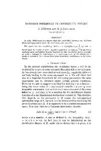
Fig. 1. images

The camera rig mounted on the robot used to obtain panoramic

Topological maps attempt to capture spatial connectivity of the environment by representing it as a graph with arcs connecting the nodes that designate significant places in the environment, such as corridor junctions and room entrances [27]. The arcs are usually annotated with navigation information. Arguably the hardest problem in robotic mapping is the perceptual aliasing problem, which is an instance of the data association problem, also variously known as “closing the loop” [17] or “the revisiting problem” [49]. It is the problem of determining whether sensor measurements taken at different points in time correspond to the same physical location. When a robot receives a new measurement, it has to decide whether to assign this measurement to one of the locations it has visited previously, or to a completely new location. The aliasing problem is hard as the number of possible choices grows combinatorially. Indeed, we demonstrate below that the number of choices is the same as the number of possible partitions of a set, which grows hyper-exponentially with the cardinality of the set. Previous solutions to the aliasing problem [52][24] commit to a specific correspondence between measurements and locations at each step, so that once a wrong decision has been made, the algorithm cannot recover. Other solutions [26][9][25] perform well in most situations but fail silently in environments where the problem is particularly hard, thus returning a wrong map of the environment. The major contribution of this work is the idea of defining a probability distribution over the space of topological maps

Fig. 2.

A panoramic image obtained from the robot camera rig

and the use of sampling in order to obtain this distribution. The key realization here is that a distribution over this combinatorially large space can be succinctly approximated by a sample set drawn from the distribution. In this paper, we describe Probabilistic Topological Maps (PTMs), a samplebased representation that captures the posterior distribution over all possible topological maps given the available sensor measurements. The intuitive reason for computing the posterior is to solve the aliasing problem for topologies in a systematic manner. The set of all possible correspondences between measurements and the physical locations from which the measurements are taken is exactly the set of all possible topologies. By inferring the posterior on this set, whereby each topology is assigned a probability, it is possible to locate the more probable topologies without committing to a specific correspondence at any point in time, thus providing the most general solution to the aliasing problem. Even in pathological environments, where almost all current algorithms fail, our technique provides a quantification of uncertainty by pegging a probability of correctness to each topology. While sample-based estimation of the posterior over data associations has previously been discussed in computer vision [5], its use in robotic mapping to find a distribution over all possible maps is completely novel to the best of our knowledge. As a second major contribution, we show how to perform inference in the space of topologies given uncertain sensor data from the robot. We provide a general theory for incorporating odometry and appearance measurements in the inference process. More specifically, we describe an algorithm that uses Markov chain Monte Carlo (MCMC) sampling [13] to extend the highly successful Bayesian probabilistic framework to the space of topologies. To enable sampling over topologies using MCMC, each topology is encoded as a set partition over the set of landmark measurements. We then sample over the space of set partitions, using as target distribution the posterior probability of the topology given the measurements. Another important aspect of this work is the definition of a simple but effective prior on the density of landmarks in the environment. We demonstrate that given this prior, the additional sensor information needed can be very scant indeed. In fact, our method is general and can deal with any type of sensor measurement or prior knowledge. Moreover, any newly available information from the sensors can be used to augment the previous available information to improve the quality of the PTM. In our experiments, we show that even when the system produces nice maps of the environment using only odometry measurements, we can get better quality maps by using appearance data in addition to the odometry.

We provide a general-purpose appearance model in this work and illustrate its application using Fourier signatures [20][32] of panoramic images. The panoramic images are obtained from a camera rig mounted on a robot as shown in Figure 1. An example of such a panoramic image is shown in Figure 2. Fourier signatures, which have previously been used in the context of memory-based navigation [32] and localization using omni-directional vision [33], are a lowdimensional representation of images using Fourier coefficients. They allow easy matching of images to determine correspondence. Further, due to the periodicity of panoramic images, Fourier signatures are rotation-invariant. This property is of prime importance when determining correspondence since the robot may be moving in different directions when the images are obtained. In subsequent sections, we provide related work in probabilistic mapping in general and topological mapping in particular. Then, we define Probabilistic Topological Maps formally and provide a theory for estimating the posterior over the space of topologies. Subsequently, we describe an implementation of the theory using MCMC sampling in topological space, followed by a section with details about the specific odometry and appearance models we used. A prior over the space of topologies is also described. Finally, in Section VII we provide experimental validation for our technique. II. R ELATED W ORK Our work relates to the area of probabilistic mapping and, more specifically, to topological mapping. Below we review relevant prior research in these areas. A. Probabilistic Mapping and SLAM Early approaches to the mapping problem (usually obtained by solving the SLAM problem) used Kalman filters and Extended Kalman filters [28][3][6][10][48][47] on landmarks and robot pose. Kalman filter approaches assume that the motion model, the perceptual model (or the measurement model) and the initial state distribution are all Gaussian distributions. Extended Kalman filters relax these assumptions by linearizing the motion model using a Taylor series expansion. Under these assumptions, the Kalman filter approach can estimate the complete posterior over maps efficiently. However, the Gaussian assumptions mean that it cannot maintain multimodal distributions induced by the measurement of a landmark that looks similar to another landmark in the environment. In other words, the Kalman filter approach is unable to cope with the correspondence problem. A well-known algorithm that incorporates smoothing, instead of Kalman filtering, is the Lu/Milios algorithm [30],

a laser-specific algorithm that performs maximum likelihood estimation of the correspondence. It iterates over a map estimation and a data association phase that enable it to recover from wrong correspondences in the presence of small errors. However, the algorithm encounters limitations when faced with large pose errors and fails in large environments. Rao-Blackwellized Particle Filters (RBPFs) [38], of which the FastSLAM algorithm [36] is a specific implementation, are also theoretically capable of maintaining the complete posterior distribution over maps under assumption of Gaussian measurements. This is possible since each sample in the RBPF can represent a different data association decision [35]. However, in practice the dimensionality of the trajectory space is too large to be adequately represented in this approach, and often the ground-truth trajectory along with the correct data association will be missed altogether. This problem is a fundamental shortcoming of the importance sampling scheme used in the RBPF, and cannot be dealt with satisfactorily except by an exponential increase in the number of samples, which is intractable. One solution to this problem, which involves keeping all possible data associations in a tree and searching through them at each time step, is given in [18]. Another problem with RBPFs is their sensitivity to odometry drift over time. Recent work by Haehnel et al. [17] tries to overcome the odometry drift by correcting for it through scan matching, but this only alleviates the problem without solving it completely. Yet another approach to SLAM that has been successful is the use of the EM algorithm to solve the correspondence problem in mapping [52][2]. The algorithm iterates between finding the most likely robot pose and the most likely map. EM-based algorithms do not compute the complete posterior over maps, but instead perform hill-climbing to find the most likely map. Such algorithms make multiple passes over sensor data which makes them extremely slow and unfit for on-line, incremental computation. In addition, EM cannot overcome local minima, resulting in incorrect data associations. Other approaches exist that report loop closures and re-distribute the error over the trajectory [16][39][51][49], but these decisions are again irrevocable and hence mistakes cannot be corrected. Recent work by Duckett [7] on the SLAM problem is similar to our own, in the sense that he too deals with the space of possible maps. The SLAM problem is presented as a global optimization problem and metric maps are coded as chromosomes for use in a genetic algorithm. The genetic algorithm searches over the space of maps (or chromosomes) and finds the most likely map using a fitness function. This approach differs from ours by computing the maximum likelihood solution as opposed to the complete posterior as we do. In consequence, it suffers from brittleness similar to other techniques described previously. B. Topological Maps Maintaining the posterior distribution over the space of topologies results in a systematic and robust solution to the aliasing problem that plagues robot mapping. Though probabilistic methods have been used in conjunction with

topological maps before, none exist that are capable of dealing with the inference of the posterior distribution over the space of topologies. A recent approach gives an algorithm to build a tree of all possible topological maps that conform to the measurements, but in a non-probabilistic manner [44][43]. Dudek. et. al. [8] have also given a technique that maintains multiple hypotheses regarding the topological structure of the environment in the form of an exploration tree. Most instances of previous work extant in the literature that incorporate uncertainty in topological map representations do not deal with general topological maps, but with the use of markov decision processes to learn a policy that the robot follows to navigate the environment. Simmons and Koenig [46] model the environment using a POMDP in which observations are used to update belief states. Another approach that is closer to the one presented here, in the sense of maintaining a multi-hypothesis space over correspondences, is given by Tomatis et al. [55] and also uses POMDPs to solve the correspondence problem. However, while in their case a multi-hypothesis space is maintained, it is used only to detect the points where the probability mass splits into two. Also, like a lot of others, this work uses specific qualities of the indoor environment such as doors and corridor junctions, and hence is not generally applicable to any environment. Shatkay and Kaelbling [45] use the Baum-Welch algorithm, a variant of the EM algorithm used in the context of HMMs, to solve the aliasing problem for topological mapping. Other examples of HMM-based work include [23][15] and [1] where a second order HMM is used to model the environment. Lisien et al. [29] have provided a method that combines locally estimated feature-based maps with a global topological map. Data association for the local maps is performed using a simple heuristic wherein each measurement is associated with the existing landmark having the minimum distance to the measured location. A new landmark is created if this distance is above a threshold. The set of local maps is then combined using an “edge-map” association, i.e. the individual landmarks are aligned and the edges compared. This technique, while suitable for mapping environments where the landmark locations are sufficiently dissimilar, is not robust in environments with large or multiple loops. Many topological approaches to mapping, related to our work only in the sense that they form a significant part of the topological mapping literature, include robot control to help solve the correspondence problem. This is achieved by maneuvering the robot to the exact spot it was in when visiting the location previously, so that correspondence becomes easier to compute. Examples of this approach include Choset’s Generalized Voronoi Graphs [4] and Kuipers’ Spatial Semantic Hierarchy [27]. Other approaches that involve behaviorbased control for exploration-based topological mapping are also fairly common. Mataric [31] uses boundary-following and goal-directed navigation behaviors in combination with qualitative landmark identification to find a topological map of the environment. A complete behavior-based learning system based on the Spatial Semantic Hierarchy that learns at many levels starting from low-level sensori-motor control to topological and metric maps is described in [41]. Yamauchi

et al. [56][57] use a reactive controller in conjunction with an Adaptive Place Network that detects and identifies special places in the environment. These locations are subsequently placed in a network denoting spatial adjacency. Some other approaches use a non-probabilistic approach to the correspondence problem by applying a clustering algorithm to the measurements to identify distinctive places, an instance being [26]. Finally, SLAM algorithms used to generate metric maps have also been applied to generating integrated metric and topological maps with some success. For instance, Thrun et al. [53] use the EM algorithm to solve the correspondence problem while building a topological map. The computed correspondence is subsequently used in constructing a metric map. By contrast, Thrun [50] first computes a metric map using value iteration and uses thresholding and Voronoi diagrams to extract the topology from this map. III. P ROBABILISTIC T OPOLOGICAL M APS A Probabilistic Topological Map is a sample-based representation that approximates the posterior distribution P (T |Z) over topologies T given observations Z. While the space of possible maps is combinatorial, a probability density over this space can be approximated by drawing a sample of possible maps from the distribution. Using the samples, it is possible to construct a histogram on the support of this sample set. We do not consider the issue of landmark detection in this work. Instead, we assume the availability of a “landmark detector” that simply detects a landmark when the robot is near (or on) a landmark. Subsequently, odometry and appearance measurements from the landmark location are stored, the appearance measurements being in the form of images. The odometry can be said to measure the landmark location while the images measure the landmark appearance. No knowledge of the correspondence between landmark measurements and the actual landmarks is given to the robot: indeed, that is exactly the topology that we seek. The problem then is to compute the discrete posterior probability distribution P (T |Z) over the space of topologies. Our technique exploits the equivalence between topologies of an environment and set partitions of landmark measurements, which group the measurements into a set of equivalence classes. When all the measurements of the same landmark are grouped together, this naturally defines a partition on the set of measurements. It can be seen that a topology is nothing but the assignment of measurements to sets in the partition, resulting in the above mentioned isomorphism between topologies and set partitions. An example of the encoding of topologies as set partitions is shown in Figure 3. We begin our consideration by assuming that the robot observes N “special places” or landmarks during a run, not all of them necessarily distinct. The number of distinct landmarks in the environment, which is unknown, is denoted by M . Formally, for the N element measurement set Z = {Zi |1 ≤ i ≤ N }, a partition T can be represented as T = {Sj | j ∈ [1, M ]}, where each Sj is a set of measurements such that SM Sj1 ∩ Sj2 = φ ∀j1, j2 ∈ [1, M ], j1 6= j2, j=1 Sj = Z, and M ≤ N is the number of sets in the partition. In the context

4

3

3 4 2 2

5

0

1

0

1

(a)

(b)

Fig. 3. Two topologies with 6 observations each corresponding to set partitions (a) with six landmarks ({0}, {1}, {2}, {3}, {4}, {5}) and (b) with five landmarks({0}, {1, 5}, {2}, {3}, {4}) where the second and sixth measurement are from the same landmark.

of topological mapping, all members of the set Sj represent landmark observations of the jth landmark. The cardinality of the set of all possible topologies is identical to the number of set partitions of the observation N -set. This number is P∞ N called the Bell number bN [40], defined as bN = 1e k=0 kk! , and grows hyper-exponentially with N , for example b2 = 2, b3 = 5 but b15 =1382958545. The combinatorial nature of this space makes exhaustive evaluation impossible for all but trivial environments. IV. A G ENERAL F RAMEWORK

FOR I NFERRING

PTM S

The aim of inference in the space of topologies is to obtain the posterior probability distribution on topologies P (T |Z). All inference procedures that compute sample-based representations of distributions require that evaluation of the sampled distribution be possible. In this section, we describe the general theory for evaluating the posterior at any given topology. Using Bayes Law on the posterior P (T |Z), we obtain P (T |Z) ∝ P (Z|T )P (T )

(1)

where P (T ) is a prior on topologies and P (Z|T ) is the observation likelihood. In this work, we assume that the only observations we possess are odometry and appearance. Note that this is not a limitation of the framework, and other sensor measurements, such as laser range scans, can easily be taken into consideration. We factor the set Z as Z = {O, A} , where O and A correspond to the set of odometry and appearance measurements respectively. This allows us to rewrite (1) as P (T | O, A)

= kP (O, A|T )P (T ) = kP (O|T )P (A|T )P (T )

(2)

where k is the normalization constant, and we have assumed that the appearance and odometry are conditionally independent given the topology. We discuss evaluation of the appearance likelihood P (A|T ), odometry likelihood P (O|T ), and the prior on topologies P (T ), in the following sections. A. Evaluating the Odometry Likelihood It is not possible to evaluate the odometry likelihood P (O|T ) without knowledge of the landmark locations. However, since we are do not require the landmark locations when

be factored into a product of likelihoods of the individual appearance instances. This is illustrated using an example topology in Figure 4, where the Bayesian network encodes the independence assumptions in the appearance measurements. Hence, denoting the jth set in the partition as Sj , we rewrite P (A | Y, T ) as P (A | Y, T ) =

M Y Y

P (ai | yj )

(6)

j=1 ai ∈Sj

Fig. 4. The Bayesian network (b) that encodes the independence assumptions for the appearance measurements in the topology (a) given the true appearance Y = {y1 , . . . , y5 } at all the landmark locations. The measurements corresponding to different landmarks are independent.

inferring topologies, we integrate over the set of landmark locations X and calculate the marginal distribution P (O|T ): Z P (O|T ) = P (O|X, T )P (X|T ) (3) X

where P (O|X, T ) is the measurement model, a probability density on O given X and T , and P (X|T ) is a prior over landmark locations. Note that (3) makes no assumptions about the actual form of X, and hence, is completely general. Evaluation of the odometry likelihood using (3) requires the specification of a prior distribution P (X|T ) over landmark locations in the environment and a measurement model P (O|X, T ) for the odometry given the landmark locations. B. Evaluating the Appearance Likelihood Similar to the case of the odometry likelihood, estimation of the appearance likelihood P (A | T ), where A = {ai |1 ≤ i ≤ N } is the set of appearance measurements, is performed by introducing the hidden parameter Y = {yj |1 ≤ j ≤ M }. This hidden parameter denotes the “true appearance” corresponding to each landmark in the topology. As we do not need to compute Y when inferring topologies, we marginalize over it so that Z P (A | T ) = P (A | Y, T )P (Y | T ) (4) Y

where P (A|Y, T ) is the measurement model and P (Y | T ) is the prior on the appearance. We assume that the appearance of a landmark is independent of all other landmarks, so that each yj is independent of all other yj 0 . The prior P (Y | T ) can thus be factored into a product of priors on the individual yj . M Y P (Y | T ) = P (yj ) (5)

where the dependence on T is subsumed in the partition. Combining Equations (4), (5) and (6), we get the expression for the appearance likelihood as M Z Y Y P (ai | yj ) (7) P (yj ) P (A | T ) = j=1

yj

ai ∈Sj

In the above equation, P (yj ) is a prior on appearance in the environment, and P (ai | yj ) is the appearance measurement model. Evaluation of the appearance likelihood requires the specification of these two quantities. C. Prior on Topologies The prior on topologies P (T ), required to evaluate (2), assigns a probability to topology T based on the number of distinct landmarks in T and the total number of measurements. The prior is obtained through the use of the Classical Occupancy Distribution [21]. In the interest of continuity, the derivation of the prior is deferred to Appendix A. We simply state the expression for the prior, given the total number of landmarks in the environment L (including those not visited by the robot) L−N × L! P (T |L) = k (8) (L − M )! where N is the number of measurements, M is the number of distinct landmarks in the topology T , and k is a normalization constant. This prior distribution assigns equal probability to all topologies containing the same number of landmarks. Note that the total number of landmarks in the environment, L, is not known. Hence, we assume a Poisson prior on L, L −λ e giving P (L|λ) = λ L! , and marginalize over L to get the actual prior on topologies X P (T ) = P (T |L)P (L|λ) L

∝ e−λ

∞ X L−N × λL (L − M )!

(9)

L=M

where λ is the Poisson parameter and the summation replaces the integral as the Poisson distribution is discrete. In practice, the prior on L is a truncated Poisson distribution since the summation in (9) is only evaluated for a finite number of terms.

j=1

The topology T introduces a partition on the set of appearance measurements by determining which “true appearance” yj each measurement ai actually measures, i.e the partition encodes the correspondence between the set A and the set Y . Also, given Y , the likelihood of the appearance can

V. I NFERRING P ROBABILISTIC T OPOLOGICAL M APS USING MCMC The previous section provided a general theory for inferring the posterior over topologies using odometry and appearance information. We now present a concrete implementation of the

Fig. 5. An example of a PTM giving the most probable topologies in the posterior distribution obtained using MCMC sampling. The histogram gives the probability of each topology.

Algorithm 1 The Metropolis-Hastings algorithm 1) Start with a valid initial topology Tt , then iterate once for each desired sample 0 2) Propose a new topology Tt using the proposal distribution 0 Q(Tt ; Tt ) 3) Calculate the acceptance ratio a=

P (Tt0 |Z t ) Q(Tt ; Tt0 ) P (Tt |Z t ) Q(Tt0 ; Tt )

(10)

where Z t is the set of measurements observed up to and including time t. 4) With probability p = min(1, a), accept Tt0 and set Tt ← Tt0 . If rejected we keep the state unchanged (i.e. return Tt as a sample).

theory that uses the Metropolis-Hastings algorithm [19], a very general MCMC method, for performing the inference. Figure 5 depicts an example of the discrete posterior over topologies obtained using our MCMC-based technique. All MCMC methods work by running a Markov chain over the state space with the property that the chain ultimately converges to the target distribution of our interest. Once the chain has converged, subsequent states visited by the chain are considered to be samples from the target distribution. The Markov chain itself is generated using a proposal distribution that is used to propose the next state in the chain, a move in state space, possibly by conditioning on the current state. The Metropolis-Hastings algorithm provides a technique whereby the Markov chain can converge to the target distribution using any arbitrary proposal distribution, the only important restriction being that the chain be capable of reaching all the states in the state space. The pseudo-code to generate a sequence of samples from the posterior distribution P (T |Z) over topologies T using the Metropolis-Hastings algorithm is shown in Algorithm 1 (adapted from [13]). In this case the state space is the space of all set partitions, where each set partition represents a different topology of the environment. Intuitively, the algorithm samples from the desired probability distribution P (T |Z) by rejecting a fraction of the moves generated by a proposal distribution Q(Tt0 ; Tt ), where Tt is the current state and Tt0 is the proposed state. The fraction of moves rejected is governed by the acceptance ratio a given by (10), which is where most of the computation takes place. Computing the acceptance ratio, and hence, sampling using MCMC, requires the design of a proposal density and evaluation of the target density, the details of which are discussed below.

Fig. 6. Illustration of the proposal - Given a topology (a) corresponding to the set partition with N =5, M =4, the proposal distribution can (b) perform a merge step to propose a topology with a smaller number of landmarks corresponding to a set partition with N =5, M =3 or (c) perform a split step to propose a topology with a greater number of landmarks corresponding to a set partition with N =M =5 or re-propose the same topology.

We use a simple split-merge proposal distribution that operates by proposing one of two moves, a split or a merge with equal probability at each step. Given that the current sample topology has M distinct landmarks, the next sample is obtained by splitting a set, to obtain a topology with M + 1 landmarks, or merging two sets, to obtain a topology with M − 1 landmarks. The proposal is illustrated in Figure 6 for a trivial environment. If the chosen move is not possible, the current topology is re-proposed. An example of an impossible move is a merge move on a topology containing only one landmark. The merge move merges two randomly selected sets in the partition to produce a new partition with one less set than before. The probability of a merge is simply 1/NM where NM is the number of
possible merges and is equal to the binomial coefficient M 2 , (M > 1). The split move splits a randomly selected set in the partition to produce a new partition with one more set than before. To calculate the probability of a split move, let NS be the number of non-singleton sets in the partition. Clearly, NS is the number of sets in the partition that can be split. Out of these NS sets, we pick a random set R to split. The number |R| of possible  n ways to split R into two subsets is given by 2 , where m denotes the Stirling number of the second kind that gives the number of possible ways to split a set of size n  n ∆  n−1 into m subsets, and is defined recursively as m = m−1 + n−1 m m [40]. Combining the probability of selecting R and the probability of splitting obtain the probability of the  it, we −1 |R| split move as psplit = NS 2 . The proposal distribution is summarized in pseudo-code format in Algorithm 2, where Q is the proposal distribution 0 →T ) is the proposal ratio, a part of the acceptance and r = q(T q(T →T 0 ) ratio in Algorithm 1. Note that this proposal does not incorpo-

Algorithm 2 The Proposal Distribution 1) Select a merge or a split with probability 0.5 2) Merge move: 0 • if T contains only one set, re-propose T = T , hence r=1 • otherwise select two sets at random, say R and S a) T 0 = (T − {R} − {S})∪{R∪S} and Q(T → T 0 ) = 1 NM

b) Q(T 0 → T ) is obtained from the reverse case 3(b), −1 , where NS is the hence r = NM NS
|R 2 S|  number of possible splits in T 0 3) Split move: 0 • if T contains only singleton sets, re-propose T = T , hence r = 1 • otherwise select a non-singleton set U at random from T and split it into two sets R and S. a) T 0 = (T − {U }) ∪ {R, S} and Q(T → T 0 ) = −1

NS
|U2 |   b) Q(T 0 → T ) is obtained from the reverse case 2(b), −1 hence r = NM NS
|U2 |  , where NM is the number of possible merges in T 0

rate any domain knowledge, but uses only the combinatorial properties of set partitions to propose random moves. In addition to proposing new moves in the space of topologies, we also need to evaluate the posterior probability P (T |Z). This is done as described in Section IV. The specification of the measurement models and the details of evaluating the posterior probability using these models are given in the following section. VI. E VALUATING THE P OSTERIOR D ISTRIBUTION We evaluate the posterior distribution, which is also the MCMC target distribution, using the factored Bayes rule (2). It is important to note that we do not need to calculate the normalization constant in (2) since the Metropolis-Hastings algorithm requires only a ratio of the target distribution evaluated at two points, wherein the normalization constant cancels out. The odometry and appearance measurement models required to evaluate (2) are described below. A. Evaluating the Odometry Likelihood Evaluation of the odometry likelihood is performed using (3) Z P (O|T ) = P (O|X, T )P (X|T ) X

under the assumption, common in robotics literature, that landmark locations and odometry measurements have the 2D form X = {li = (xi , yi )|1 ≤ i ≤ N } and O = {ok = (xk , yk , θk )|1 ≤ k ≤ N − 1} respectively. This requires the definition of a prior on the distribution of the landmark locations X conditioned on the topology T , P (X|T ). We use a simple prior on landmarks that encodes our assumption that landmarks do not exist close together in the environment. If the topology T places two distinct landmarks li1 and li2 within a distance d of each other, the negative log

Fig. 7. Cubic penalty function (in this case, with a threshold distance of 3 meters) used in the prior over landmark density

Fig. 8. Illustration of optimization of the odometry likelihood. The observed odometry in (a) is transformed to the one in (b) because the topology used in this case, ({0, 4}, {1}, {2}, {3}) , tries to place the first and last landmarks at the same physical location.

likelihood corresponding to the two landmarks is given by the penalty function  f (d) d