of a simple and robust Bayesian intent inference approach that models the .... object reaches the a priori unknown intended destination D is denoted by T. Whilst ...
SUBMITTED TO IEEE TRANSACTIONS ON CYBERNETICS, VOL. XX, NO. XX, XXXX XXXX
1
Bayesian Intent Prediction in Object Tracking Using Bridging Distributions
arXiv:1508.06115v3 [stat.AP] 4 Feb 2016
Bashar I. Ahmad† , James K. Murphy† , Patrick M. Langdon and Simon J. Godsill
Abstract—In several application areas, such as human computer interaction, surveillance and defence, determining the intent of a tracked object enables systems to aid the user/operator and facilitate effective, possibly automated, decision making. In this paper, we propose a probabilistic inference approach that permits the prediction, well in advance, of the intended destination of a tracked object and its future trajectory. Within the framework introduced here, the observed partial track of the object is modeled as being part of a Markov bridge terminating at its destination, since the target path, albeit random, must end at the intended endpoint. This captures the underlying long term dependencies in the trajectory, as dictated by the object intent. By determining the likelihood of the partial track being drawn from a particular constructed bridge, the probability of each of a number of possible destinations is evaluated. These bridges can also be employed to produce refined estimates of the latent system state (e.g. object position, velocity, etc.), predict its future values (up until reaching the designated endpoint) and estimate the time of arrival. This is shown to lead to a low complexity Kalman-filter-based implementation of the inference routine, where any linear Gaussian motion model, including the destination reverting ones, can be applied. Free hand pointing gestures data collected in an instrumented vehicle and synthetic trajectories of a vessel heading towards multiple possible harbours are utilised to demonstrate the effectiveness of the proposed approach. Index Terms—Bayesian inference, Kalman filtering, tracking, maritime surveillance, Human computer interactions.
I. I NTRODUCTION
I
N several application areas such as surveillance, defence and human computer interaction (HCI), the trajectory of a tracked object, e.g. a vessel, jet, pedestrian or pointing apparatus, is driven by its final destination. Thus, a priori knowledge of the object endpoint can not only offer vital information on intent, unveil potential conflict or threat and enable task facilitation strategies, but can also produce more accurate tracking routines [1]–[9]. In this paper, we address the problem of predicting the intended destination of a tracked object from a finite set of possible endpoints and the future values of its hidden state (e.g. position, velocity, etc.), given the available noisy observations. This can be viewed as a means to assist or automate timely decision making, planning and resources allocation at a higher system level, compared with a conventional sensor-level tracker. The latter typically focuses on inferring the current value of the latent state Xt , with several well-established algorithms [10]–[12]. B. I. Ahmad*, J. K. Murphy, P. M. Langdon, S. J. Godsill are with the Engineering Department, University of Cambridge, Trumpington Street, Cambridge, UK, CB2 1PZ. Emails:{bia23, jm362, pml24, sjg30}@cam.ac.uk. † The first two authors made an equal contribution to this work.
To motivate the work presented here, consider the following two examples: 1) Maritime Surveillance: analysing the route and determining the destination of vessels in a given geographical area is necessary for maintaining maritime situational awareness (MSA), critical for maritime safety. This permits identification of potential threats, opportunities or malicious behaviour, allowing the protection of assets or other reactive actions [1], [2], [8], [9]. Given the complex nature of typical maritime traffic as well as the vast amounts of available information on tracked targets, there is a growing interest in increasing the degree of automation in MSA systems by unveiling the intent of object(s) of interest from available low level tracking data. Thus, there is a notable demand for low-complexity and reliable destination and trajectory prediction techniques. Similar challenges can be found in aerospace surveillance, with aircraft in lieu of vessels. 2) Interacting with touchscreen: touchscreens are becoming an integrated part of modern vehicles due to their ability to present large quantities of in-vehicle infotainment system data and offering additional design flexibility through a combined display-input-feedback module [13], [14]. Using these displays entails undertaking a free hand pointing gesture and dedicating a considerable amount of attention that would otherwise be available for driving. Hence, such interactions can act as a distractor from the primary task of driving and have safety implications [15]. The early inference of the intended onscreen item of the free hand pointing gesture can simplify and expedite the selection task, thus significantly improving the usability of in-vehicle touchscreens by reducing distractions (see [16] for an overview of the intent-aware display concept). There is a wide range of other applications that can benefit from knowing the intent of a target of interest. For example, predicting the destination of an intruder in a perimeter, inferring the future position of a moving person in a given area to take appropriate robotic actions [17], and advanced driver assistance system in vehicles [18], to name a few. A. Contributions The main contribution of this paper is the development of a simple and robust Bayesian intent inference approach that models the available partial trajectory of a tracked object as a random bridge terminating at a nominal destination. It can employ any linear Gaussian motion model, including Linear Destination Reverting (LDR) models, such as those detailed in Sections III-A and III-B, which are intrinsically driven by the endpoint of the tracked object (they were used
SUBMITTED TO IEEE TRANSACTIONS ON CYBERNETICS, VOL. XX, NO. XX, XXXX XXXX
in [16]). The bridging framework introduced here capitalises on the premise that the path of the object, albeit random, must end at the intended destination. Since the endpoint is unknown a priori, a bridge for each possible destination is constructed. This encapsulates the long term dependencies in the object trajectory due to premeditated actions guided by intent. By determining the likelihood of the observed partial track being drawn from a particular bridge, the probability of each nominal endpoint, along with a refined estimate of the current object state Xt and its future values Xs (for s > t), can be evaluated. This is accomplished via Kalman-filter-based inference, amenable to parallelisation. Notably, the proposed approach in this paper does not impose prior knowledge of the arrival time T at the intended destination D. A conservatively chosen prior distribution of the possible times of arrival for each destination suffices. This allows the introduction of a technique to sequentially estimate the posterior distribution p(T |D) of the arrival time T from the available partial trajectory of the tracked object. Within the formulation adopted here, possible destinations may also be specified as (Gaussian) distributions, with a mean and covariance, in order to model endpoints with a non-zero spatial extent; point destinations can be modelled by setting the covariance to zero. Finally, we conduct simulations to illustrate the inference capability of the bridging-distributionbased predictors using real pointing data (HCI) and synthetic vessel tracks (MSA). B. Related Work One of the first techniques to incorporate predictive information on the target endpoint to improve the accuracy of the tracking results was proposed in [1] and motivated various subsequent studies such as [3]. It assumes prior knowledge of the time of arrival at destination to devise a destination-aware tracker. In this paper, the objective is to predict the intended destination of the tracked object, using motion models that are also inherently dependent on the endpoint. This can be inferred using a multiple Kalman-filter-based solution, even without imposing knowledge of T . It is noted that unlike the widely used interacting multiple models (IMM) [11], [19] and generalised pseudo-Bayesian [20] approaches for manoeuvering targets, here we construct a bridge model per nominal destination and no interaction or switching among models is applied. This is based on the premise that the tracked object intent is set well in advance of reaching its endpoint, leading to simple and low complexity algorithms. More recently, destination-aware trackers that facilitate inference of the object state Xt followed by an additional mechanism to determine its endpoint are presented in [5]–[7], succeeding the work in [21]. The object trajectory is modelled as a discrete stochastic reciprocal or context-free grammar process, which can be regarded as non-causal generalisations of Markov processes. The state space is discretised within predefined regions, for example, the spatial dimensions are divided into finite grids. The target can accordingly pass through a finite number of zones. Here, in contrast, we adopt continuous state space models with bridging distributions
2
that do not impose any discretisation/restrictions on the path the tracked object has to follow to reach its endpoint. This formulation is particularly important in applications where discretisation of the spatial area is burdensome, e.g. tracking objects in 3D as with free hand pointing gestures or surveying a large geographical area for MSA. The method proposed here provides a simple, effective solution to the intent prediction problem compared with those in [6], [7]; it also combines the destination prediction and tracking operations. Intent inference is often treated within the context of anomaly detection, e.g. [2], [4], [6]–[9], [22]. A common approach is to categorise each trajectory of the tracked object(s) as either normal or anomalous, i.e. classification techniques. This follows defining (or learning from recorded data) a pattern of life that constitutes ordinary behaviour. Deviations from this are considered to indicate an anomaly, assuming adequate data association algorithms [2], [8]. For example, a support vector machine (SVM) based method is introduced in [5] to classify deviant trajectories. A model-based technique, based on a tuned hidden Markov model, is utilised in [9] to characterise a pattern of life and predict the future position of a conforming target. Similarly, in [6] and related work, ‘tracklets’, which are sub-patterns comprising a trajectory, are defined as a means to capture a semantic interpretation of complex patterns such as anomaly or intent. In this paper, a probabilistic modelbased formulation is proposed to tackle the intent inference problem rather than anomaly detection, with the posterior probabilities of various intents sequentially calculated using bridging distributions. The benefits of predicting the intended item on a Graphical User Interface (GUI) early in a pointing task are widely recognised in HCI, e.g. [23]–[26]. Most existing algorithms focus on pointing via a mechanical device, such as a mouse, in a 2D setup. In [16], 2D–based predictors are shown to be unsuitable for pointing tasks in 3D. For instance, the linear-regression methods in [24] and [25] assume that the the destination is always located along the path followed by the pointing object, which is rarely true in free hand pointing gestures. Endpoint inference based on modelling the pointing movements as a linear destination reverting process is considered in [16]. Compared to [16], the bridging-based-solution developed here is more general and more robust to variability in the target behaviour, leading to superior prediction results. Finally, data driven prediction/classification techniques, such as in [17], [18], [26], [27], rely on a dynamical model learnt from recorded tracks/behaviour. This often entails a high computational cost and necessitates substantial parameters training from complete data sets (not always available). In this paper, as is common in tracking applications [10]–[12], known dynamical and sensor models (e.g. due to practical physical constraints), albeit with unknown parameters, are presumed, i.e. a state-space-modelling approach. It requires minimal training, is amenable to parallelisation and is computationally efficient, yet delivers a competitive performance. C. Paper Outline The remainder of this paper is organised as follows. In Section II, we formulate the tackled problem and objectives. A
SUBMITTED TO IEEE TRANSACTIONS ON CYBERNETICS, VOL. XX, NO. XX, XXXX XXXX
3
range of possible motion models are outlined in Section III and the prior of the state value at destination, i.e. XT , is addressed. In Section IV, the bridging-based-prediction is introduced and pseudo-code for the proposed algorithms is provided. The performance of the proposed techniques is evaluated in Section V using real free hand pointing gesture data and synthetic vessel tracks. Finally, conclusions are drawn in Section VI.
with εt ∼ N (0, Q(h, d)). The matrices F and Q as well as the vector M , which together define the state transition from one time to another, are functions of the time step h and the destination d. The nth observation yn is modelled as a linear function of the time tn state perturbed by additive Gaussian noise,
II. P ROBLEM S TATEMENT Let D = {d : d = 1, ..., N } be the set of N nominal destinations, e.g. harbours where a vessel can dock or selectable icons displayed on a touchscreen. The time instant the tracked object reaches the a priori unknown intended destination D is denoted by T . Whilst no assumptions are made about the layout of D, each endpoint is modelled as an extended region, e.g. GUI icons or harbour, rather than a single point as in [16]. Hence, the dth destination is defined by the (Gaussian) distribution d v N (ad , Σd ); see Section III-C. The objective here is to dynamically determine the probability of each possible endpoint being the intended destination,
where νn ∼ N (0, Vn ). No assumption is made about the observation arrival times tn and irregularly spaces, asynchronous observations can naturally be incorporated within the framework presented here. Based on (3) and (4), a Kalman filter can be utilised to calculate both the posterior distribution of the latent state and the observation likelihood for the current set of measurements y1:n [28], conditioned on knowing d. The computationally efficient Kalman filter is particularly desirable since running, concurrently, multiple Kalman filters for d ∈ D, in real-time, is plausible, even in settings where limited computing power is available, such as on a vehicle touchscreen or a portable battery-powered system. To condition on the destination, the inference framework requires that the transition density of such models can be calculated both from one observation to the next (i.e. from time instant tn−1 to tn ) and from the current observation time to the arrival time at the intended endpoint (i.e. from tn to T ). Continuous-time motion models are therefore a natural choice, where the tracked object dynamics is represented by a continuous-time stochastic differential equation (SDE). This SDE can be integrated to obtain a transition density over any time interval. For Gaussian linear time invariant (LTI) models, this integration is analytically tractable, giving transition functions of the form in (3). This class of models includes many widely used ones, e.g. (near) constant velocity (CV) and (near) constant acceleration (CA) models, as well as the linear destination reverting models given below. The early work in [16] employs LDR models in a forward sense, without using the destination state as conditioning information. In this paper, by contrast, a prior probability distribution on the object state at its destination XT is used directly as conditioning information in the inference procedure. This is achieved by using bridging distributions to introduce the longer term dependencies in the target trajectory (see Section III-C). A similar idea is explored in the preliminary study in [29] using the CV model, in which the endpoint information does not feature in the motion model. That work also specifies each destination as a single point (rather than a prior distribution) and applies a two step modified Kalman filter to infer D, which is more computationally demanding and obscure compared with the solution presented here. In the remainder of this section, we describe the LDR models of [16] for completion, other related motion processes and the prior of XT . The predictive position and velocity distributions of selected motion models, with and without the use of bridging (i.e. conditioning on XT ) are depicted in Figure 1 in the one dimensional case. The figure demonstrates the substantial effect of introducing the bridging assumptions on the prediction results of various motion models. It clearly shows how these distributions more accurately model the
P(tn ) = {p(D = d | y1:n ) : d = 1, 2, ..., N }
(1)
where y1:n , {y1 , y2 , ..., yn } is the available partial trajectory or observations of the tracked object at the time instant tn 6 T . 0 For example, as in [16], we have yk = [ˆ xtk yˆtk zˆtk ] is the Cartesian coordinates of the pointing finger at tk as captured by the pointing-gesture tracking device. Each observation is assumed to be derived from a true, but unknown, underlying target state Xtn at time tn , which can include position, velocity and higher order kinematics. Given P(tn ), the Maximum a Posteriori (MAP) estimate ˆ n ) = arg max p(D = d | y1:n ), D(t
(2)
d=1,2,...,N
is an intuitive approach to determine the intended endpoint D following the arrival of the new observation yn . It should be noted that other decision criteria can be adopted, although this is not treated here. Therefore, the proposed probabilistic endpoint prediction relies on a belief-based inference, i.e. calculating P(tn ) in (1), followed by a classifier, e.g. (2). As well as establishing D at time tn , a refined estimate of the system latent state Xtn and its predicted future values, i.e. Xt∗ for t∗ > tn , and time of arrival at D are sought. A successful prediction at tn of the tracked object’s final destination and/or its future trajectory can reveal its intention, alerting an operator T −tn in advance of any potential conflict or reducing the pointing time by T − tn in an HCI context. III. S YSTEM M ODELS A linear and Gaussian motion model for the evolution of the physical state Xt of the tracked object is assumed throughout this paper. Whilst the system governing the target dynamics does not change over time, it does depend on the object eventually reaching its destination D ∈ D. Conditioned on knowing the endpoint D = d, this leads to a linear timeinvariant Gaussian system such that the relationship between the system state at times t and t + h can be written as Xt+h = F (h, d)Xt + M (h, d) + εt
(3)
yn = GXtn + νn
(4)
SUBMITTED TO IEEE TRANSACTIONS ON CYBERNETICS, VOL. XX, NO. XX, XXXX XXXX
4
Weiner process. The diagonal structure of σ implies that the noise is independent in each spatial dimension, which is a common assumption in tracking [10]. However, this can be relaxed as shown in equation (7) below. As in [16], by integrating (5) from t to t + h, we obtain a state transition function in the form of equation (3) with FMRD (h, d) = e−Λh , MMRD (h, d) = (Is − e−Λh )pd , (6) � 1� Is − e−2Λh Λ−1 σ 2 , QMRD (h, d) = 2 where Is is the s × s identity matrix. For non-diagonal σ, the (i, j)th element of QMRD is given by i (σσ 0 )ij h (7) 1 − e−(Λii +Λjj )h , QMRD,ij = Λii + Λjj where z 0 is the transpose of the vector/matrix z. A special case of the MRD model occurs when Λ = 0s (with 0s being the s × s matrix of zeros), in which case the dynamics of the target position follow a Brownian motion (BM). In this case, the F , M and Q matrices in (3) become FBM (h, d) = hIs , MBM (h, d) = 0s×1 , Figure 1: Predictive distribution at t = 0 of position without bridging (first column), predictive position with bridging (second column), and predictive velocity with bridging (third column) for the BM, MRD, CV and ERV models in 1D. The x-axis shows time t and yaxis depicts position/velocity. The destination (black star), is located at position 10 at time T = 10. Grey shading shows one standard deviation, white line depicts the mean (except for BM and MRD velocity, for which the black line shows the implied mean of velocity only). Parameters for the models are σ = 1 (all models), λ = 0.3 (MRD), η = 0.1, ρ = 0.5 (ERV).
predicted state at the endpoint. It is worth noting that any continuous-time LTI model could be used directly within the proposed inference framework, as long as the system can be expressed by equations (3) and (4). A. Mean Reverting Diffusion (MRD) The position of the tracked object for the Mean Reverting Diffusion (MRD) model follows an Ornstein-Uhlenbeck process [30], with its mean being the destination. The intuition behind MRD is that a target heading towards a particular endpoint will revert towards it. The reversion strength is stronger the further the target is from its destination. This produces the predictive position and velocity dynamics of the form displayed in the second row of Figure 1. The state Xt of the mean reverting diffusion model consists of only the target position in each of the s spatial dimensions. For endpoint d (located at position pd ), the SDE is given by
(8)
2
QBM (h, d) = hσ , where 0s×1 is an s × 1 column vector of zeros. If measurements yn are direct noisy observations of the tracked object position, the observation matrix G in equation (4) is simply the identity matrix, G = Is . B. Equilibrium Reverting Velocity (ERV) In the ERV model, introduced in [16] for tracking and destination inference for pointing tasks on in-car displays, the system state Xt at time t is a 2s × 1 vector, arranged as [x1 , ..., xs , x˙ 1 , ..., x˙ s ]0 , where xi is the position in spatial dimension i, and x˙ i is the velocity in that dimension. Under this model, the SDE governing the evolution of the tracked object state is dXt = A (µd − Xt ) dt + σdwt ,
(9)
(5)
where the mean µd = [p0d , 00s×1 ]0 contains the position pd of destination d; wt is a standard s dimensional Wiener process and B = [0s , σ] is a 2s×s matrix that controls the noise which affects the velocity components of the process (modelling random forces acting on the target). In this case, σ can be given by the s × s Cholesky decomposition of the velocity noise covariance Σ, such that Σ = σσ 0 . As with the MRD model, a common choice is a diagonal σ, i.e. independent noise in each spatial dimension. The matrix A is given by � � 0 −Is A= s , η ρ
where Λ is a diagonal matrix with diagonal elements {λi }si=1 that set the reversion coefficient in each dimension. The diagonal matrix σ specifies the standard deviation of the dynamic noise and wt is a standard (unit variance) s-dimensional
where ρ is an s × s diagonal matrix of the drag coefficients (can be assumed to be the same across all dimensions) and η is a s × s diagonal matrix of the mean reversion strengths in each spatial dimension.
dXt = Λ (pd − Xt ) dt + σdwt ,
SUBMITTED TO IEEE TRANSACTIONS ON CYBERNETICS, VOL. XX, NO. XX, XXXX XXXX
A physical interpretation of the ERV model is that the destination d exerts an attractive force on the tracked object, of strength proportional to the distance separating them. This can be viewed as a linear spring of zero natural length connecting the target to its endpoint. A drag term proportional to the velocity of the target is also included, allowing the velocity profile of the tracked object (e.g. pointing-finger-tip in a free hand pointing gesture) to be correctly modelled; see Figure 1 (fourth row) and [16]. Integrating the SDE in (9) from t to t + h allows the system evolution to be expressed in the form in equation (3) with FERV (h, d) = e−Ah , MERV (h, d) = (I2s − e−Ah )µd , (10) Z t+h 0 QERV (h, d) = e−A(t+h−v) σσ 0 e−A (t+h−v) dv. t
The covariance matrix QERV (h, d) can be calculated by Matrix Fraction Decomposition [31] where QERV (h, d) = JK −1 , � � �� J −A = exp K 02s
� �� � σσ 0 02s h . A0 I2s
A special case of the ERV model occurs when η and ρ are both zero. In this scenario, the model reduces to the widely used (near) constant velocity model with � � I hIs FCV (h, d) = s , 0s Is MCV (h, d) = 02s×1 , " 3 σσ 0 h3 QCV (h, d) = 2 σσ 0 h2
(11) 2 σσ 0 h2 0
σσ h
# .
object velocity at the destination. If this is unknown, a large prior variance can be used to model this uncertainty. IV. I NTENT I NFERENCE U SING B RIDGING D ISTRIBUTIONS For motion models of the form in equation (3), and conditioning on a given destination d ∈ D as well as arrival time T , the posterior of the system state can be expressed by p(Xtn | y1:n , T, D = d) and the observation likelihood is p(y1:n | T, D = d) after n measurements. The graphical structure of this system is depicted in Figure 2. The intended destination D influences the state at all times via the reversion built into the LDR motion models (for non-destination reverting models, e.g. CV and BM, the endpoint only affects the final state). Nonetheless, the inclusion of the prior on XT in equation (12) changes the system dynamics compared to those of the MRD and ERV models in [16]. Under the assumption that the destination is known, the posterior distribution of the state changes from a random walk to a bridging distribution. This is clearly visible in Figure 2, especially in terms of producing consistent and meaningful predictions.
A. Filtering and Likelihood Calculation An elegant way to filter for Xt with a destination prior is to extend the latent system state to incorporate XT , thus, it becomes Zt = [Xt0 XT0 ]0 . Filtering is then carried out for p(Ztn | y1:n , D = d, T ), permitting the calculation of the observation likelihood p(y1:n | D = d, T ). The key to developing this filter is to calculate the transition density p(Zt+h | Zt , D = d, T ), given by p(Zt+h | Zt , D = d, T ) = p(XT | Xt+h , XT , D = d, T )
If observations yn are direct noisy measurements of the target position, � the �observation matrix G in equation (4) is given by G = Is 0s . C. State Value Prior at Destination Knowing the intended destination D of a tracked object gives information about the system state at some future time T . This can be modelled by a prior probability distribution for XT corresponding to the geometry of the destination, since most endpoints are extended regions (e.g. GUI buttons or harbours), rather than single points. In order to maintain the linear Gaussian structure of the system, the following Gaussian prior on the object state upon arrival at destination at time T : p(XT | D = d) = N (XT ; ad , Σd ) ,
5
× p(Xt+h | Xt , XT , D = d, T ) = p(Xt+h | Xt , XT , D = d, T ). (13) This follows because p(XT | Xt+h , XT , D = d, T ) = 1 for any value of XT , due to the fact that the state XT is included in
(12)
is assumed. This effectively models the destination as ellipsoidal, since the iso-probability surfaces of the Gaussian distribution are elliptical. The mean vector ad specifies the location/centre of the destination, for example, ad = pd for the MRD model and ad = µd from equation (9) for the ERV model. Whereas, Σd is a covariance matrix of the appropriate dimension, which sets the extent and orientation of the endpoint. In the case of the ERV model, defining the destination also entails specifying a distribution of the tracked
Figure 2: The graphical structure of the system after n observations. The destination D plays a similar role to the prior distribution of Xt1 in addition to affecting the state transition function. Heavy lines indicate a deterministic relationship (early state transition matrices are not shown in the figure).
SUBMITTED TO IEEE TRANSACTIONS ON CYBERNETICS, VOL. XX, NO. XX, XXXX XXXX
the conditioning information via Zt . The distribution p(Xt+h | Xt , XT , D = d, T ) is given by p(Xt+h | Xt , XT , D = d, T ) ∝ p(XT | Xt+h , D = d, T ) × p(Xt+h | Xt , D = d, T ) = N (XT ; Fx Xt+h + Mx , Qx ) N (Xt+h ; Fh Xt + Mh , Qh ) (14) where the F , M and Q matrices are taken from the motion models in Section III, with Fx = F (T − t − h, D)
Fh = F (h, D),
Mx = M (T − t − h, D)
Mh = M (h, D),
Qx = Q(T − t − h, D)
Qh = Q(h, D).
(15)
This comes from the system structure in Figure 2, and the fact that for the continuous-time integrable models used here, the state transition density can be calculated over any time period. The following Gaussian identity simplifies the state transition density in equation (14): N (x; µ1 , Σ1 ) N (µ2 ; Lx, Σ2 ) = zN (x; µ∗ , Σ∗ )
(16)
where L is a matrix of appropriate size, z is a normalizing constant that does not depend on x, and �−1 0 −1 Σ∗ = Σ−1 , 1 + L Σ2 L � −1 0 −1 µ∗ = Σ Σ1 µ1 + L Σ2 µ2 . This leads to p(Xt+h | Xt , XT , T, D = d) = N (Xt+h ; ct , Ct ) , where 0 −1 −1 Ct = (Q−1 , h + Fx Qx Fx ) � −1 � ct = Ct Qh (Fh Xt + Mh ) + Fx0 Q−1 x (XT − Mx ) , (17)
= Ht Zt + mt , with, for an r-dimensional state vector Xt , Ht a r × 2r matrix and mt a r × 1 vector of the form 0 −1 Ht = [Ct Q−1 h Fh , Ct Fx Qx ], 0 −1 mt = Ct (Q−1 h Mh − Fx Qx Mx ).
This allows the state transition with respect to Zt to be written as a linear Gaussian transition of the form Zt+h = Rt Zt + m ˜ t + γt
(18)
γt ∼ N (0, Ut ) . where �
� � � � � Ht mt Ct 0r Rt = , m ˜t = , Ut = , (19) PT 0r 0r 0r � � and PT = 0r Ir . With respect to this extended system, the k-dimensional observation vector at each observation time is given by ˜ t + νn yn = GZ n
(20)
˜ = [G, 0k×r ] and where G and νn are as those in with G equation (4).
6
Algorithm 1 Conditioned Prediction Error Decomposition and State Inference - Kalman Filter (single iteration) ˜ Notation: {`n , Zˆn , Σn } = KF(yn , Zˆn−1 , Σn−1 , Rt , Ut , G) Input: Observation yn ; previous posterior state mean estimate† Zˆn−1 ; previous posterior state covariance† Σn−1 ; state transition matrix Rt and covariance Ut from equation ˜ from equation (20) (18); observation matrix G † Predict : Zˆn|n−1 = Rt Zˆn−1 + m ˜t Σn|n−1 = Rt Σn−1 Rt0 + Ut PED Calculation: � � ˜ Zˆn|n−1 , GΣ ˜ n|n−1 G ˜0 `n = N yn ; G Correct: ˜ 0 (GΣ ˜ n|n−1 G ˜ 0 + Vn ) K = Σn|n−1 G ˜ Zˆn|n−1 Zˆn = Zˆn|n−1 + K(yn − G ˜ Σn = (Ir − K G)Σn|n−1 Output: PED `n = p(yn | y1:n−1 , D = d, T ); posterior mean of state at time tn , Zˆn ; posterior state covariance Σn−1 . † For first observation y1 , skip predict step and use prior mean and covariance for Zt1 from equation (21) in place of Zˆn|n−1 and Σn|n−1 in likelihood calculation and correction steps.
Equations (18) and (20) form a standard linear Gaussian system, albeit with a degenerate state transition covariance matrix. Thus, a standard Kalman filter can be applied to calculate the conditioned posterior filtering distribution of the state and the conditioned prediction error decomposition (PED), p(yn | y1:n−1 , D = d, T ). This latter is shown in Sections IV-C to IV-E to be key to destination inference, because it allows the destination and end-time conditioned observation likelihood of the partially observed track to be calculated recursively as p(y1:n | D = d, T ) = p(yn | y1:n−1 , D = d, T )p(y1:n−1 | D = d, T ). The algorithm for a single iteration of the Kalman filter is given in Algorithm 1. It requires the prior Zt1 = [Xt01 , XT0 ]0 at the first observation time. The prior on Xt1 is the standard prior on the initial state. The prior on XT is derived from the destination as described in Section III-C, and can be neatly incorporated into the Kalman filter. Both these priors must be Gaussian, and in most modelling scenarios they will be independent of each other, giving a prior for Zt1 of the form �� � � � � �� Xt1 µ1 Σ1 0r p(Zt1 | T, D = d) = N ; , , (21) XT ad 0 r Σd where µ1 and Σ1 specify the initial prior on Xt1 , i.e. p(Xt1 | D = d) = N (Xt1 ; µ1 , Σ1 ); ad and Σd come from the destination prior in equation (12). B. Unknown Arrival Times So far, it has been assumed that the arrival time at the destination T is known a priori. Often, this is not a realistic assumption and we are interested in the probability of the tracked object arriving at a destination at any time within some time interval. In this case, the unknown arrival time T
SUBMITTED TO IEEE TRANSACTIONS ON CYBERNETICS, VOL. XX, NO. XX, XXXX XXXX
is treated as a random variable, which must be integrated over in order to infer the destination of the tracked object. The observation likelihood with unknown arrival time is given by p(y1:n | D). This can be calculated by integrating the arrival-time-conditioned likelihood calculated by the Kalman filter in the preceding section (see Algorithm 1) over all possible arrival times according to Z p(y1:n | D) = p(y1:n | T, D)p(T | D)dT, (22) T ∈T
where p(T | D) is the a prior distribution of arrival times for destination D and T is the time interval of possible arrival times T (D = d is here replaced by D for notational brevity). For example, arrivals might be expected uniformly within some time period [ta , tb ], giving p(T | D) = U(ta , tb ). In most cases, p(y1:n | T, D) after n observations is a nontrivial function of T resulting in intractable integrals. A numerical approximation to the integral in equation (22) can be obtained via numerical quadrature, which is viable since the arrival time is a one-dimensional quantity. The approximation requires multiple evaluations of the arrival-time-conditionedobservation-likelihood (for various arrival times T ) for each of the N nominal endpoints. Therefore, in time-sensitive applications, it is likely that only a few quadrature points q can be used. Whilst adaptive quadrature schemes might seem appealing for their efficiency and accuracy, they are not easily applied to this problem. For a given arrival time, only a single iteration of the Kalman filter as in Algorithm 1 need be run (per destination d ∈ D), following the arrival of a new observation. Thus, if a fixed quadrature is utilised with q quadrature points, N q Kalman filter iterations of the form in Algorithm 1 are required per observation arrival. For adaptive quadrature, it will, in general, be necessary to calculate the observation likelihood for a different set of arrival times at each step. This, however, requires the Kalman filter be re-run from scratch for all n available observations, imposing nN q iterations. Hence, simple fixed grid quadrature schemes are employed here. A Kalman filter iteration as in Algorithm 1 is not computationally intensive and each of the N q iterations, required per observation, can be performed in parallel. For arrival times before the current observation time Ti < tn , the arrival-time-conditioned observation likelihood is taken to be zero, such that p(y1:n | T = Ti < tn , D) = 0. Here, we apply a Simpson’s rule quadrature scheme, with an odd number q of evenly spaced quadrature points, T1 , ..., Tq . This approximates the integral in equation (22) by � Tq − T1 p(y1:n | T = T1 , D) p(y1:n | D) ≈ 3(q − 1) (q−1)/2
+ p(y1:n | T = Tq , D) + 4
X
p(y1:n | T = T2i , D)
i=1 (q−1)/2−1
+2
X
� p(y1:n | T = T2i+1 , D) . (23)
i=1
Other numerical integration schemes such as Gaussian quadrature can be employed. It may also be desirable to use unequal
7
intervals between quadrature points, e.g. if the distribution of arrival times is heavily peaked in particular regions.
C. Destination Inference The posterior distribution of the nominal destinations, i.e. p(D = d | y1:n ), d ∈ D in equation (1), at the time instant tn can be expressed via Bayes’ theorem by p(D = d | y1:n ) ∝ p(y1:n | D = d)p(D = d).
(24)
The discrete probability distribution p(D = d) defines a prior over all possible destinations; it is independent of the current track and can be obtained from contextual information, historical data, etc. Alternatively, a non-informative prior can be used where p(D = d) = 1/N for all d ∈ D. Algorithm 2 shows how the posterior distribution over destinations p(D = d | y1:n ) in (1) can be inferred sequentially given a series of observations y1:n . It begins by initializing (d) the running likelihood estimate L0 for each d ∈ D and the (d,i) (d,i) current posterior state mean Zˆ0 as well as covariance Σ0 for each destination d and quadrature point i (corresponding to arrival time Ti ) to their priors. After each observation, the Kalman filter iteration in Algorithm 1 is utilised to calculate the one step arrival-time-conditioned-observation PED (d,i) `n = p(yn | y1:n−1 , T = Ti , D = d) for each destination d ∈ D and quadrature point i. This is then used to calculate the overall arrival-time-conditioned observation likelihood L(d,i) = p(y1:n | T = Ti , D = d), n = p(yn | y1:n−1 , T = Ti , D = d)p(y1:n−1 | T = Ti , D = d), (d,i)
= `(d,i) × Ln−1 . n
(25)
The Kalman iteration also determines the corresponding up(d,i) (d,i) dated posterior state mean Zˆn and covariance Σn , which are necessary for the next steps. After running a Kalman iteration for all quadrature points, the quadrature function (and arrival time prior) is used on (d,i) the likelihood Ln calculated at each of these points for a destination d in order to approximate the integral in (22). This gives the observation likelihood p(y1:n | D = d) for each destination d ∈ D, p(y1:n | D = d) ≈ quad(Ln(d,1) , L(d,2) , ..., Ln(d,q) ). n
(26)
For a finite set D, the probability of any given destination as in (1) and (2) can be determined by evaluating the expression in equation (24) for each d ∈ D, followed by the normalisation p(y1:n | D = d)p(D = d) , j∈D p(y1:n | D = j)p(D = j)
p(D = d | y1:n ) = P
(27)
which ensures that the total probability over all possible destinations sums to 1. In Algorithm 2, this is approximated (due to numerical quadrature) by ud ≈ p(D = d | y1:n ). For a fixed set of quadrature points, this estimated posterior can be updated sequentially after each observation, making it tractable for a large numbers of possible destinations (N ) and quadrature points (q).
SUBMITTED TO IEEE TRANSACTIONS ON CYBERNETICS, VOL. XX, NO. XX, XXXX XXXX
Algorithm 2 Destination Inference Input: Observations y1:N (d,i) (d,i) (d,i) Initialize: Set L0 = 1 and set Zˆ0 , Σ0 to priors from equation (21) for all d ∈ D, i = 1, ..., q for observations n = 1, ..., N do for destination d ∈ D do for quadrature point i ∈ 1, ..., q do (d,i) (d,i) Calculate Rt , Ut in equation (18) for observation time tn , destination d and arrival time Ti Run Kalman filter iteration: (d,i) (d,i) (d,i) {`n , Zˆn , Σn } = (d,i) (d,i) (d,i) (d,i) ˜ KF(yn , Zˆn−1 , Σn−1 , Rt , Ut , G) (d,i) {`n is the PED for a known arrival time, i.e. (d,i) `n = p(yn | y1:n−1 , D = d, T = Ti )} (d,i) (d,i) (d,i) Update likelihood: Ln = Ln−1 × `n end for Calculate likelihood approximation: (d) (d,1) (d,2) (d,q) Pn = quad(Ln , Ln , ..., Ln ) (d) {Pn ≈ p(y1:n | D = d); quad is quadrature function} end for for destination d ∈ (d) D do p(D=d)Pn ud = P (d) d∈D
p(D=d)Ln
end for Destination posterior after nth observation: p(D = d | y1:n ) ≈ ud end for
D. Arrival Time Inference In addition to inferring the intended destination D of the tracked object, it is also possible to infer a posterior distribution of the time at which the target is expected to reach its intended (unknown) endpoint. For a specific destination D = d, this is given by p(T | D = d, y1:t ) ∝ p(y1:t | T, D = d)p(T | D = d). (28) Since the quadrature procedure used in Section IV-A requires calculation of the arrival-time-conditioned-likelihood p(y1:t | T = Ti , D = d) for a number of quadrature points Ti , a discrete approximation of the overall posterior can be obtained almost without additional calculations via q X p(T | D = d, y1:t ) ≈ wi δ{Ti } , (29) i=1
where δ{Ti } is a Dirac delta located at Ti . This is a weighted distribution over the quadrature points with p(y1:t | T = Ti , D = d)p(Ti | D = d) wi = Pq . i=1 p(y1:t | T = Ti , D = d)p(Ti | D = d) These weights are normalized evaluations of the expression in equation (28), calculated at each Ti . Normalization ensures that the approximate posterior distribution in (29) is a valid probability distribution that integrates to 1. The posterior distribution of the arrival time at any destination can be calculated without significant further calculations
8
by integrating over all endpoints (since D is a discrete set) as X p(T | y1:t ) = p(T, D = d | y1:t ) d∈D
∝
X
p(y1:t | T, D = d)p(T | D = d)p(D = d).
(30)
d∈D
Since the conditioned likelihood p(y1:t | T, D = d) is determined for each d ∈ D and quadrature point T = Ti , i = 1, 2, ..., q, the distribution in (30) can be approximated by p(T | y1:t ) ≈
q X
vi δ{Ti } ,
i=1
with the weights defined by P p(y1:t | Ti , D = d)p(Ti | D = d)p(D = d) P . vi = Pq d∈D i=1 d∈D p(y1:t | Ti , D = d)p(Ti | D = d)p(D = d) This relies on the assumption that the set of arrival time quadrature points are the same for each destination d ∈ D.
E. State Inference and Trajectory Prediction Estimating the current state of the tracked object (e.g. position) and predicting its future state can also be readily preformed within the framework presented. The posterior estimate of the target state p(Xtn | y1:t ) is given by integrating over all possible destinations and arrival times, i.e. Z �X p(Xtn | y1:t ) = p(Xtn | y1:t , T, D = d) d∈D
� × p(T | D = d)p(D = d) dT.
(31)
The estimated state at the time instant tn conditioned on the arrival time Ti and endpoint d is p(Xtn | y1:t , T = Ti , D = d). It has a Gaussian distribution with mean and variance� given by � (d,i) (d,i) Pt Zˆn and Pt Σn Pt0 , respectively, where, Pt = Ir 0r , (d,i) (d,i) i.e. the components of Zˆn and Σn in Algorithm 2 corresponding to Xtn rather than XTi . The distribution in (31) can be approximated from the calculated arrival time and destination conditioned state estimates by the Gaussian mixture q X � � X p(Xtn | y1:t ) ≈ ui,d N Xtn ; Pt Zˆn(d,i) , Pt Σ(d,i) Pt0 n i=1 d∈D
where weights in the above summation are given by p(y | T , D = d)p(Ti | D = d)p(D = d) P 1:t i . i=1 d∈D p(y1:t | Ti , D = d)p(Ti | D = d)p(D = d) (32) The future state of the tracked object can be estimated using its dynamics model, applied to each arrival time and destination. This is identical to the ‘predict’ step of the Kalman filter in Algorithm 1 for the future time instant of interest t∗ > tn . For a given arrival time T = Ti and destination D = d, the prediction of the object future state is Gaussian
ui,d = Pq
SUBMITTED TO IEEE TRANSACTIONS ON CYBERNETICS, VOL. XX, NO. XX, XXXX XXXX
9
with mean and covariance specified by, respectively, (d,i) (d,i) (d,i) Zˆt∗ |n = Rt∗ Zˆn(d,i) + m ˜ t∗ (d,i)
(d,i)
(d,i)
(d,i)
Σt∗ |n = Rt∗ Σ(d,i) (Rt∗ )0 + Ut∗ n (d,i)
(d,i)
.
(d,i)
Each of Rt∗ , mt∗ and Ut∗ are calculated in the same way as Rt , mt and Ut in equation (19) for a time step h, corresponding to the required prediction time, i.e. h = t∗ −tn . The predicted distribution of the target state is a Gaussian mixture with the same component weights ui,d as for state estimate at the current time instant tn in (32) such that q X � � X (d,i) (d,i) p(Xt∗ | y1:t ) ≈ ui,d N Xt∗ ; Pt Zˆt∗ |n , Pt Σt∗ |n Pt0 . i=1 d∈D
(33) The inference algorithms for the posteriors of the destination, arrival time, and current and future state of the tracked object can be readily parallelised, with calculations for each quadrature point and/or nominal destination able to be run largely independently on an independent processor. Only the weight normalization step as in e.g. (32) requires results from all calculations to be available, fitting naturally into e.g. a mapreduce programming paradigm for parallel implementation. V. R ESULTS In this section, we evaluate the performance of the proposed bridging-distributions-based intent inference approach in two application areas, namely HCI1 andQmaritime surveillance2 . J j Maximising the likelihood function j=1 p(y1:T | D = d, Ω) for a sample of J typical trajectories (constituting the training set) is the criterion adopted below to set the motion model parameters Ω . For example for the MRD and ERV models, we have Ω = {Λ, A, σ}. The learnt values are then applied to out-of-sample tracks. This parameter estimation procedure is suitable for an operational real-time system where parameter training is an off-line process based on historical data. A. Intent-aware Interactive Displays In the results presented here, 50 free hand pointing gestures pertaining to four participants interacting with an in-vehicle touchscreen are used (5 tracks are utilised for training). This data is collected in a system mounted to the dashboard of an instrumented car (identical to the prototype used in [16]). It consists of an 11” Windows tablet and a gesture-tracker, namely the Leap Motion (LM) Controller [32]. The LM produces, in real-time, the 3D cartesian coordinates of the 0 pointing finger/hand, i.e. yn = [ˆ xtn yˆtn zˆtn ] , at an average frame rate of ≈ 30Hz. An experimental GUI of a circular layout is displayed on the tablet screen; it has 21 selectable circular icons that are ≈ 2 cm apart. Participants are asked to select a highlighted on-screen GUI item, giving a known ground truth intention D+ . Nevertheless, in all experiments, 1 Please refer to the attached video demonstrating an intent-aware display operating in real-time on a sample of typical in-car free hand pointing gestures. 2 Please refer to the attached videos demonstrating the destination and track prediction for a vessel approaching a coast with multiple possible ports.
Figure 3: Distribution of the pointing times, p(T |D), from over 4000 in-vehicle free hand pointing gestures to select on-screen icons.
the predictor is unaware of the track end time T and the intended destination, when making decisions. To demonstrate the possible range of times of arrival at destination, Figure 3 depicts the distribution of T for 4,000 recorded in-vehicle free hand pointing gestures aimed at selecting on-screen icons. This empirical p(T | D) is used as the arrival time prior for all destinations within the bridging-distribution-based predictors. The inference performance is evaluated in terms of the ability of the predictor to successfully establish the intended icon D via the MAP estimator in (2), i.e. how early in the pointing gesture the predictor assigns the highest probability to D. The prediction success is defined by S(tn ) = 1 if ˆ n ) = D+ and S(tn ) = 0 otherwise, for observations at D(t times tn ∈ {t1 , t2 , ..., T }. This is depicted in Figure 4 versus the percentage of completed pointing gesture (in time), i.e. tp = 100 × tn /T , and averaged over all considered pointing tasks. Figure 5 shows the proportion of the total pointing gesture (in time) for which the predictor correctly establishes the intended destination. In Figures 4 and 5, we assess the linear destination reverting, BM and CV models with the bridging prior notated here as MRD-BD, ERV-BD, BM-BD and CV-BD. A mean reverting diffusion model without bridging (MRD) is also shown to illustrate the gain attained by incorporating the prior on XT . Additionally, the benchmark Nearest Neighbour (NN) and Bearing Angle (BA) methods are examined (see [16] for more details). In the former, the destination closest to the pointing finger-tip position is assigned the highest probability � 2 and vice versa; i.e. p (yn |D = d) = N yn ; pd , σN N where 2 σN N is covariance of the multivariate normal � distribution. 2 In BA, p (yn |yn−1 , D = d) = N θn 0, σBA where θn = 2 ∠ (yn − yn−1 , d) is the angle to destination D and σBA is a design parameter. It assumes that the cumulative angle to the intended destination is minimal. Figure 4 shows that the introduced bridging-distributionsbased inference schemes CV-BD and ERV-BD, achieve the earliest successful intent predictions. This is particularly visible in the first 70% of the pointing gesture where notable reductions in the pointing time can be obtained and pointing facilitation regimes can be most effective (e.g. expanding
SUBMITTED TO IEEE TRANSACTIONS ON CYBERNETICS, VOL. XX, NO. XX, XXXX XXXX
Figure 4: Mean percentage of successful destination inference as a function of pointing time.
Figure 5: Gesture portion (in time) with successful prediction (error bars are one standard deviation).
icon(s) size, colour, etc.). Destination prediction towards the end of the pointing gesture, e.g. in the last third of the pointing time, has limited benefit, since by that stage the user has already dedicated the necessary visual, cognitive and manual efforts to execute the task. In general, the performance of all evaluated predictors improves as the pointing hand/finger is closer to the display. This is particulary visible for the nearest neighbour model, which exhibits very poor performance early in the pointing task and gradually matches other techniques as the observed track length increases as the pointing finger becomes close to the endpoint. An exception is the BA model, where the reliability of the heading angle as a measure of intent declines as the pointing finger approaches the destination. The gains from combining the MRD motion model with the bridging technique (MRD-BD) are clearly visible in Figure 4 compared to the MRD without bridging. This can be attributed to the ability of bridging models to reduce the sensitivity of linear destination reverting models to variability in the processed trajectories, which reduces the system’s sensitivity to parameter estimates and thus reduces parameter training requirements. MRD performance, e.g. compared to the NN, has notably deteriorated compared to that reported in [16] since less parameter training is performed here; only 5 out of
10
the tested 50 tracks are used for training. Similar observations are made for the ERV which has even more parameters than MRD; the quality of its predictions without bridging (not shown here) is very poor. Figure 5 demonstrates that the proposed bridgingdistribution-based inference delivers the highest overall correct destination predictions across the pointing trajectories. The highest aggregate successes are achieved by the constant velocity and equilibrium reverting velocity models with relatively tight error bounds. This is due to the importance of the velocity component in the pointing task, which is only captured by these two models. MRD without bridging has the largest variance, highlighting its lack of robustness without the bridging element. NN and BA performances are similar over the considered data set. It is important to note that small improvements in pointing task efficiency (effort reduction), even reducing pointing times by few milliseconds, will have substantial aggregate benefits on overall user experience since interactions with displays are very prevalent in typical scenarios, e.g. using a touchscreen in a modern vehicle environment to control the car infotainment system [13], [14]. B. Maritime Situational Awareness Figure 6 shows the results of the proposed destination inference algorithm, via the MAP estimate in (2), for a twodimensional vessel tracking problem. The aim is to predict the endpoint of each vessel, from a set of N = 6 possible harbours, based on noisy observations y1:n of its trajectory up to the present time tn . The trajectory data is generated from a bridged constant velocity model, such that tracks begin at a random point in the middle of the bay (around 20km from the shore). It is conditioned on arriving at a chosen destination port (all equally likely) at a uniformly distributed random arrival time between 50 and 250 minutes later. Velocity at arrival is assumed to have a Gaussian distribution with a zero mean and standard deviation 10m min−1 (i.e. relatively slow). The dynamic noise parameter is σ = 20m min−3/2 in both dimensions. Observations are direct measurements of the current vessel position, corrupted by Gaussian noise with standard deviation of 1m. Destination inference in Figure 6 is performed using a bridged constant velocity model and the arrival time prior is uniform over the interval [50, 250] minutes, i.e. p(T | D) = U(50, 250). Quadrature was based on q = 15 evenly spaced arrival times over this time interval, employing Simpson’s rule integration as in (23). For most of the tracks depicted in Figure 6, the correct intended destination is inferred early in the observed trajectory. When the algorithm fails to achieve such early predictions, e.g. vessels heading to harbours 2 and 4, visual inspection of these tracks shows that the vessel in question makes a notable sharp manoeuvre at some point in its trajectory. Prior to these sharp changes in direction of travel, the vessel appears to be heading towards a different endpoint. Nevertheless, after the manoeuvre is completed, the correct destination is quickly inferred. This figure clearly highlights the potential of the proposed bridging-distribution-based destination inference.
SUBMITTED TO IEEE TRANSACTIONS ON CYBERNETICS, VOL. XX, NO. XX, XXXX XXXX
11
Figure 8: Arrival time estimate (across all possible destinations) for a track similar to those shown in Figure 6. The red line shows the true arrival time and shading shows the posterior density at each time.
Figure 6: Destination inference for ten ship trajectories, heading to one of six numbered destinations. Thick green lines show the portion of each trajectory for which the true intended destination is correctly inferred via MAP estimate in (2); thin red lines show portions of the trajectory for which this was not the case.
Figure 7: Proportion of track for which the true destination was inferred for different numbers of quadrature points, using Simpson’s rule as in equation (23), averaged over 100 tracks (error bars show ± one standard deviation). End times are uniformly distributed in the interval [50, 250], within which the quadrature points are evenly spaced. For one quadrature point T = 250 is assumed for all tracks.
Figure 7 examines the effect of the number of quadrature points q on the endpoint inference outcome for the above vessel tracking scenario. This figure shows the average and standard deviation of the aggregate prediction successes for 100 randomly generated vessel trajectories using Simpson’s rule quadrature as in equation (23) with varying numbers of quadrature points q. Figure 7 illustrates that increasing the number of quadrature points (up to q = 9) improves the inference performance, after which the success rate levels off. The result for one quadrature point is that for assuming T = 250 minutes for all tracks. The results in this figure
demonstrate that assuming a distribution of arrival times is beneficial for destination inference compared to guessing a single arrival time. Most importantly, it shows that only a few quadrature points (e.g. 9 in this case) are sufficient to leverage this benefit. Figure 8 shows the arrival time estimations for a track similar to those considered in Figure 6, applying the technique described in Section IV-D with q = 31 quadrature points. Initially, the arrival time is uncertain as shown by the diffuse shading. However, as more trajectory data becomes available, the posterior steadily becomes more concentrated in the region of the true arrival time (red line). Finally, the predicted target position at a number of future time instants t∗ > tn are displayed in Figure 9, using the prediction method in Section IV-E. At the time shown tn , 40 observations have been made. The tracked object’s true position up to each of the assessed future times is shown in red. Initially, the inference is unimodal, dominated by the object’s current motion. As predictions are made further into the future, the possible destinations of the target become visibly influential and the predicted position becomes multimodal (e.g. see the last row in Figure 9). Each of these modes corresponds to a destination d ∈ D and the prediction is dominated by the endpoint(s) deemed to be more probable by the inference algorithm. For example, the available trajectory (blue line) leads to more weight being assigned to endpoints 4, 5 and 6 compared to the other possible destinations (noting that d = 6 is the true intended destination). The effect of the unknown arrival time T (estimated using q = 25 quadrature points) is reflected in Figure 9 by the shape of the predicted densities, which resemble a “finger” shape pointing to each destination (particularly in the fourth panel at t∗ = 97). These ‘fingers’ result from an increased uncertainty about where the target is in its approach to each destination due to the unknown arrival time. As more observations are made, this effect diminishes due to the increased confidence in the arrival time, as per Figure 8.
SUBMITTED TO IEEE TRANSACTIONS ON CYBERNETICS, VOL. XX, NO. XX, XXXX XXXX
12
haviour. The early inference of the destination, future position and time of arrival of the tracked object, e.g. pointing finger or vessel, can bring notable benefits such as reducing the attention required to interact with in-vehicle displays, enhancing the ability of maritime surveillance systems and facilitating supervised or unsupervised automated warning/assistive functions. The inference results from the two applications considered in this paper testify to the effectiveness and usefulness of the introduced prediction algorithms. Whilst linear Gaussian motion and observation models are considered here, extending the formulation to a more generic settings (nonlinear and/or nonGaussian), could broaden its applicability to other scenarios, especially when targets undertake sharp manoeuvres prior to reaching their intended endpoint. This would require the use of Bayesian filtering techniques such as sequential Monte Carlo algorithms [33], which will entail substantial additional computational cost. ACKNOWLEDGMENT The authors would like to thank Jaguar Land Rover (the Centre for Advanced Photonics and Electronics, CAPE) and the UK Engineering and Physical Science Research Council (BTaRoT grant EP/K020153/1) for funding this research. R EFERENCES
Figure 9: Predicted target position. Shading shows the posterior distribution of the tracked object position at a range of future time instants t∗ . The available trajectory X1:40 , i.e. at tn = 40, is depicted by the solid blue track. Top left panel shows the current position posterior at tn = 40 and subsequent panels exhibit the predicted position posterior at times t∗ > 40, up to t∗ ≈ T . Red line indicates the true trajectory values at t∗ (red dot is the true target position at t∗ ). The arrival time and destination are unknown.
Defining a normal trajectory template (pattern of life) for vessels moving towards potential docking points (e.g. over relatively short distances as in Section V-B) or protected assets can be challenging. This is due to the fact that the tracked object approach to the intended endpoint can significantly vary and might not necessarily conform to a known pattern (especially if the intent is malicious). Besides, building a complete training data set might not be possible for such scenarios. The proposed inference algorithms in this paper, which do not treat the intent inference problem as an anomaly detection problem, are able to handle such a setting effectively with consistent predictions (destination, position and time of arrival) through the use of bridging distributions. VI. C ONCLUSION This paper sets out a probabilistic framework for a simple, low complexity intent inference that demands minimal training and is amenable to parallelisation. Utilising the bridging approach presented here not only permits earlier predictions, but also significantly improves the robustness of destination reverting models against variability in the tracked object be-
[1] D. A. Castanon, B. C. Levy, and A. S. Willsky, “Algorithms for the incorporation of predictive information in surveillance theory,” International Journal of Systems Science, vol. 16, no. 3, pp. 367–382, 1985. [2] B. Ristic, B. La Scala, M. Morelande, and N. Gordon, “Statistical analysis of motion patterns in AIS data: Anomaly detection and motion prediction,” in 11 Int. Conf. on Info. Fusion (FUSION), 2008, pp. 1–7. [3] E. Baccarelli and R. Cusani, “Recursive filtering and smoothing for reciprocal gaussian processes with dirichlet boundary conditions,” IEEE Trans. on Signal Processing, vol. 46, no. 3, pp. 790–795, 1998. [4] C. Piciarelli, C. Micheloni, and G. L. Foresti, “Trajectory-based anomalous event detection,” IEEE Trans. on Circuits and Systems for Video Technology, vol. 18, no. 11, pp. 1544–1554, 2008. [5] A. Wang, V. Krishnamurthy, and B. Balaji, “Intent inference and syntactic tracking with gmti measurements,” IEEE Trans. on Aerospace and Electronic Systems, vol. 47, no. 4, pp. 2824–2843, 2011. [6] M. Fanaswala and V. Krishnamurthy, “Detection of anomalous trajectory patterns in target tracking via stochastic context-free grammars and reciprocal process models,” IEEE Journal of Selected Topics in Signal Processing, vol. 7, no. 1, pp. 76–90, 2013. [7] R. C. Nunez, B. Samarakoon, K. Premaratne, and M. N. Murthi, “Hard and soft data fusion for joint tracking and classification/intent-detection,” in 16th Int. Conf. on Information Fusion (FUSION), 2013, pp. 661–668. [8] G. Pallotta, M. Vespe, and K. Bryan, “Vessel pattern knowledge discovery from AIS data: A framework for anomaly detection and route prediction,” Entropy, vol. 15, no. 6, pp. 2218–2245, 2013. [9] G. Pallotta, S. Horn, P. Braca, and K. Bryan, “Context-enhanced vessel prediction based on Ornstein-Uhlenbeck processes using historical AIS traffic patterns: Real-world experimental results,” in 17th Int. Conf. on Information Fusion (FUSION ’14), 2014, pp. 1–7. [10] X. R. Li and V. P. Jilkov, “Survey of maneuvering target tracking. Part I. Dynamic models,” IEEE Transactions on Aerospace and Electronic Systems, vol. 39, no. 4, pp. 1333–1364, 2003. [11] ——, “Survey of maneuvering target tracking. part v. multiple-model methods,” IEEE Transactions on Aerospace and Electronic Systems, vol. 41, no. 4, pp. 1255–1321, 2005. [12] Y. Bar-Shalom, P. K. Willett, and X. Tian, Tracking and Data Fusion: A Handbook of Algorithms. YBS Publishing, 2011. [13] C. Harvey and N. A. Stanton, Usability evaluation for in-vehicle systems. CRC Press, 2013. [14] G. E. Burnett and J. Mark Porter, “Ubiquitous computing within cars: designing controls for non-visual use,” International Journal of HumanComputer Studies, vol. 55, no. 4, pp. 521–531, 2001.
SUBMITTED TO IEEE TRANSACTIONS ON CYBERNETICS, VOL. XX, NO. XX, XXXX XXXX
[15] S. G. Klauer, T. A. Dingus, V. L. Neale, J. D. Sudweeks, and D. J. Ramsey, “The impact of driver inattention on near-crash/crash risk: An analysis using the 100-car naturalistic driving study data,” National Highway Traffic Safety Administration, DOT HS 810 5942006, 2006. [16] B. I. Ahmad, J. K. Murphy, P. M. Langdon, S. J. Godsill, R. Hardy, and L. Skrypchuk, “Intent inference for pointing gesture based interactions in vehicles,” IEEE Transactions on Cybernetics, pp. 1–12, 2015. [17] B. D. Ziebart, N. Ratliff, G. Gallagher, C. Mertz, K. Peterson, J. A. Bagnell, M. Hebert, A. K. Dey, and S. Srinivasa, “Planning-based prediction for pedestrians,” in IEEE/RSJ International Conference on Intelligent Robots and Systems. IEEE, 2009, pp. 3931–3936. [18] T. Bando, K. Takenaka, S. Nagasaka, and T. Taniguchi, “Unsupervised drive topic finding from driving behavioral data,” in IEEE Intelligent Vehicles Symposium (IV), 2013, pp. 177–182. [19] H. A. Blom and Y. Bar-Shalom, “The interacting multiple model algorithm for systems with Markovian switching coefficients,” IEEE Transactions on Automatic Control, vol. 33, no. 8, pp. 780–783, 1988. [20] J. K. Tugnait, “Adaptive estimation and identification for discrete systems with markov jump parameters,” Automatic Control, IEEE Transactions on, vol. 27, no. 5, pp. 1054–1065, 1982. [21] A. F. Bobick, Y. Ivanov et al., “Action recognition using probabilistic parsing,” in IEEE Computer Society Conference on Computer Vision and Pattern Recognition. IEEE, 1998, pp. 196–202. [22] K. G. Derpanis, M. Sizintsev, K. J. Cannons, and R. P. Wildes, “Action spotting and recognition based on a spatiotemporal orientation analysis,” IEEE Trans. on Pattern Analysis and Machine Intelligence, vol. 35, no. 3, pp. 527–540, 2013. [23] M. J. McGuffin and R. Balakrishnan, “Fitts’ law and expanding targets: Experimental studies and designs for user interfaces,” ACM Transactions
13
on Computer-Human Interaction, vol. 12, no. 4, pp. 388–422, 2005. [24] T. Asano, E. Sharlin, Y. Kitamura, K. Takashima, and F. Kishino, “Predictive interaction using the Delphian desktop,” in Proc. of the ACM Symp. on User Interface Software and Technology, 2005, pp. 133–141. [25] E. Lank, Y.-C. N. Cheng, and J. Ruiz, “Endpoint prediction using motion kinematics,” in Proc. of the SIGCHI Conf. on Human factors in Computing Systems, 2007, pp. 637–646. [26] B. Ziebart, A. Dey, and J. A. Bagnell, “Probabilistic pointing target prediction via inverse optimal control,” in Proc. of the 2012 ACM Int. Conf. on Intelligent User Interfaces, 2012, pp. 1–10. [27] K. Kitani, B. Ziebart, J. Bagnell, and M. Hebert, “Activity forecasting,” in Proc. of 12th European Conference on Computer Vision (ECCV ’12), 2012, pp. 201–214. [28] A. J. Haug, Bayesian Estimation and Tracking: A Practical Guide. John Wiley & Sons, 2012. [29] B. I. Ahmad, J. K. Murphy, P. M. Langdon, S. J. Godsill, and R. Hardy, “Destination inference using bridging distributions,” in Proc. of IEEE Int. Conf. on Acoustics, Speech and Signal Process. (ICASSP ’15), 2015. [30] D. T. Gillespie, “Exact numerical simulation of the Ornstein-Uhlenbeck process and its integral,” Physical review E, vol. 54, p. 2084, 1996. [31] S. S¨arkk¨a, “Recursive Bayesian inference on stochastic differential equations,” Ph.D. dissertation, Helsinki University of Technology, Department of Electrical and Communications Engineering, 2006. [32] Leap Motion Website: https://www.leapmotion.com/. [33] S. J. Godsill, J. Vermaak, W. Ng, and J. F. Li, “Models and algorithms for tracking of maneuvering objects using variable rate particle filters,” Proceedings of the IEEE, vol. 95, pp. 925–952, 2007.