Bayesian Learning in Text Summarization Tadashi Nomoto National Institute of Japanese Literature 1-16-10 Yutaka Shinagawa Tokyo 142-8585 Japan
[email protected]
Abstract The paper presents a Bayesian model for text summarization, which explicitly encodes and exploits information on how human judgments are distributed over the text. Comparison is made against non Bayesian summarizers, using test data from Japanese news texts. It is found that the Bayesian approach generally leverages performance of a summarizer, at times giving it a significant lead over nonBayesian models.
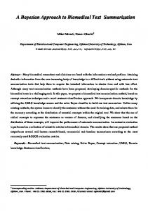
1 Introduction Consider figure 1. What is shown there is the proportion of the times that sentences at particular locations are judged as relevant to summarization, or worthy of inclusion in a summary. Each panel shows judgment results on 25 Japanese texts of a particular genre; columns (G1K3), editorials (G2K3) and news stories (G3K3). All the documents are from a single Japanese news paper, and judgments are elicited from some 100 undergraduate students. While more will be given on the details of the data later (Section 3.2), we can safely ignore them here. Each panel has the horizontal axis representing location or order of sentence in a document, and the vertical axis the proportion of the times sentences at particular locations are picked as relevant to summarization. Thus in G1K3, we see that the first sentence (to appear in a document) gets voted for about 12% of the time, while the 26th sentence is voted for less than 2% of the time. Curiously enough, each of the panels exhibits a distinct pattern in the way votes are spread across
a document: G1K3 has the distribution of votes (DOV) with sharp peaks around 1 and 14; in G2K3, the distribution is peaked around 1, with a small bump around 19; in G3K3, the distribution is sharply skewed to the left, indicating that the majority of votes went to the initial section of a document. What is interesting about the DOV is that we could take it as indicating a collective preference for what to extract for a summary. A question is then, can we somehow exploit the DOV in summarization? To our knowledge, no prior work seems to exist that addresses the question. The paper discusses how we could do this under a Bayesian modeling framework, where we explicitly represent and make use of the DOV by way of Dirichlet posterior (Congdon, 2003).1
2 Bayesian Model of Summaries Since the business of extractive summarization, such as one we are concerned with here, is about ranking sentences according to how useful/important they are as part of summary, we will consider here a particular ranking scheme based on the probability of a sentence being part of summary under a given DOV, i.e., P (y|vv ), (1) where y denotes a given sentence, and v = (v1 , . . . , vn ) stands for a DOV, an array of observed vote counts for sentences in the text; v1 refers to the count of votes for a sentence at the text initial position, v2 to that for a sentence occurring at the second place, etc. Thus given a four sentence long text, if we have three people in favor of a lead sentence, two in favor 1
See Yu et al. (2004) and Cowans (2004) for its use in IR.
249 Proceedings of Human Language Technology Conference and Conference on Empirical Methods in Natural Language c Processing (HLT/EMNLP), pages 249–256, Vancouver, October 2005. 2005 Association for Computational Linguistics
1
4
7 10
14
18
22
26
0.30 0.25 0.20 0.00
0.05
0.10
0.15
votes won (%)
0.25 0.20 0.00
0.05
0.10
0.15
votes won (%)
0.25 0.20 0.15 0.00
0.05
0.10
votes won (%)
g3k3
0.30
g2k3
0.30
g1k3
1
4
7 10
sentences
14
18
22
26
1
4
7 10
sentences
14
18
22
sentences
Figure 1: Genre-by-genre vote distribution of the second, one for the third, and none for the fourth, then we would have v = (3, 2, 1, 0). Now suppose that each sentence yi (i.e., a sentence at the i-th place in the order of appearance) is associated with what we might call a prior preference factor θi , representing how much a sentence at a particular position is favored as part of a summary in general. Then the probability that yi finds itself in a summary is given as: φ(yi |θi )P (θi ),
(2)
where φ denotes some likelihood function, and P (θi ) a prior probability of θi . Since the DOV is something we could actually observe about θi , we might as well couple θi with v by making a probability of θi conditioned on v . Formally, this would be written as: φ(yi |θi )P (θi |vv ).
(3)
The problem, however, is that we know nothing about what each θi looks like, except that it should somehow be informed by v . A typical Bayesian solution to this is to ‘erase’ θi by marginalizing (summing) over it, which brings us to this: Z P (yi |vv ) = φ(yi |θi )P (θi |vv ) dθi . (4) Note that equation 4 no longer talks about the probability of yi under a particular θi ; rather it talks about the expected probability for yi with respect to a preference factor dictated by v . All we need to know
250
v
/ θ
 / yi
Figure 2: A graphical view about P (θi |vv ) to compute the expectation is v and a probability distribution P , and not θi ’s, anymore. We know something about v , and this would leave us P . So what is it? In principle it could be any probability distribution. However largely for the sake of technical convenience, we assume it is one component of a multinomial distribution known as the Dirichlet distribution. In particular, we talk about Dirichlet(θθ |vv ), namely a Dirichlet posterior of θ, given observations v , where θ = P (θ1 , . . . , θi , . . . , θn ), and ni θi = 1 (θi > 0). (Remarkably, if P (θ) is a Dirichlet, so is P (θ|vv ).) θ here represents a vector of preference factors for n sentences — which constitute the text.2 Accordingly, equation 4 could be rewritten as: Z P (yi |vv ) = φ(yi |θθ )P (θθ |vv ) dθθ . (5) An interesting way to look at the model is by way of a graphical model (GM), which gives some intuitive idea of what the model looks like. In a GM perspective, our model is represented as a simple tripartite structure (figure 2), in which each node corresponds to a variable (parameter), and arcs represent 2 Since texts generally vary in length, we may set n to a sufficiently large number so that none of texts of interest may exceed it in length. For texts shorter than n, we simply add empty sentences to make them as long as n.
dependencies among them. x → y reads ‘y depends on x.’ An arc linkage between v and yi is meant to represent marginalization over θ . Moreover, we will make use of a scale parameter λ ≥ 1 to have some control over the shape of the distribution, so we will be working with Dirichlet(θ|λ v ) rather than Dirichlet(θ|vv ). Intuitively, we might take λ as representing a degree of confidence we have in a set of empirical observations we call v , as increasing the value of λ has the effect of reducing variance over each θi in θ. The expectation and variance of Dirichlet(θθ |vv ) are given as follows.3 vi (6) E[θi ] = v0 V ar[θi ] =
vi (v0 − vi ) , v02 (v0 + 1)
(7)
Pn where v0 = i vi . Therefore the variance of a scaled Dirichlet is: V ar[θi |λvv ] =
vi (v0 − vi ) . v02 (λv0 + 1)
(8)
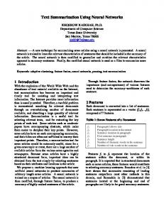
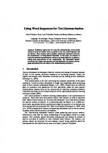
See how λ is stuck in the denominator. Another obvious fact about the scaling is that it does not affect the expectation, which remains the same. To get a feel for the significance of λ, consider figure 3; the left panel shows a histogram of 50,000 variates of p1 randomly drawn from Dirichlet(p1 , p2 |λc1 , λc2 ), with λ = 1, and both c1 and c2 set to 1. The graph shows only the p1 part but things are no different for p2 . (The x-dimension represents a particular value p1 takes (which ranges between 0 and 1) and the y-dimension records the number of the times p1 takes that value.) We see that points are spread rather evenly over the probability space. Now the right panel shows what happens if you increase λ by a factor of 1,000 (which will give you P (p1 , p2 |1000, 1000)); points take a bell shaped form, concentrating in a small region around the expectation of p1 . In the experiments section, we will return to the issue of λ and discuss how it affects performance of summarization. Let us turn to the question of how to find a solution to the integral in equation 5. We will be concerned here with two standard approaches to the issue: one is based on MAP (maximum a posteriori) 3
http://www.cis.hut.fi/ahonkela/dippa/dippa.html
251
and another on numerical integration. We start off with a MAP based approach known as Bayesian Information Criterion or BIC. For a given model m, BIC seeks an analytical approximation for equation 4, which looks like the following: ln P (yi |m) = ln φ(yi |θˆ, m) −
k ln N, 2
(9)
where k denotes the number of free parameters in m, and N that of observations. θˆ is a MAP estimate of θ under m, which is E[θθ ]. It is interesting to note that BIC makes no reference to prior. Also worthy of note is that a minus of BIC equals MDL (Minimum Description Length). Alternatively, one might take a more straightforward (and fully Bayesian) approach known as the Monte Carlo integration method (MacKay, 1998) (MC, hereafter) where the integral is approximated by: n 1X P (yi |vv ) ≈ φ(yi |x(j) ), (10) n j=1
where we draw each sample x(j) randomly from the distribution P (θθ |vv ), and n is the number of x(i) ’s so collected. Note that MC gives an expectation of P (yi |vv ) with respect to P (θθ |vv ). Furthermore, φ could be any probabilistic function. Indeed any discriminative classifier (such as C4.5) will do as long as it generates some kind of probability. Given φ, what remains to do is essentially training it on samples bootstrapped (i.e., resampled) from the training data based on θ — which we draw from Dirichlet(θθ |vv ).4 To be more specific, suppose that we have a four sentence long text and an array of probabilities θ = (0.4, 0.3, 0.2, 0.1) drawn from a Dirichlet distribution: which is to say, we have a preference factor of 0.4 for the lead sentence, 0.3 for the second sentence, etc. Then we resample with replacement lead sentences from training data with the probability of 0.4, the second with the probability of 0.3, and so forth. Obviously, a 4
It is fairly straightforward to sample from a Dirichlet posterior by resorting to a gamma distribution, which is what is happening here. In case one is working with a distribution it is hard to sample from, one would usually rely on Markov chain Monte Carlo (MCMC) or variational methods to do the job.
L=1000
1500 1000 0
500
Frequency
300 0
100
Frequency
500
L=1
0.0
0.2
0.4
0.6
0.8
1.0
0.46
p1
0.48
0.50
0.52
0.54
p1
Figure 3: Histograms of random draws from Dirichlet(p1 , p2 |λc1 , λc2 ) with λ = 1 (left panel), and λ = 1000 (right panel). high preference factor causes the associated sentence to be chosen more often than those with a low preference. Thus given a text T = (a, b, c, d) with θ = (0.4, 0.3, 0.2, 0.1), we could end up with a data set dominated by a few sentence types, such as T 0 = (a, a, a, b), which we proceed to train a classifier on in place of T . Intuitively, this amounts to inducing the classifier to attend to or focus on a particular region or area of a text, and dismiss the rest. Note an interesting parallel to boosting (Freund and Schapire, 1996) and the alternating decision tree (Freund and Mason, 1999). In MC, for each θ (k) drawn from Dirichlet(θθ |vv ), we resample sentences from the training data using probabilities specified by θ (k) , use them for training a classifier, and run it on a test document d to find, for each sentence in d, its probability of being a ‘pick’ (summary-worthy) sentence,i.e., P (yi |θθ (k) ), which we average across θ ’s. In experiments later described, we apply the procedure for 20,000 runs (meaning we run a classifier on each of 20,000 θ ’s we draw), and average over them to find an estimate for P (yi |vv ). As for BIC, we generally operate along the lines of MC, except that we bootstrap sentences using only E[θθ ], and the model complexity term, namely, − k2 ln N is dropped as it has no effect on ranking sentences. As with MC, we train a classifier on the bootstrapped samples and run it on a test document. Though we work with a set of fixed parameters, a bootstrapping based on them still fluctuates, produc-
252
ing a slightly different set of samples each time we run the operation. To get a reasonable convergence in experiments, we took the procedure to 5,000 iterations and averaged over the results. Either with BIC or with MC, building a summarizer on it is a fairly straightforward matter. Given a document d and a compression rate r, what a summarizer would do is simply rank sentences in d based on P (yi |vv ) and pick an r portion of highest ranking sentences.
3 Working with Bayesian Summarist 3.1 C4.5 In what follows, we will look at whether and how the Bayesian approach, when applied for the C4.5 decision tree learner (Quinlan, 1993), leverages its performance on real world data. This means our model now operates either by n
1X P (yi |vv ) ≈ φc4.5 (yi |x(j) ), n
(11)
j=1
or by k ln P (yi |m) = ln φc4.5 (yi |θˆ, m) − ln N, 2
(12)
with the likelihood function φ filled out by C4.5. Moreover, we compare two versions of the classifier; one with BIC/MC and one without. We used Weka implementations of the algorithm (with default settings) in experiments described below (Witten and Frank, 2000).
While C4.5 here is configured to work in a binary (positive/negative) classification scheme, we run it in a ‘distributional’ mode, and use a particular class membership probability it produces, namely, the probability of a sentence being positive, i.e., a pick (summary-worthy) sentence, instead of a category label. Attributes for C4.5 are broadly intended to represent some aspects of a sentence in a document, an object of interest here. Thus for each sentence ψ, its encoding involves reference to the following set of attributes or features. ‘LocSen’ gives a normalized location of ψ in the text, i.e., a normalized distance from the top of the text; likewise, ‘LocPar’ gives a normalized location of the paragraph in which ψ occurs, and ‘LocWithinPar’ records its normalized location within a paragraph. Also included are a few length-related features such as the length of text and sentence. Furthermore we brought in some language specific feature which we call ’EndCue.’ It records the morphology of a linguistic element that ends ψ, such as inflection, part of speech, etc. In addition, we make use of the weight feature (‘Weight’) for a record on the importance of ψ based on tf.idf. Let ψ = w1 , . . . , wn , for some word wi . Then the weight W (ψ) is given as: W (ψ) =
X
(1 + log(tf(w))) · log(N/df(w)).
w
Here ‘tf(w)’ denotes the frequency of word w in a given document, ‘df(w)’ denotes the ’document frequency’ of w, or the number of documents which contain an occurrence of w. N represents the total number of documents.5 Also among the features used here is ‘Pos,’ a feature intended to record the position or textual order of ψ, given by how many sentences away it occurs from the top of text, starting with 0. While we do believe that the attributes discussed above have a lot to do with the likelihood that a given sentence becomes part of summary, we choose not to consider them parameters of the Bayesian model, just to keep it from getting unduly complex. Recall the graphical model in figure 2. 5
Although one could reasonably argue for normalizing W (ψ) by sentence length, it is not entirely clear at the moment whether it helps in the way of improving performance.
253
3.2 Test Data Here is how we created test data. We collected three pools of texts from different genres, columns, editorials and news stories, from a Japanese financial paper (Nihon Keizai Shinbun) published in 1995, each with 25 articles. Then we asked 112 Japanese students to go over each article and identify 10% worth of sentences they find most important in creating a summary for that article. For each sentence, we recorded how many of the subjects are in favor of its inclusion in summary. On average, we had about seven people working on each text. In the following, we say sentences are ‘positive’ if there are three or more people who like to see them in a summary, and ‘negative’ otherwise. For convenience, let us call the corpus of columns G1K3, that of editorials G2K3 and that of news stories G3K3. Additional details are found in table 1.
4 Results and Discussion Tables 2 through 4 show how the Bayesian summarist performs on G1K3, G2K3, and G3K3. The tables list results in precision at compression rates (r) of interest (0 < r < 1). The figures thereof indicate performance averaged over leave-one-out cross validation folds. What this means is that you leave out one text for testing and use the rest for training, which you repeat for each one of the texts in the data. Since we have 25 texts for each data set, this leads to a 25-fold cross validation. Precision is defined by the ratio of hits (positive sentences) to the number of sentences retrieved, i.e., r-percent of sentences in the text.6 In each table, figures to the left of the vertical line indicate performance of summarizers with BIC/MC and those to the right that of summarizers without them. Parenthetical figures like ‘(5K)’ and ‘(20K)’ indicate the number of iterations we took them to: thus BIC(5K) refers to a summarizer based on C4.5/BIC with scores averaged over 5,000 runs. BSE denotes a reference summarizer based on a regular C4.5, which it involves no resampling of training data. LEAD refers to a summarizer which works 6 We do not use recall for a evaluation measure, as the number of positive instances varies from text to text, and may indeed exceed the length of a summary under a particular compression rate.
Table 1: N represents the number of sentences in G1K3 to G3K3. Sentences with three or more votes in their favor are marked positive, that is, for each sentence marked positive, at least three people are in favor of including it in a summary. Genre G1K3 G2K3 G3K3
N 426 558 440
Positive (≥ 3) 67 93 76
Negative 359 465 364
P/N Ratio 0.187 0.200 0.210
Table 2: G1K3. λ = 5. Dashes indicate no meaningful results. r 0.05 0.10 0.15 0.20 0.25 0.30
BIC (5K) 0.4583 0.4167 0.3333 0.2757 0.2525 0.2368
MC (20K) 0.4583 0.4167 0.3472 0.2861 0.2772 0.2535
BSE − − − − − −
LEAD 0.3333 0.3472 0.2604 0.2306 0.2233 0.2066
r 0.05 0.10 0.15 0.20 0.25 0.30
Table 3: G2K3. λ = 5. BIC (5K) MC (20K) BSE 0.6000 0.5800 0.4200 0.4200 0.4200 0.3533 0.3427 0.3560 0.2980 0.3033 0.3213 0.2780 0.2993 0.2776 0.2421 0.2743 0.2750 0.2170
LEAD 0.5400 0.3933 0.3147 0.2767 0.2397 0.2054
r 0.05 0.10 0.15 0.20 0.25 0.30
Table 4: G3K3. λ = 5. BIC (5K) MC (20K) BSE 0.9600 0.9600 0.8400 0.7600 0.7600 0.6800 0.6133 0.6000 0.5867 0.5233 0.5233 0.4967 0.4367 0.4367 0.3960 0.4033 0.4033 0.3640
LEAD 0.9600 0.7000 0.5133 0.4533 0.3840 0.3673
0 (411.0/65.0)
Figure 4: A non Bayesian C4.5 trained on G1K3.
254
LenSenA 114
72 0 (8.0)
=5
0 (5.0/1.0)
1.707 LocSen
1 (3.0/1.0)
0 LenSenA 110
1 (17.0)
LocSen 0.333
0 (3.0)
1 (2.0)
Figure 5: A Bayesian (MC) C4.5 trained on G1K3. by selecting sentences from the top of the text. It is generally considered a hard-to-beat approach in the summarization literature. Table 4 shows results for G3K3 (a news story domain). There we find a significantly improvement to performance of C4.5, whether it operates with BIC or MC. The effect is clearly visible across a whole range of compression rates, and more so at smaller rates. Table 3 demonstrates that the Bayesian approach is also effective for G2K3 (an editorial domain), outperforming both BSE and LEAD by a large margin. Similarly, we find that our approach comfortably beats LEAD in G1K3 (a column domain). Note the dashes for BSE. What we mean by these, is that we obtained no meaningful results for it, because we were unable to rank sentences based on predictions by BSE. To get an idea of how this happens, let us look at a decision tree BSE builds for G1K3, which is shown in figure 4. What we have there is a decision tree consisting of a single leaf.7 Thus for whatever sentence we feed to the tree, it throws back the same membership probability, which is 65/411. But then this would make a BSE based summarizer utterly useless, as it reduces to generating a summary by picking at random, a particular portion of text.8 7
This is not at all surprising as over 80% of sentences in a non resampled text are negative for the most of the time. 8 Its expected performance (averaged over 106 runs) comes
255
Now Figure 5 shows what happens with the Bayesian model (MC), for the same data. There we see a tree of a considerable complexity, with 24 leaves and 18 split nodes. Let us now turn to the issues with λ. As we might recall, λ influences the shape of a Dirichlet distribution: a large value of λ causes the distribution to have less variance and therefore to have a more acute peak around the expectation. What this means is that increasing the value of λ makes it more likely to have us drawing samples closer to the expectation. As a consequence, we would have the MC model acting more like the BIC model, which is based on MAP estimates. That this is indeed the case is demonstrated by table 5, which gives results for the MC model on G1K3 to G3K3 at λ = 1. We see that the MC behaves less like the BIC at λ = 1 than at λ = 5 (table 2 through 4). Of a particular interest in table 5 is G1K3, where the MC suffers a considerable degradation in performance, compared to when it works with λ = 5. G2K3 and G3K3, again, witness some degradation in performance, though not as extensive as in G1K3. It is interesting that at times the MC even works better with λ = 1 than λ = 5 in G2K3 and G3K3.9 to: 0.1466 (r = 0.05), 0.1453 (r = 0.1), 0.1508 (r = 0.15), 0.1530 (r = 0.2), 0.1534 (r = 0.25), and 0.1544 (r = 0.3). 9 The results suggest that if one like to have some improvement, it is probably a good idea to set λ to a large value. But
Table 5: MC (20K). λ = 1. r 0.05 0.10 0.15 0.20 0.25 0.30
G1K3 0.3333 0.3333 0.2917 0.2549 0.2480 0.2594
G2K3 0.5400 0.3867 0.3960 0.3373 0.2910 0.2652
G3K3 0.9600 0.7800 0.5867 0.5200 0.4347 0.4100
All in all, the Bayesian model proves more effective in leveraging performance of the summarizer on a DOV exhibiting a complex, multiply peaked form as in G1K3 and G2K3, and less on a DOV which has a simple, single-peak structure as in G3K3 (cf. figure 1).10
5
Concluding Remarks
The paper showed how it is possible to incorporate information on human judgments for text summarization in a principled manner through Bayesian modeling, and also demonstrated how the approach leverages performance of a summarizer, using data collected from human subjects. The present study is motivated by the view that that summarization is a particular form of collaborative filtering (CF), wherein we view a summary as a particular set of sentences favored by a particular user or a group of users just like any other things people would normally have preference for, such as CDs, books, paintings, emails, news articles, etc. Importantly, under CF, we would not be asking, what is the ‘correct’ or gold standard summary for document X? – the question that consumed much of the past research on summarization. Rather, what we are asking is, what summary is popularly favored for X? Indeed the fact that there could be as many summaries as angles to look at the text from may favor in general how to best set λ requires some experimenting with data and the optimal value may vary from domain to domain. An interesting approach would be to empirically optimize λ using methods suggested in MacKay and Peto (1994). 10 Incidentally, summarizers, Bayesian or not, perform considerably better on G3K3 than on G1K3 or G2K3. This happens presumably because a large portion of votes concentrate in a rather small region of text there, a property any classifier should pick up easily.
256
the CF view of summary: the idea of what constitutes a good summary may vary from person to person, and may well be influenced by particular interests and concerns of people we elicit data from. Among some recent work with similar concerns, one notable is the Pyramid scheme (Nenkova and Passonneau, 2004) where one does not declare a particular human summary a absolute reference to compare summaries against, but rather makes every one of multiple human summaries at hand bear on evaluation; Rouge (Lin and Hovy, 2003) represents another such effort. The Bayesian summarist represents yet another, whereby one seeks a summary most typical of those created by humans.
References Peter Congdon. 2003. Bayesian Statistical Modelling. John Wiley and Sons. Philip J. Cowans. 2004. Information Retrieval Using Hierarchical Dirichlet Processes. In Proc. 27th ACM SIGIR. Yoav Freund and Llew Mason. 1999. The alternating decision tree learning algorithm,. In Proc. 16th ICML. Yoav Freund and Robert E. Schapire. 1996. Experiments with a new boosting algorithm. In Proc. 13th ICML. Chin-Yew Lin and Eduard Hovy. 2003. Automatic evaluation of summaries using n-gram co-occurance statistics. In Proc. HLT-NAACL 2003. David J. C. MacKay and Linda C. Bauman Peto. 1994. A Hierarchical Dirichlet Language Model. Natural Language Engineering. D. J. C. MacKay. 1998. Introduction to Monte Carlo methods. In M. I. Jordan, editor, Learning in Graphical Models, Kluwer Academic Press. Ani Nenkova and Rebecca Passonneau. 2004. Evaluation Content Selection in Summarization: The Pyramid Method. In Proc. HLT-NAACL 2004. J. Ross Quinlan. 1993. C4.5: Programs for Machine Learning. Morgan Kaufmann. Ian H. Witten and Eibe Frank. 2000. Data Mining: Practical Machine Learning Tools and Techniques with Java Implementations. Morgan Kaufmann. Kai Yu, Volker Tresp, and Shipeng Yu. 2004. A Nonparametric Hierarchical Bayesian Framework for Information Filtering. In Proc. 27th ACM SIGIR.