BAYESIAN LEARNING WITH WASSERSTEIN

BAYESIAN LEARNING WITH WASSERSTEIN BARYCENTERS JULIO BACKHOFF-VERAGUAS, JOAQUIN FONTBONA, GONZALO RIOS, FELIPE TOBAR

Abstract. We introduce a novel paradigm for Bayesian learning based on optimal transport theory. Namely, we propose to use the Wasserstein barycenter of the posterior law on models as a predictive posterior, thus introducing an alternative to classical choices like the maximum a posteriori estimator and the Bayesian model average. We exhibit conditions granting the existence and statistical consistency of this estimator, discuss some of its basic and specific properties, and provide insight into its theoretical advantages. Finally, we introduce a novel numerical method which is ideally suited for the computation of our estimator, and we explicitly discuss its implementations for specific families of models. This method can be seen as a stochastic gradient descent algorithm in the Wasserstein space, and is of independent interest and applicability for the computation of Wasserstein barycenters. We also provide an illustrative numerical example for experimental validation of the proposed method. Keywords: Bayesian learning, non-parametric estimation, Wasserstein distance, Wasserstein barycenter, Fréchet means, consistency, gradient descent, stochastic gradient descent.

1. Introduction Consider samples D = {x1 , . . . , xn } in a data space X and a set of feasible models or probability measures M on X. Learning a model m ∈ M from D consists in choosing an element m ∈ M that best explains the data as generated by m, under some given criterion. We adopt the Bayesian viewpoint, which provides a probabilistic framework to deal with model uncertainty, in terms of a prior distribution Π on the space M of models; we refer the reader to [21, 32] and references therein for mathematical background on Bayesian statistics and methods. A critical challenge in the Bayesian perspective, is that of calculating a predictive law on X from the posterior distribution on M, usually referred to as the predictive posterior. This shall be the learning task to which this work is devoted. Our motivation is to find an alternative, non-parametric learning strategy which can cope with some of the drawbacks of standard approaches such as maximum a posteriori (MAP) or Bayesian model average (BMA). The first and main conceptual contribution of our work is the introduction of the Bayesian Wasserstein barycenter estimator (BWB) as a novel model-selection criterion based on optimal transport theory. This is our non-parametric model-selection alternative to MAP and BMA. In a nutshell, given a prior on models Π and observations D = {x1 , . . . , xn } ⊆ X, a BWB estimator is any minimizer m ˆ np ∈ M of the loss function R M 3 m 7→ P(X) W p (m, m) ¯ p Πn (dm), (1.1) where P(X) denotes the set of probability measures on X, Πn is the posterior distribution on models given the data D, and W p is the celebrated p-Wasserstein distance ([38, 39]). In fact we shall consider in Section 2 a general framework for Bayesian estimation based on loss functions over probability measures. This allows us to cover both finitely-parametrized and parameter-free model spaces, and also to retrieve classical selection criteria including MAP, Bayesian model average estimators and generalizations thereof, as particular instances of Fréchet means ([41]) with respect to suitable metrics/divergences on the space of probability measures. Then, in Sections 3.1 and 3.2, we recall the notions of Wasserstein distances and, relying on the previously developed framework, we rigorously introduce the Bayesian Wasserstein barycenter estimator. We explore its existence, uniqueness, absolute continuity, and prove that our estimator has less variance than the Bayesian model average. 1

2

JULIO BACKHOFF-VERAGUAS, JOAQUIN FONTBONA, GONZALO RIOS, FELIPE TOBAR

The second main contribution of our work, carried out in Section 3.3 and culminating in Theorem 3.11, refers to the statistical consistency for the BWB estimator m ˆ np . See [16, 21], and references therein, for a detailed treatment on posterior consistency. Assuming the observations are independent and identically distributed like m0 , we will provide sufficient conditions guaranteeing that lim W p (m ˆ np , m0 ) = 0 (a.s.)

n→∞

This is a highly desirable feature of our estimator, both from a semi-frequentist perspective as well as from the “merging of opinions” point of view in the Bayesian framework (cf. [21, Chapter 6]). The main mathematical difficulty in our analysis comes from the fact that the data space X is, in general, an unbounded metric space. The underlying tools that we employ are the celebrated Schwartz theorem ([37], [21, Proposition 6.16]) on one hand, and the concentration of measure phenomenon for averages of unbounded random variables (e.g., [31, Corollary 2.10]) on the other hand. The minimization of functionals akin to (1.1) is an active field of current research. For instance, if the model space M equals the set of all probability measures on X, then our estimator m ˆ np coincides with the (population) Wasserstein barycenter of Πn . The study of Wasserstein barycenters was introduced by [1], but see also [29, 9] for more recent developments and references to the literature, or our own Appendix B. The third and final main contribution of our work pertains a new algorithm which is ideally suited for the computation of the BWB estimator, and more generally for Wasserstein barycenters. Current numerical methods allowing to compute minimizers of the functional (1.1), and therefore to compute the BWB estimator in particular, are mostly conceived for the case when the prior Π (and hence the posteriors Πn ) has a finite support. Among these methods we stress the contributions [3, 41]. For obvious reasons this leads us to find a method which can directly deal with the general case when the support of Π or Πn is infinite. Our contribution in this regard is the development of an algorithm which can be seen as a stochastic gradient descent method on Wasserstein space; see Sections 4.3 and 4.4. Crucially, we will establish the almost sure convergence of our stochastic algorithm under given conditions in Theorem 4.7 and Proposition 4.11. Our stochastic gradient descent method, just like all other algorithms for the computation of Wasserstein barycenters, takes for granted the availability of optimal transport maps between any two regular probability measures. For this reason we shall present in Section 5 examples of model-families for which these optimal maps are explicitly given. These families also serve to illustrate how the iterations of our stochastic descent algorithm simplify. We close the article with a comprehensive numerical experiment. On the one hand, this serves to illustrate the advantages of the Bayesian Wasserstein barycenter estimator over the Bayesian model average. On the other hand, this experiment suggests as well that the stochastic gradient descent method is a superior alternative for the computation of the Bayesian Wasserstein barycenter estimator, when compared to the more conventional empirical barycenter estimator (cf. Section 4.1). Let us establish the required notation and conventions. We assume throughout the whole article that M ⊆ Pac (X) ⊆ P(X), where P(X) denotes the set of probability measures on X, and Pac (X) is the subset of absolutely continuous measures with respect to a common reference σ-finite measure λ on X. As a convention, we shall use the same notation for an element m(dx) ∈ M and its density m(x) with respect to λ. Finally, given a measurable map T : Y → Z and a measure ν on Y we denote by T (ν) the image measure (or push-forward), which is the measure on Z given by T (ν)(·) = ν(T −1 (·)). We denote by supp(ν) the support of a measure ν and by |supp(ν)| its cardinality.

BAYESIAN LEARNING WITH WASSERSTEIN BARYCENTERS

3

2. Bayesian learning in the model space Consider a fixed prior probability measure Π on the model space M, namely Π ∈ P(M). Assuming as customary that, conditionally on the choice of model m, the data x1 , . . . , xn ∈ X are distributed as i.i.d. observations from the common law m, we can write Π(dx1 , . . . , dxn |m) = m (x1 ) · · · m (xn ) λ(dx1 ) · · · λ(dxn ).

(2.1)

By virtue of the Bayes rule, the posterior distribution Π(dm|x1 , . . . , xn ) on models given the data, which is denoted for simplicity Πn (dm), is given by Πn (dm) :=

m (x1 ) · · · m (xn ) Π (dm) Π (x1 , . . . , xn |m) Π (dm) =R . Π (x1 , . . . , xn ) (x ) (x ) (d m ¯ · · · m ¯ Π m) ¯ 1 n M

(2.2)

The density Λn (m) of Πn (dm) with respect the prior Π(dm) is called the likelihood function. Given the model space M, a loss function L : M × M → R is a non-negative functional. We interpret L(m0 , m) ¯ as the cost of selecting model m ¯ ∈ M when the true model is m0 ∈ M. With a loss function and the posterior distribution over models, we define the Bayes risk (or expected loss) R(m|D) ¯ and a Bayes estimator m ˆ L as follows: R RL (m|D) ¯ := M L(m, m)Π ¯ n (dm) , (2.3) m ˆL

∈

argminm∈M RL (m|D). ¯ ¯

(2.4)

Since both L and Πn operate directly on the model space, model learning according to the above equations does not depend on geometric aspects of parameter spaces. Moreover, the above point of view allows us to define loss functions in terms of various metrics/divergences directly on the space P(X), and therefore to enhance the classical Bayesian estimation framework, by using in particular optimal transportation distances. Before further developing these ideas, we briefly describe how this general framework includes model spaces which are finitely parametrized, and discuss standard choices in that setting, together with their appealing features and drawbacks. This could be helpful for readers who are used to parametrically-defined models. The parametric setting is useful as well, since it helps to illustrate the drawbacks of maximum likelihood estimation (MLE). If the reader is already comfortable with the present non-parametric setup, and is aware of the drawbacks of MLE, he or she may skip Section 2.1 altogether. 2.1. Parametric setting. We say that M is finitely parametrized if there is integer k, a set Θ ⊆ Rk termed parameter space, and a (measurable) function T : Θ 7→ Pac (X), called parametrization mapping, such that M = T (Θ); in such case we denote the model as mθ := T (θ). If the model space M is finitely parametrized, learning a model boils down to finding the best model parameters θ ∈ Θ. This is usually done in a frequentist fashion through the maximum likelihood estimator. We next illustrate the role of the aboveintroduced objects in a standard learning application. Example 2.1. In linear regression, data consist of input (zi ) and output (yi ) pairs, that is, xi = (zi , yi ) ∈ Rq × R for i = 1, . . . , n, and the model space is given by the set of joint distributions p(z, y) = p(y|z)p(z) with linear relationship between y and z. If we moreover assume that y|z is normally distributed, then p(y|z) = N(y; z> β, σ2 ) for some fixed β ∈ Rq and σ2 > 0. In this setting we need to choose the parameters β, σ2 and p(z) to obtain the joint distribution p(z, y), ie. the generative model, though one often needs to deal with the conditional distribution p(y|z), ie. the discriminative model. Hence, for each fixed p0 ∈ Pac (Rq ), the parameter space Θ = Rq × R+ induces a model space M through the mapping (β, σ) 7→ T (β, σ), where T (β, σ) has the density N(y; z> β, σ2 )p0 (z), (z, y) ∈ Rq × R. Conditioning this joint density p(y, z) with respect to a new input z? , we obtain the predictive distribution addressing the regression problem p(y|z? ). In particular, denoting y = (y1 , . . . , yn )> ∈ Rn and Z = (z1 , . . . , zn )> ∈ Rn×q , the MLE parameters are ˆ > (y − Z β). ˆ then given by βˆ = (Z > Z)−1 Z > y and σ ˆ 2 = 1 (y − Z β) n

4


Given p ∈ P(Θ) a prior distribution over a parameter space Θ, its push-forward through the map T is the probability measure Π = T (p) given by Π(A) = p(T −1 (A)). Expressing the likelihood function Λn (m) in terms of the parameter θ such that T (θ) = m, we then easily recover from (2.2) the standard posterior distribution over the parameter space, p(dθ|x1 , . . . , xn ). Moreover, any loss function L induces a functional ` defined on Θ × Θ ˆ = L(mθ0 , mθˆ ), interpreted as the cost of choosing parameter θˆ (and vice versa) by `(θ0 , θ) when the actual true parameter is θ0 . The Bayes risk [7] of θ¯ ∈ Θ is then defined by R R ¯ ¯ R` (θ|D) = Θ `(θ, θ)p(dθ|x ¯ n (dm), (2.5) 1 , . . . , xn ) = M L(m, m)Π where Πn (dm) = Λn (m)Π(dm), with the prior distribution Π = T (p). The associated Bayes ¯ estimator is of course given by θˆ` ∈ argminθ∈Θ R` (θ|D). ¯ ¯ = 1 − δθ¯ (θ) yields R`0−1 (θ|D) ¯ For illustration, consider the 0-1 loss defined as `0−1 (θ, θ) = ¯ 1− p(θ|D), that is, the corresponding Bayes estimator is the posterior mode, also referred to as Maximum a Posteriori Estimator (MAP), θˆ`0−1 = θˆ MAP . For continuous-valued quantities ¯ = kθ − θk ¯ 2 is often preferred. The corresponding Bayes the use of a quadratic loss `2 (θ, θ) R estimator is the posterior mean θˆ`2 = Θ θp(dθ|D). In one dimensional parameter space, the ¯ = |θ − θ| ¯ yields the posterior median estimator. absolute loss `1 (θ, θ) The MAP approach is computationally appealing as it reduces to an optimization problem in a finite dimensional space. The performance of this method might however be highly sensitive to the choice of the initial condition used in the optimization algorithm [40]. This is a critical drawback, since likelihood functions over parameters may be populated with numerous local optima. A second drawback of this method is that it fails to capture global information of the model space, which might result in an overfit of the predictive distribution. Indeed, the mode can often be a very poor summary or atypical choice of the posterior distribution (e.g. the mode of an exponential density is 0, irrespective of its parameter). Yet another serious failure of MAP estimation is its dependence on the parameterization. Indeed, for instance, in the case of a Bernoulli distribution on {0, 1} with p(y = 1) = µ and an uniform prior on [0, 1] for µ, the mode can be anything in [0, 1]. On the other hand, parameterizing the model by θ = µ1/2 yields the mode 1, while parametrizing it by θ = 1 − (1 − µ)1/2 yields 0 as mode. Using general Bayes estimators on parametrized models enables for a richer choice of criteria for model selection (by integrating global information of the parameter space) while providing a measure of uncertainty (through the Bayes risk value). However, this approach might also neglect parametrization related issues, such as overparametrization of the model space (we say that T overparametrizes M if it is not one-to-one). The latter might result in a multi-modal posterior distribution over parameters. For example, take X = Θ = R, m0 = N(x; µ, 1) and T (θ) = N(x|θ2 , 1). If we choose a symmetric prior p(θ), e.g. p(θ) = N(θ|0, 1), then with enough data, the posterior distribution is symmetric with modes near {µ, −µ}, so both `1 and `2 estimators are close to 0. By the above issues, we propose using free-parameter selection criteria via loss functions that compare directly distributions instead of their parameters. 2.2. Posterior average estimators. The next result, proved in Appendix A, illustrates the fact that many Bayesian estimators, including the classic model average estimator, correspond to finding a so-called Fréchet mean or barycenter [41] under a suitable metric/divergence on probability measures. Proposition 2.2. Let M = Pac (X) and consider the loss functions L(m, m) ¯ given by: R 2 1 ¯ λ(dx), i) The L2 -distance: L2 (m, m) ¯ = 2 X (m(x) − m(x)) R ii) The reverse Kullback-Leibler divergence: DKL (m||m) ¯ = X m(x) ln m(x) λ(dx), m(x) ¯ R m(x) ¯ iii) The forward Kullback-Leibler divergence DKL (m||m) ¯ = X m(x) ¯ ln m(x) λ(dx), 2 R √ √ 1 2 iv) The squared Hellinger distance H (m, m) ¯ = 2 X m(x) − m(x) ¯ λ(dx).


5

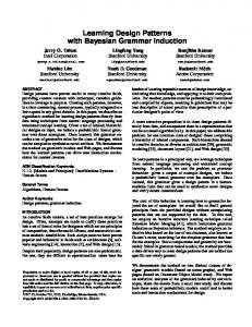
Then, in cases i) and ii) the corresponding Bayes estimators of Equation (2.4) coincide with the Bayesian model average: R m(x) ¯ := EΠn [m] = M m(x)Πn (dm). (2.6) Furthermore, with Ze xp and Z2 denoting normalizing constants, the Bayes estimators corresponding to the cases iii) and iv) are given by the exponential model average and the square model average, respectively: 2 R √ R 1 (2.7) exp M ln m(x)Πn (dm) , m ˆ 2 (x) = Z12 M m(x)Πn (dm) . m ˆ exp (x) = Zexp All the above-described Bayesian estimators (Eqs. (2.6) and (2.7)) share a common feature: their values at each point x ∈ X are computed in terms of some posterior average of the values of certain functions evaluated at x. This is due to the fact that all the above distances are vertical [36], in the sense that computing the distance between m and m ¯ involves the integral of vertical displacements between the graphs of these two densities. An undesirable fact about vertical averages is that they do not preserve properties of the original model space. For example, if the posterior distribution is equally concentrated on two different models m0 = N(µ0 , 1) and m1 = N(µ1 , 1) with µ0 , µ1 , that is, both models are unimodal (Gaussian) with unit variance, the model average is in turn a bimodal (non-Gaussian) distribution with variance strictly greater than 1. More generally, model averages might yield intractable representations or be hardly interpretable in terms of the prior and parameters. We shall next introduce the analogous objects in the case of Wasserstein distances, which are horizontal distances [36], in the sense that they involve integrating horizontal displacements between the graphs of the densities. We will further develop the theory of the corresponding Bayes estimators, which will correspond to Wasserstein barycenters arising in optimal transport theory (see [1, 35, 25, 29]). Going back to the Gaussian example, say for two models given by the univariate Gaussian distributions m0 = N(µ0 , σ20 ) and m1 = N(µ1 , σ21 ), it turns out that the so-called 2-Wasserstein barycenter distribution is σ0 +σ1 2 1 given by m ˆ = m 12 = N( µ0 +µ 2 , ( 2 ) ). In Fig. 1 we illustrate for the reader’s convenience a vertical and a horizontal interpolation between two Gaussian densities. 0.8 0.7 0.6 0.5 0.4 0.3 0.2 0.1 0.00

N(2, 0.5 2 ) N(4, 0.5 2 )

Bayesian Model Average

1

2

3

4

5

0.8 0.7 0.6 0.5 0.4 0.3 0.2 0.1 6 0.00

N(2, 0.5 2 ) N(4, 0.5 2 )

Wassestein Barycenter

1

2

3

4

5

6

Figure 1. Vertical interpolation (left) and horizontal interpolation (right) of two Gaussian densities.

3. The Bayesian Wasserstein barycenter estimator We propose a novel Bayesian estimator obtained by using the Wasserstein distance as loss function. This estimator is therefore given by a Fréchet mean in the Wasserstein metric and, therefore, it is usually referred to as Wasserstein barycenter [1]. For a summary of the notion of Wasserstein barycenters we refer to Appendix B. We state conditions for the statistical consistency of our estimator, which is a basic desirable property: briefly put, this means that as more data becomes available, the estimator converges to the true model. The main result in this regard is Theorem 3.11. We then illustrate the advantage of this estimator by comparing it to the Bayesian model average: it turns out that our estimator is less dispersed, and in particular, it has less variance than the model average. From now until the end of the article, unless otherwise stated, we assume: Assumption 3.1. (X, d) is a separable locally-compact geodesic space and p ≥ 1.

6


Geodesic means that is complete and any pair of points admit a mid-point with respect to d. The reader can think of X as a Euclidean space with d the Euclidean distance. On the other hand d p will control the tail of the models to be considered. We now recall some elements of optimal transport theory. 3.1. Optimal transport and Wasserstein distances in a nutshell. A thorough introduction of optimal transport and some of its applications can be found in the books by Villani [38, 39]. It is difficult to overstate the impact that the field has had in mathematics as a whole. In particular, regarding statistical applications, we refer to the recent survey [33] and the many references therein. In parallel, optimal transport has become increasingly popular within the machine learning community [28], though most of the published works have focused on the discrete setting (e.g., comparing histograms in [15], classification in [20] and images in [13, 6], among others). Let us briefly review definitions and results needed to present our approach. Given two measures µ, υ over X we denote by Γ(µ, υ) the set of couplings with marginals µ and υ, i.e. γ ∈ Γ(µ, υ) if γ ∈ P(X × X) and we have that γ(dx, X) = µ(dx) and γ(X, dy) = υ(dy). Given a real number p ≥ 1 we define the p-Wasserstein space W p (X) by n o R W p (X) := η ∈ P(X) : X d(x0 , x) p η(dx) < ∞, some x0 . The p-Wasserstein between measures µ and υ is given by   1p R   p W p (µ, υ) = inf γ∈Γ(µ,υ) d(x, y) γ(dx, dy) .

(3.1)

X×X

An optimizer of the right-hand side of (3.1) is called an optimal transport. The quantity W p defines a distance turning W p (X) into a complete metric space. In the Euclidean case, there often exist explicit formulae for the optimal transport and the Wasserstein distance, e.g., for the generic one-dimensional case, and for the multivariate Gaussian case with p = 2 (see [14]). If in (3.1) we assume that p = 2, X is Euclidean space, and µ is absolutely continuous, then Brenier’s theorem [38, Theorem 2.12(ii)] establishes the uniqueness of a minimizer. Furthermore, this optimizer is supported on the graph of the gradient of a convex function. 3.2. Wasserstein population barycenter. We start with the definition of Wasserstein population barycenter: Definition 3.2. Given Γ ∈ P(P(X)), the p-Wasserstein risk of m ¯ ∈ P(X) is Z V p (m) ¯ := W p (m, m) ¯ p Γ(dm). P(X)

Any measure m ˆ p ∈ M which is a minimizer of the problem inf V p (m), ¯

m∈M ¯

is called a p-Wasserstein population barycenter of Γ over M. In the case M = W p (X), the above is nothing but the p-Wasserstein population barycenter of Γ introduced in [9]. The term population is used to emphasize that the support of Γ might be infinite. Let us introduce some required notation. For Γ ∈ P(P(X)) we write Γ ∈ P(W p (X)) if Γ is concentrated on a set of measures with finite moments of order p, and Γ ∈ W p (W p (X)) if furthermore for some (and then all) m ˜ ∈ W p (X) it satisfies R W p (m, m) ˜ p Γ(dm) < ∞. P(X) If Γ is concentrated on measures with finite moments of order p and with density with respect to λ,R then we rather write Γ ∈ P(W p,ac (X)), with the notation Γ ∈ W p (W p,ac (X)) if as before P(X) W p (m, m) ˜ p Γ(dm) < ∞ for some m. ˜ We come to the most important definition (and conceptual contribution) of the article. A Bayesian Wasserstein barycenter estimator is nothing but a p-Wasserstein population barycenter of the posteriors Πn over the model space M:


7

Definition 3.3. Given a prior Π ∈ P(M) ⊆ P(P(X)) and data D = {x1 , . . . , xn } which determines Πn as in (2.2), the p-Wasserstein Bayes risk of m ¯ ∈ W p,ac (X), and a Bayes Wasserstein barycenter estimator m ˆ np over the model space M, are defined respectively by: Z V pn (m|D) ¯ := W p (m, m) ¯ p Πn (dm), (3.2) P(X)

m ˆ np

∈

argmin V pn (m|D). ¯

(3.3)

m∈M ¯

Remark 3.4. Under the standing assumption that X is a locally compact separable geodesic space, the existence of a population barycenter is granted if Γ ∈ W p (W p (X)), see [29, Theorem 2] and Appendix B for our own argument. The latter condition is equivalent to the model average m(dx) ¯ := EP [m] (dx) having a finite p-moment, since R R R W p (δy , m) p Γ(dm) = W (X) X d(y, x) p m(dx)Γ(dm) (3.4) W p (X) p R R = X d(y, x) p W (X) m(dx)Γ(dm), (3.5) p

for any y ∈ X. If M is weakly closed then the same reasoning gives the existence of a p-Wasserstein population barycenter of Γ over M; see Appendix B. We summarize this discussion, for the case Γ = Πn , in a simple statement: Lemma 3.5. If X is a locally compact separable geodesic space, M is weakly closed, and the model average m ¯ n (dx) = EΠn [m] (dx) has a.s. finite p-moment, then a.s. a pWasserstein barycenter estimator m ˆ np over M exists. We remark that even if Π ∈ W p (W p (X)), it may still happen that Πn < W p (W p (X)). In Appendix C we provide a sufficient condition on the prior Π ensuring that a.s. : Πn ∈ W p (W p (X)) for all n, and therefore the existence of a barycenter estimator. With this at hand, we make a set of simplifying assumptions which are supposed to hold from now until the end of the article: Assumption 3.6. M = W p,ac (X), Π ∈ W p (W p,ac (X)), and Πn ∈ W p (W p (X)) a.s. all n. We make an important observation regarding the absolute continuity of the barycenter, which is relevant since the model space M = W p,ac (X) is not weakly closed: The next remark states that in spite of Lemma 3.5 not being applicable, the existence of a barycenter belonging to the model space can still be guaranteed. Remark 3.7. If p = 2, X = Rq , d = Euclidean distance, λ =Lebesgue measure, and o n

Π m :

dm dλ ∞ < ∞ > 0,

(3.6)

then the population barycenter of Πn exists, is unique, and is absolutely continuous. The only delicate point is the absolute continuity. This was proven in [25, Theorem 6.2] for compact finite-dimensional manifolds with lower-bounded Ricci curvature (equipped with the volume measure), but one can read-off the (non-compact but flat) Euclidean case X = Rq from the proof therein. If |supp(Π)| < ∞ then (3.6) can be dropped, as shown in [1] or [25, Theorem 5.1]. We last provide a useful characterization of barycenters, which is a generalization of the corresponding result in [3] where only the case |supp(Π)| < ∞ is covered: Lemma 3.8. Assume p = 2, X = Rq , d = Euclidean distance, λ =Lebesgue measure. Let m ˆ be the unique barycenter of Π. Then there exists a jointly measurable function (m, x) 7→ T m (x) which is λ(dx)Π(dm)-a.s. equal R to the unique optimal transport map from m ˆ to m ∈ W2 (X). Furthermore we have x = T m (x)Π(dm), m(dx)-a.s. ˆ

8


Proof. The existence of a jointly measurable version of the unique optimal maps is proved in [19]. Now assume that the last assertion is not true, so in particular 2 R R 0< x − T m (x)Π(dm) m(dx) ˆ 2 R R R R R = |x|2 m(dx) ˆ −2 xT m (x)Π(dm)m(dx) ˆ + T m (x)Π(dm) m(dx). ˆ On the other hand, we have R 2 i2 R R R h R W2 T m Π(dm) (m) ˆ ,m ¯ Π(dm) ¯ ≤ T m¯ (x) − T m (x)Π(dm) m(dx)Π(d ˆ m) ¯ R R 2 m [T (x)] m(dx)Π(dm) = ˆ 2 R R − T m (x)Π(dm) m(dx), ˆ after a few computations. But, by Brenier’s theorem [38, Theorem 2.12(ii)] we know that R R R (x − T m (x))2 m(dx)Π(dm) ˆ = W2 (m, ˆ m)2 Π(dm). Bringing together these three observations, we deduce R 2 R R W2 T m Π(dm) (m) ˆ ,m ¯ Π(dm) ¯ < W2 (m, ˆ m)2 Π(dm),

and in particular m ˆ cannot be the barycenter.

3.3. Statistical consistency. A natural question is whether our estimator is consistent in the statistical sense (see [37, 16, 21]). In short, consistency corresponds to the convergence of our estimator towards the true model m0 , as we observe more i.i.d. data distributed like m0 . In Bayesian language this is a desirable convergence of opinions phenomenon [21]. Here and in the sequel m(∞) denotes the product probability measure corresponding 0 to the infinite sample {xn }n of i.i.d. data distributed according to m0 . In the setting that concerns us, the correct notion of consistency at the level of the prior is given by: Definition 3.9. The prior Π is said to be p-Wasserstein strongly consistent at m0 if for each open neighbourhood U of m0 in the p-Wasserstein topology of W p (X), we have Πn (U c ) → 0 , m(∞) 0 − a.s. The celebrated Schwartz theorem provides sufficient conditions for strong consistency. See the original [37] or [21, Proposition 6.16] for a more modern treatment. A key ingredient in Schwartz’ approach is the notion of Kullback-Leibler support: Definition 3.10. A measure m0 belongs to the Kullback-Leibler support of Π, denoted m0 ∈ KL (Π) , if Π (m : DKL (m0 ||m) < ε) > 0 for every ε > 0, where DKL (m0 ||m) =

R

log mm0 dm0 .

We are mostly interested in the important question, of whether our Wasserstein barycenter estimator converges to the model m0 , i.e. we are after conditions which guarantee that W p (m ˆ np , m0 ) → 0, m0(∞) a.s. This is evidently linked to the question of strong consistency of the prior. We assume throughout Section 3.3 that m0 ∈ KL(Π) and m0 ∈ M. This implies that the model is correct or well specified as discussed in [8, 23, 26, 27]. This setting could be slightly relaxed in the misspecified framework dealt with in those works by considering the reverse Kullback–Leibler projection on M instead of the true model m0 , i.e. the unique model m ˆ 0 ∈ M that minimizes DKL (m0 ||m ˆ 0 ) over M. We can now state our main result concerning consistency of the barycenter estimator: Theorem 3.11. Suppose that Π fulfils the following conditions: (a) supp(Π) is bounded, namely diam(Π) := sup W p (m, m) ¯ < ∞, m,m∈supp(Π) ¯


9

(b) there is λ0 > 0 and x0 ∈ X such that R p sup X eλ0 d (x,x0 ) dm(x) < +∞. m∈supp(Π)

Then under our standing assumptions (in particular, m0 ∈ KL(Π)) we have that Π is pWasserstein strongly consistent at m0 , W p (Πn , δm0 ) → 0 (m(∞) 0 -a.s.), and the barycenter estimator is consistent in the sense that W p (m ˆ np , m0 ) → 0, m(∞) 0 − a.s. A typical example where the boundedness of the support of Π holds is in the finitely parametrized case, when the parameter space is compact and the parametrization function continuous. We stress that X may be unbounded and still diam(Π) may be finite. The proof of Theorem 3.11 is given at the end of this part. Towards this goal, we start with a rather direct sufficient condition for the convergence of m ˆ np to m0 . We use W p to denote throughout the Wasserstein distance both on W p (W p (X)) and on W p (X), not to make the notation heavier. Proposition 3.12. If W p (Πn , δm0 ) → 0 (m0(∞) -a.s.) then W p (m ˆ np , m0 ) → 0 (m(∞) 0 -a.s.). Proof. We have, by minimality of the barycenter R R W p (Πn , δm0 ) p = M W p (m, m0 ) p Πn (dm) ≥ M W p (m, m ˆ np ) p Πn (dm). On the other hand, W p (m0 , m ˆ np ) p ≤ c W p (m, m ˆ np ) p + c W p (m, m0 ) p , ∀m, where the constant c only depends on p. We conclude by R R W p (m0 , m ˆ np ) p ≤ c M W p (m, m ˆ np ) p Πn (dm) + c M W p (m, m0 ) p Πn (dm) R = c M W p (m, m ˆ np ) p Πn (dm) + c W p (Πn , δm0 ) p ≤ 2c W p (Πn , δm0 ) p . Proposition 3.13. If Π is p-Wasserstein strongly consistent at m0 and supp(Π) is bounded, then W p (Πn , δm0 ) → 0 and in particular W p (m ˆ np , m0 ) → 0 (m(∞) 0 − a.s.). Proof. Let B = {m : W p (m, m0 ) < ε} and ε arbitrary, then R W p (Πn , δm0 ) p = M W p (m, m0 ) p Πn (dm) R R ≤ B W p (m, m0 ) p Πn (dm) + Bc W p (m, m0 ) p Πn (dm) R ≤ ε p + Bc W p (m, m0 ) p Πn (dm). Since ε is arbitrary, we only need to check that the second term goes to zero. Strong consistency implies Πn (Bc ) → 0 (m0(∞) − a.s.), and since supp(Πn ) ⊆ supp(Π), we have R W p (m, m0 ) p Πn (dm) ≤ diam(Π) p Πn (Bc ) → 0 (m(∞) 0 − a.s.). Bc We now provide the proof of Theorem 3.11. If the Wasserstein metric was bounded, the argument would be as in [21, Example 6.20], where the main tool is Hoeffding’s inequality. In general Wasserstein metrics are unbounded if X is itself unbounded, and this forces us to assume Conditions (a) and (b) in Theorem 3.11. The argument still rests on the concentration of measure phenomenon: Proof of Theorem 3.11. We aim to apply Proposition 3.13. First we show that if U is any W p (X)-neighbourhood of m0 then m0(∞) -a.s. we have lim inf n Πn (U) ≥ 1. According to Schwartz Theorem (in the form of [21, Theorem 6.17]), under the assumption that m0 ∈ KL(Π), it is enough to find for each such U a sequence of measurable functions ϕn : Xn → [0, 1] such that

10


(1) ϕn (x1 , . . . , xn ) → 0, m(∞) 0 − a.s, and R 1 n (2) lim supn n log U c m (1 − ϕn )Π(dm) < 0. For this purpose, first we will construct tests {ϕn }n that satisfy the above conditions (Point 1 and Point 2) over an appropriate subbase of neighbourhood, to finally extend it to general neighborhoods. It is known that µk → µ onR W p iff for all continuous functions ψ with |ψ(x)| ≤ K(1 + R d p (x, x0 )), K ∈ R it holds that X ψ(x)dµn (x) → X ψ(x)dµ(x); see [39]. Given such ψ and ε > 0 we define the open set n o R R Uψ,ε := m : X ψ(x)dm(x) < X ψ(x)dm0 (x) + ε . These sets form a subbase for the p-Wasserstein neighborhood system at the distribution m0 , and w.l.o.g. we can assume that K = 1 by otherwise considering Uψ/K,ε/K instead. Given a neighborhood U := Uψ,ε as above, we define the test functions R ( P 1 1n ni=1 ψ(xi ) > X ψ(x)dm0 (x) + 2ε , ϕn (x1 , . . . , xn ) = 0 otherwise. By law of large numbers, m(∞) 0 − a.s : ϕn (x1 , . . . , xn ) → 0, so Point 1 is verified. Point 2 is trivial if r := Π(U c ) = 0, so we assume from now on that r > 0. By the hypothesis of finite p-exponential moment of m ∈ supp(Π), the random variable Z = 1 + d p (X, x0 ) with X ∼ m has a moment-generating function Lm (t) which is finite for all λ0 ≥ t ≥ 0, namely h i R p Lm (t) := Em etZ = et X etd (x,x0 ) dm(x) < +∞. Since all the moments of Z are non-negative, we can bound all the k-moments by h i Em Z k ≤ k!Lm (t)t−k , ∀λ0 ≥ t > 0. Thanks to the above bound, we have R R k |ψ(x)| dm(x) ≤ (1 + d p (x, x0 ))k dm(x) ≤ k!Lm (t)t−k . X X We may apply Bernstein’s inequality in the form of [31, Corollary 2.10] to the random variables {−ψ(xi )}i under the measure m(∞) on XN , obtaining for any α < 0 that i P h R α2 m(∞) ni=1 ψ(xi ) − X ψ(x)dm(x) ≤ α ≤ e− 2(v−cα) , where v := 2nLm (t)t−2 , c := t−1 , and 0 < t ≤ λ0 . Going back to the tests ϕn and using the definition of U c we deduce R R R ε n n 1 Pn m (1 − ϕ )Π(dm) = m ψ(x ) ≤ ψ(x)dm (x) + n i 0 c c i=1 n 2 Π(dm) U U X R R ε n 1 Pn ≤ U c m n i=1 ψ(xi ) ≤ X ψ(x)dm(x) − 2 Π(dm) P h i R R = U c mn ni=1 ψ(xi ) − X ψ(x)dm(x) ≤ − nε 2 Π(dm) n 2 o R 2 ≤ U c exp − nε2 8Lmt(t)+tε Π(dm) 2 2 ≤ r exp − nε2 8 sup c t Lm (t)+tε . m∈U ∩supp(Π)

Under our assumption (b) we conclude as desired that R lim supn 1n log U c mn (1 − ϕn )Π(dm) ≤ − 16 sup

t2 ε2

m∈U c ∩supp(Π)

Lm (t)+2tε

< 0.

Now, a general neighborhood U contains a finite intersection of N ∈ N neighborhoods TN from the subbase, i.e. i=1 Uψi ,εi ⊆ U, so R PN R mn (1 − ϕn )Π(dm) ≤ i=1 mn (1 − ϕn )Π(dm), Uc Uc ψi ,εi

and therefore we may conclude as in the subbase case that Point 2 is verified. All in all we have established that Π is p-Wasserstein strongly consistent at m0 , so we conclude by Proposition 3.13 thanks to our Assumption (a).


11

3.4. Bayesian Wasserstein barycenter versus Bayesian model average. It is illustrative to compare the Bayesian model average with our barycenter estimators. First we show that if the Bayesian model converges, then our estimator converges too. We even have the stronger condition that the posterior distribution converges in W p . Recall that the model average is given by m ¯ n (dx) = EΠn [m] (dx). Lemma 3.14. If m(∞) 0 -a.s. the p-moments of the model average converge to those of m0 ∈ KL (Π), then W p (Πn , δm0 ) → 0 (m(∞) ˆ np , m0 ) → 0 (m(∞) 0 -a.s.). In particular, also W p (m 0 -a.s.). Proof. By [21, Example 6.20] we already know that the prior is strongly consistent at m0 with respect to the weak topology (rather than the p-Wasserstein topology). Notice that R R R R W p (m, δ x ) p Πn (dm) = d(x, z) p m(dz)Πn (dm) = d(x, z) p m ¯ n (dz), so a.s. Πn → δm0 not only weakly but in W p . Conclude by Proposition 3.12.

We now briefly consider the case of Π ∈ W2 (W2,ac (Rq )), M = W2,ac (Rq ), λ = Lebesgue, and d = Euclidean distance. Let m ˆ be its unique population barycenter, and denote by (m, x) 7→ T m (x) a measurable function equal λ(dx)Π(dm) a.e. to the unique optimal Rtransport map from m ˆ to m ∈ W2 (X). As a consequence of Lemma 3.8 we have m ˆ = ( T m Π(dm))(m). ˆ Thanks to this fixed-point property, for all convex functions ϕ with at most quadratic growth, we have R R R Emˆ [ϕ(x)] = X ϕ(x)m(dx) ˆ = X ϕ M T m (x)Π(dm) m(dx) ˆ (3.7) R R R R ≤ X M ϕ(T m (x))Π(dm)m(dx) ˆ = M X ϕ(T m (x))m(dx)Π(dm) ˆ R R R R = M X ϕ(x)m(dx)Π(dm) = X ϕ(x) M m(dx)Π(dm) = Em¯ [ϕ(x)], where m ¯ = EΠ [m] is the Bayesian model average. We have used here Jensen’s inequality and Fubini. Since we can replace Π by Πn in this discussion, we have established that the 2-Wasserstein barycenter estimator is less dispersed than the Bayesian model average: namely, in the convex-order sense. In particular we have established: Lemma 3.15. Let m ¯ n be the Bayesian model average and m ˆ n the 2-Wasserstein barycenter of the posterior Πn . Then we have Em¯ n [x] = Emˆ n [x] and Em¯ n [kxk2 ] ≥ Emˆ n [kxk2 ], so the 2-Wasserstein barycenter estimator has less variance than the model average estimator. 4. On the computation of the population Wasserstein barycenter In this part we discuss possible ways to compute/approximate the population Wasserstein barycenter. This is a crucial step in constructing our Bayesian Wasserstein estimator (see (3.3)). To this effect, we introduce a novel algorithm for computation of barycenters in Section 4.3, which can be seen as a stochastic gradient descent method on Wasserstein space. This is the main contribution of this part of the article, followed by Section 4.4 where we present a generalization of this method (batch stochastic gradient descent). We begin this development in Section 4.1 with a straightforward Monte-Carlo method, which has an illustrative purpose and therefore is not studied in depth. This method motivates us to summarize in Section 4.2 the essentials of the gradient descent method in Wasserstein space, developed in [41, 3], where we can fix important notation and ideas for our main contribution in Sections 4.3 and 4.4. For our results, we assume we are capable of generating independent models mi from the posteriors Πn and the prior Π. In the parametric setting, we can use efficient Markov Chain Monte Carlo (MCMC) techniques [22] or transport sampling procedures [17, 34, 24, 30] to generate models mi sampled from Πn or Π. 4.1. Empirical Wasserstein barycenter. In practice, except in special cases, we cannot calculate integrals over the entire model space M. Thus we must approximate such integrals by e.g., Monte Carlo methods. For this reason, we now discuss the empirical Wasserstein barycenter and its usefulness as an estimator. For a related statement when |supp(Π)| < ∞ see [10, Theorem 3.1].

12

JULIO BACKHOFF-VERAGUAS, JOAQUIN FONTBONA, GONZALO RIOS, FELIPE TOBAR iid

Definition 4.1. Given mi ∼ Πn for i = 1, . . . , k, the empirical measure Π(k) n over models is (k) 1 Pk Πn := k i=1 δmi ∈ P(M) . Note that if a.s. Πn ∈ W p (W p,ac (X)) then a.s. Π(k) n ∈ W p (W p,ac (X)), so all hypothesis (k) (k) about Πn stand on Πn . Using Πn instead of Πn , we define the p-Wasserstein empirical Bayes risk V p(n,k) (m|D), ¯ as well as a corresponding empirical Bayes estimator m ˆ (n,k) p , which in the case M = W p is referred to as a p-Wasserstein empirical barycenter of Πn (see [9]). Remark 4.2. It is known that a.s. Π(k) n converges weakly to Πn as k → ∞. If Πn has finite p-th moments, by the strong law of large numbers we have convergence of p-th moments: R R 1 Pk p W p (m, m0 ) p Π(k) W p (m, m0 ) p Πn (dm) a.s. n (dm) = k i=1 W p (mi , m0 ) → Thus we have that a.s. Π(k) n → Πn in W p as k → ∞. Thanks to [29, Theorem 3], any sequence of empirical barycenters (m ˆ kn )k≥1 of (Πkn )k≥1 converges (up to selection of a subsequence) in p-Wasserstein distance to a (population) barycenter m ˆ n of Πn . Combining these facts, the following result is immediate: Lemma 4.3. If W p (Πn , δm0 ) → 0, m(∞) 0 -a.s., there exists a data-dependent sequence kn := ˆ knn , m0 ) → 0, m(∞) kn (x1 , . . . , xn ) such that (m ˆ knn )n≥1 satisfy W p (m 0 -a.s. Proof. Since W p is a metric we have that W p (m ˆ kn , m0 ) ≤ W p (m ˆ kn , m ˆ n ) + W p (m ˆ n , m0 ) for all (∞) k, n ≥ 0, and thanks to Proposition 3.12 the last term tends to zero m0 -a.s. as n → ∞. Using a diagonal argument, for each m ˆ n exists kn (determined by the data-dependent Πn ) s.t. ˆ knn , m ˆ n ) ≤ 1n , thus obtaining the convergence. the empirical barycenter m ˆ kn satisfies W p (m 4.2. Gradient descent on Wasserstein space. We first survey the gradient descent method for the computation of 2-Wasserstein empirical barycenters. This will serve as a motivation for the subsequent development of the stochastic gradient descent in Sections 4.3 and 4.4. From now until the end of the article we strengthen Assumption 3.6 by further assuming (cf. Remark 3.7) that Assumption 4.4. X = Rq , d = Euclidean metric, λ = Lebesgue measure, p = 2. P Let us consider m1 , . . . , mk ∈ W2,ac (Rq ), weights λ1 , . . . , λk ∈ R+ , ki=1 λi = 1 and the P respective discrete measure1 Π(k) = ki=1 λi δmi . Given some measure m ∈ W2,ac (Rq ), we denote the optimal transport map from m to mi as T mmi for i = 1, . . . , k. The uniqueness and existence of this map is guaranteed by Brenier’s Theorem. With this notation one can define the operator Gk : W2,ac (Rq ) → W2,ac (Rq ) as P Gk (m) := ki=1 λi T mmi (m). (4.1) Owing to [3] the operator Gk is continuous for the W2 distance. Also, if at least one of the mi has a bounded density, then the unique Wasserstein barycenter m ˆ of Π(k) has a bounded density and satisfies Gk (m) ˆ = m. ˆ Thanks to this, starting from µ0 ∈ W2,ac (Rq ) one can define the sequence µn+1 := Gk (µn ), for n ≥ 0.

(4.2)

´ The following result was established by Alvarez-Esteban, del Barrio, Cuesta-Albertos and Matrán in [3, Theorem 3.6], as well as independently by Zemel and Panaretos in [41, Theorem 3,Corollary 2]: The sequence {µn }n≥0 defined in (4.2) is tight and every weakly convergent subsequence of {µn }n≥0 must converge in W2 distance to a measure in W2,ac (Rq ) which is a fixed point of Gk . If some mi has a bounded density, and if Gk has a unique fixed point m, ˆ then m ˆ is the 1One can think of Π(k) as an empirical approximation of the posterior Π or the prior Π. n


13

Wasserstein barycenter of Π(k) and we have that W2 (µn , m) ˆ → 0. The previous result allows one to estimate the barycenter of any discrete measure (i.e. any prior/posterior with a finite support), as long as one is able to construct the optimal transports T mmi . Thanks to the almost Riemannian geometry of the Wasserstein space W2 (Rq ) (see [5, Chapter 8]) one can reinterpret the iterations defined in (4.2) as a gradient descent iteration. This was discovered by Panaretos and Zemel in [41, 33]. In fact, in P [41, Theorem 1] the authors prove the following: Letting Π(k) = ki=1 λi δmi as above, then q the (half) Wasserstein Bayes risk of m ∈ W2,ac (R ) and its Fréchet derivative are given respectively by P (4.3) Fk (m) := 12 ki=1 λi W22 (mi , m), P P Fk0 (m) = − ki=1 λi (T mmi − I) = I − ki=1 λi T mmi , (4.4) where I is the identity map on Rq . It follows by Brenier’s theorem [38, Theorem 2.12(ii)] that m ˆ is a fixed point of Gk defined in (4.1) if and only if Fk0 (m) ˆ = 0 (one says that m ˆ is a Karcher mean of Π(k) ). The gradient descent sequence with step γ ∈ [0, 1] starting from µ0 ∈ W2,ac (Rq ) is defined as µn+1 := Gk,γ (µn ), for n ≥ 0,

(4.5)

where h i Gk,γ (m) : = I + γFk0 (m) (m) h i P = (1 − γ)I + γ ki=1 λi T mmi (m). These ideas by Zemel and Panaretos serve us as an inspiration for the stochastic gradient descent iteration in the next part. Let us finally remark that if γ = 1 the aforementioned gradient descent sequence equals the sequence in (4.2), i.e. Gk,1 = Gk . In fact in [41] the authors prove that the choice γ = 1 is optimal. 4.3. Stochastic gradient descent for population barycenters. The method in Section 4.2 works perfectly well for calculating the empirical barycenter. For the estimation of a population barycenter (i.e. when the prior does not have a finite support) we would need to construct a convergent sequence of empirical barycenters, as in Section 4.1, and then apply the method in Section 4.2. Altogether this can be computationally expensive. To remedy this, we follow the ideas in [12] and define a stochastic version of the gradient descent sequence for the barycenter of Π ∈ W2 (W2,ac (Rq )). Needless to say, Π could represent the posterior or prior distribution. iid

Definition 4.5. Let µ0 ∈ W2,ac (Rq ), mk ∼ Π, and γk > 0 for k ≥ 0. Then we define the stochastic gradient descent sequence as h i (4.6) µk+1 := (1 − γk )I + γk T µmkk (µk ) , for k ≥ 0. By Remark 3.7 and an induction argument, we clearly have {µk }k ⊆ W2,ac (Rq ), a.s.

(4.7)

Let us introduce the key ingredients for the convergence analysis of the stochastic gradient iterations: R (4.8) F(µ) := 12 W (X) W22 (µ, m)Π(dm) 2,ac R F 0 (µ) := − W (X) (T µm − I))Π(dm). (4.9) 2,ac

Observe that the population barycenter µˆ is the minimizer of F and that by Lemma 3.8 also kF 0 (µ)k ˆ L2 (µ) ˆ = 0. The next proposition (cf. [41, Lemma 2]) indicates us that, in expectation, the sequence {F(µk )}k is essentially decreasing for a sufficiently small step γk . This is a first indication of the behaviour of the sequence {µk }k . We denote by {Fk }k the filtration of the i.i.d. sample mk ∼ Π, namely F−1 is the trivial sigma-algebra and Fk+1 is the sigma-algebra generated by m0 , . . . , mk . In this way µk is Fk -measurable.

14


Proposition 4.6. For the stochastic gradient descent sequence in (4.6), we have E F(µk+1 ) − F(µk )|Fk ≤ γk2 F(µk ) − γk kF 0 (µk )k2L2 (µk ) .

(4.10)

Proof. Let ν ∈ supp(Π). By (4.7) we know that h i (1 − γk )I + γk T µmkk , T µνk (µk ), is a feasible (not necessarily optimal) coupling with first and second marginals µk+1 and ν respectively. Denoting Om := T µmk − I, we have W22 (µk+1 , ν) ≤ k(1 − γk )I + γk T µmkk − T µνk k2L2 (µk ) = k−Oν + γk Omk k2L2 (µk ) = kOν k2L2 (µk ) − 2γk hOν , Omk iL2 (µk ) + γk2 kOmk k2L2 (µk ) . Evaluating µk+1 on the functional F and thanks to the previous inequality, we have R F(µk+1 ) = 12 W22 (µk+1 , ν)Π(dν) DR E R γ2 ≤ 12 kOν k2L2 (µ ) Π(dν) − γk Oν Π(dν), Omk 2 + 2k kOmk k2L2 (µ ) L (µk )

k

=F(µk ) + γk F (µk ), Omk

0

L2 (µk )

+

k

γk2 2 2 kOmk kL2 (µk ) .

Taking conditional expectation with respect to Fk , and as mk is independently sampled from this sigma-algebra, we conclude D E R γ2 R E F(µk+1 )|Fk ≤F(µk ) + γk F 0 (µk ), Om Π(dm) 2 + 2k kOm k2L2 (µ ) Π(dm) L (µk )

=(1 +

γk2 )F(µk )

− γk kF

0

k

(µk )k2L2 (µ ) . k

Now we will show that under reasonable assumptions the sequence {F(µk )}k converges a.s. to the unique minimizer of F. As mentioned above, this minimizer is the 2-Wasserstein population barycenter of Π, which we denote µ. ˆ We will need the following convergence result recalled in [11]: (Quasi-martingale convergence theorem) Given a random sequence {ht }t≥0 adapted to the filtration {Ft }, define δt := 1 if E [ht+1 − ht |Ft ] > 0 and δt := 0 otherwise. If ht ≥ 0 for all t ≥ P 0, and the infinite sum of the positive expected variations is finite ( ∞ t=1 E [δt (ht+1 − ht )] < ∞) then the sequence {ht } converges almost surely to some h∞ ≥ 0. We will assume the following conditions over the steps γt appearing in (4.6): P∞ 2 t=1 γt < ∞ P∞ t=1 γt = ∞.

(4.11) (4.12)

Additionally the following conditions will be useful to finish the arguments: W2,ac (X) 3 µ 7→ kF 0 (µ)k2L2 (µ) is lower semicontinuous w.r.t. Wq for some q < 2, (4.13) W2,ac (X) 3 µ 7→ kF 0 (µ)k2L2 (µ) has a unique zero.

(4.14)

We shall examine these conditions in Remark 4.8. Now the main result of this part: Theorem 4.7. Under conditions (4.11) and (4.12) the stochastic gradient descent sequence {µt }t is a.s. relatively compact in Wq for all q < 2 (in particular it is tight). If furthermore (4.13) and (4.14) hold, then a.s. {µt }t≥0 converges to the W2 -population barycenter µˆ of Π in the Wq topology (in particular it weakly converges). Proof. Denote Fˆ := F(µ) ˆ and introduce the sequences Q ˆ ht := F(µt ) − F, αt := t−1 i=1

1 . 1+γi2


15

Observe that ht ≥ 0 for all t. Thanks to condition (4.11) the sequence αt converges to some α∞ > 0, as can be checked by taking logarithm. By Proposition 4.6 we have h i ˆ E ht+1 − (1 + γt2 )ht |Ft ≤ γt2 Fˆ − γt kF 0 (µt )k2 2 ≤ γt2 F, (4.15) L (µt )

so after multiplying by αt+1 we derive the bound ˆ E [αt+1 ht+1 − αt ht |Ft ] ≤ αt+1 γt2 Fˆ − αt+1 γt kF 0 (µt )k2L2 (µt ) ≤ αt+1 γt2 F.

(4.16)

We define δt := 1 if E [αt+1 ht+1 − αt ht |Ft ] > 0 and δt := 0 otherwise. Then P∞ P∞ t=1 E [δt (αt+1 ht+1 − αt ht )] = t=1 E [δt E [αt+1 ht+1 − αt ht |Ft ]] P 2 ˆ P∞ 2 ≤ Fˆ ∞ t=1 αt+1 γt ≤ F t=1 γt < ∞. Since αt ht ≥ 0, by the quasi-martingale convergence theorem {αt ht }t converges almost surely, but as αt converges to α∞ > 0, then ht also converges almost surely to some h∞ ≥ 0. Taking expectations is (4.16), summing in t so that a telescopic sum forms, we have P E[αt+1 ht+1 ] ≤ α0 h0 + Fˆ ts=1 α s+1 γ2s ≤ C. Taking limit inferior, applying Fatou’s lemma, and since α∞ > 0, we conclude E[h∞ ] < ∞. In particular h∞ is a.s. finite. This means that F(µt ) has a finite a.s. limit, which we call L. By convexity of transport costs ([39, Theorem 4.8]) we have R 1 2 W µ , mΠ(dm) ≤ F(µt ) ≤ L + 1, t 2 2 R for t eventually large enough. Since Π ∈ W2 (W2 (Rq )) we have mΠ(dm) ∈ W2 (Rq ), so it follows that the second moments of {µt }t are a.s. bounded by some finite (random) constant M. An application of Markov’s inequality proves that the sequence {µt }t is a.s. tight, since closed balls in Rq are compact. Further, for q < 2, by Hölder and Chebyshev inequalities we have that R R 1 M q kxk dµ ≤ kxk2 dµt ≤ R1−q/2 , t 1−q/2 R kxk>R so {µt }t≥0 is a.s. relatively compact in Wq thanks to [38, Theorem 7.12] and R M lim lim supt→∞ kxk>R kxkq dµt ≤ lim lim supt→∞ R1−q/2 = 0. R→∞

R→∞

Back to (4.16), taking expectations, summing in t to obtain a telescopic sum, we get P P E[αt+1 ht+1 ] − h0 α0 ≤ Fˆ ts=1 α s+1 γ2s − ts=1 α s+1 γ s kF 0 (µ s )k2L2 (µ ) . s

Taking limit inferior, by Fatou on the l.h.s. and monotone convergence on the r.h.s. we get i hP 0 2 −∞ < E[α∞ h∞ ] − h0 α0 ≤ C − E ∞ s=1 α s+1 γ s kF (µ s )kL2 (µ ) . s

In particular, we have P∞ t=1

γt kF 0 (µt )k2L2 (µ ) < ∞, a.s. t

(4.17)

Observe that lim infkF 0 (µt )k2L2 (µ ) > 0 would be at odds with (4.17) and (4.12), so further t

lim infkF 0 (µt )k2L2 (µt ) = 0, a.s. We now assume Conditions (4.13) and (4.14). If some subsequence of {µt }t Wq -converges to some µ , µ, ˆ then along this subsequence we must have lim infkF 0 (µt )k2L2 (µ ) > 0: indeed, t otherwise by (4.13) we would have kF 0 (µ)k2L2 (µ) = 0, contradicting (4.14) since already kF 0 (µ)k ˆ 2L2 (µ) = 0. Since we do know that lim infkF 0 (µt )k2L2 (µ ) = 0 a.s., it follows that realˆ t izations where {µt }t accumulates into a limit different than µˆ have zero measure. Thus a.s. the only possible accumulation point of {µt }t is µ. ˆ In particular, by a.s. relative compactness of {µt }t , this sequence must Wq -converge a.s. to the population barycenter µ, ˆ concluding the proof.

16


Remark 4.8. The validity of (4.14) is equivalent to the uniqueness of an (absolutely continuous) fixed point for the functional R m ¯ 7→ T mm¯ Π(dm) (m), ¯ (4.18) which is in general unsettled. In the finite-support case [1, Remark 3.9] and specially [41, Theorem 2] provide reasonable sufficient conditions. For the infinite-support case the uniqueness of fixed-points, as far as we know, has only been explored in [9, Theorem 5.1] under strong assumptions. It is imaginable that the arguments in [41] can be generalized to the infinite-support case, but we do not explore this in the present work. On the other hand it seems plausible that (4.13) holds in full generality. In this direction we refer to [41, Proposition 3] for a continuity statement when, again, Π has finite support. We give next a sufficient/alternative condition for (4.13) of our own, which does work for the infinite-support case. Proposition 4.9. Assumption (4.13) is fulfilled if (i) X = R. Alternatively, assume that (ii) µ0 ∈ supp(Π) ⊆ H ⊆ W2,ac (Rq ), where H is geodesically closed and closed under composition of optimal maps, meaning respectively2 ∀m, m ˜ ∈ H, ∀α ∈ [0, 1] : ([1 − α]I + αT mm˜ )(m) ∈ H, −1 ∀µ, m, m ˜ ∈ H : T mm¯ = T µm¯ ◦ T µm .

(4.19) (4.20)

Then for the stochastic gradient descent sequence we have a.s. {µk }k ⊆ H. Further the functional H 3 µ 7→ kF 0 (µ)k2L2 (µ) is W2 -continuous and weakly lower semicontinuous, and the conclusions of Theorem 4.7 remain valid if Condition (4.13) is dropped. Proof. We first settle the case of Condition (ii). It is immediate from (4.19) that µ1 ∈ H, and by induction it follows similarly that a.s. {µk }k ⊆ H. We now establish the continuity statement, decomposing the functional as follows 2 R R kF 0 (µ)k2 = T m (y)Π(dm) − y µ(dy) L2 (µ)

X

µ

2 R R R R R = X T µm (y)Π(dm) µ(dy) − 2 X y · T µm (y)µ(dy)Π(dm) + X kyk2 µ(dy). R The term µ 7→ X kyk2 µ(dy) is continuous in W2 and weakly lower semicontinuous. As Brenier maps are optimal, we have R y · T µm (y)µ(dy) = sup E y · z := ρ(µ, m). X y∼µ, z∼m

Thus ρ(·, m) is continuous in W2 and weakly R upper semicontinuous, so under the standing assumption that Π ∈ W2 (W2,ac ) the term ρ(µ, m)Π(dm) is continuous in W2 and weakly upper semicontinuous too. Finally we only have to check that the first term is continuous: i hR i 2 R R R hR T µm (y)Π(dm) µ(dy) = X T µm (y)Π(dm) · T µm˜ (y)Π(dm) ˜ µ(dy) X i R R hR m m ˜ = T (y) · T (y)µ(dy) Π(dm)Π(dm) ˜ µ µ R R X = G(µ, m, m)Π(d ˜ m)Π(dm) ˜ R where G(µ, m, m) ˜ = X T µm (y) · T µm˜ (y)µ(dy). For µ, m, m ˜ ∈ H we have that R m m ˜ G(µ, m, m) ˜ = X T µ (y) · T µ (y)µ(dy) −1 R = X T µm (y) · T µm˜ ◦ T µm ◦ T µm (y) µ(dy) −1 R = X z · T µm˜ ◦ T µm (z) m(dz) R = X z · T mm˜ (z)m(dz), 2Since µ, m are absolutely continuous we have by [38, Theorem 2.12(iv)] T m −1 = T µ , (m − a.s.) m µ


17

thanks to the Condition (4.20). Since G(µ, m, m) ˜ is independent of µ, we conclude that the functional µ 7→ kF 0 (µ)k2L2 (µ) is W2 -continuous and weakly lower semicontinuous on H as desired. With this at hand we can go back to the arguments in the proof of Theorem 4.7, checking their validity without Condition (4.13). Finally let us consider Condition (i). In this case (4.20) is true for all µ, m, m ˜ absolutely continuous, since the composition of increasing functions on the line is increasing. The above arguments verbatim prove the validity of (4.13). Examples where Condition (4.20) are fulfilled are explained in [10, Proposition 4.1], and include the case of radial transformations and component-wise transformations of a base measure. In general (4.20) is rather restrictive, since the composition of gradients of convex functions need not be a gradient of some convex function. 4.4. Batch stochastic gradient descent on Wasserstein space. To generate the sequence iid (4.6) in the k-step, we sampled mk ∼ Π, chose a suitable γk > 0 and then updated µk via the transport map T k := I + γk (T µmkk − I). The expected transport map is R E [T k ] = I + γk (T µmkk − I)Π(dmk ) = I − γk F 0 (µk ). Notice that −(T µmk − I) is an unbiased estimator for F 0 (µ), but in many cases it can have a high variance so the learning rates γ must be very small for convergence. This motivates us to propose alternative estimators for F 0 (µ) with less variance: iid

Definition 4.10. Let µ0 ∈ W2,ac (Rq ), mik ∼ Π, and γk > 0 for k ≥ 0 and i = 1, . . . , S k . The batch stochastic gradient descent sequence is given by P k mik (4.21) T µk (µk ). µk+1 := (1 − γk )I + γk S1k Si=1 Denote this time Fk+1 the sigma-algebra generated by {mi` : ` ≤ k, i ≤ S k }. Notice that P k mik W := S1k Si=1 T µk − I is an unbiased estimator of −F 0 (µk ). Then, much as in Proposition 4.6, we have E F(µk+1 )|Fk R γ2 R =F(µk ) + γk hF 0 (µk ), W Π(dm1k · · · dmSk k )iL2 (µk ) + 2k kWk2L2 (µ ) Π(dm1k · · · dmSk k ) k mik γk2 R 1 PS k 2 1 0 2 =F(µk ) − γk kF (µk )kL2 (µ ) + 2 k S k i=1 T µk − IkL2 (µ ) Π(dmk · · · dmSk k ) k k mik γk2 1 PS k R 0 2 2 ≤F(µk ) − γk kF (µk )kL2 (µ ) + 2 S k i=1 kT µk − IkL2 (µ ) Π(dmik ) k

k

=(1 + γk2 )F(µk ) − γk kF 0 (µk )k2L2 (µ ) . k

From here on it is routine to follow the arguments in the proof of Theorem 4.7, obtaining the following result: Proposition 4.11. Under conditions (4.11) and (4.12) the batch stochastic gradient descent sequence {µt }t is a.s. relatively compact in Wq for all q < 2. If furthermore (4.13) and (4.14) hold, then a.s. {µt }t≥0 converges to the W2 -population barycenter µˆ of Π in the Wq -topology. The main idea of using mini-batch is noise reduction for the estimator of F 0 (µ). The variance of the one-sample estimator where m ∼ Π is h i

h i

2 V[−(T µm − I)] = E k−(T µm − I)k2L2 (µ) −

E −(T µm − I)

2 L (µ) h i

2 2 0

= E W2 (µ, m) − F (µ) L2 (µ) = 2F(µ) − kF 0 (µ)k2L2 (µ) .

18


On the other hand, the variance of the mini-batch estimator where mi ∼ Π for i ≤ S is h i i

2

2

h P P P V − S1 Si=1 (T µmi − I) = E

− S1 Si=1 (T µmi − I)

L2 (µ) −

E − S1 Si=1 (T µmi − I)

2 L (µ)

2 P

m 2 S = E − S1 i=1 (T µ i − I) L2 (µ) − kF 0 (µ)kL2 (µ) For the first term we can expand it as

2 P P P

− S1 Si=1 (T µmi − I)

L2 (µ) = S12 h Si=1 (T µmi − I), Sj=1 (T µm j − I)iL2 (µ) P P m = S12 Si=1 Sj=1 hT µmi − I, T µ j − IiL2 (µ) P P m = S12 Si=1 k−(T µmi − I)k2L2 (µ) + S12 Sj,i hT µmi − I, T µ j − IiL2 (µ) , so if we take expectation, as the samples mi ∼ Π are independent, we have h h h i i i h m i P P P E k− S1 Si=1 (T µmi − I)k2L2 (µ) = S12 Si=1 E W22 (µ, mi ) + S12 Sj,i hE T µmi − I , E T µ j − I iL2 (µ) P P = S22 Si=1 F(µ) + S12 Sj,i hF 0 (µ), F 0 (µ)iL2 (µ) =

2 S F(µ)

+

S −1 0 2 S kF (µ)kL2 (µ) .

Finally the variance of the mini-bath estimator is given by i h i h P V − S1 Si=1 (T µmi − I) = S1 2F(µ) − kF 0 (µ)k2L2 (µ) . Thus we have established: P Proposition 4.12. The variance of the mini batch estimator − S1 Si=1 (T µmi − I) for F 0 (µ) P decreases linearly as the sample size S grows, ergo V[− S1 Si=1 (T µmi − I)] = O( S1 ). 5. On families with closed-form gradient descent step and their barycenters In Section 4 we presented some methods to compute the population Wasserstein barycenter, which assume that we are capable of getting samples from the distributions Π and Πn , and that we can calculate the optimal transports between measures. While sampling is solved by techniques like MCMC, computing optimal transports is not achievable in a general way. For this reason we exhibit in this section some families of distributions for which it is possible to calculate these optimal transports. Furthermore we will examine their barycenter, establishing some properties which are conserved under the operation of taking barycenter. 5.1. Univariate distributions. For a continuous distribution m in R we denote its cumulative distribution function by Fm (x) and its right-continuous quantile function by Qm (·) = Fm−1 (·). The p-Wasserstein optimal transport map from some continuous m0 to m is independent of p and given by the monotone rearrangement (see [38, Remark 2.19(iv)]): T 0m (x) = Qm (Fm0 (x)). Note that this class of functions is closed under composition, convex combination, and contains the identity. Given Π the barycenter m ˆ is also independent of p and characterized by the averaged quantile function, i.e. R Qmˆ (·) = Qm (·)Π(dm). A stochastic gradient descent iteration, starting from a distribution function Fµ (x), sampling some m ∼ Π, and with step γ, produces the measure ν = ((1 − γ)I + γT µm )(µ), which is characterized by its quantile function Qν (·) = (1 − γ)Qµ (·) + γQm (·). A general batch stochastic gradient descent iteration is described by Qν (·) = (1 − γ)Qµ (·) + γ PS i=1 Qmi (·). S


19

It is interesting to note that the model average m ¯ is characterized by the averaged cuR mulative distribution function, i.e. Fm¯ (·) = Fm (·)Π(dm). As we mentioned earlier, the model average does not preserve intrinsic shape properties from the distributions such as symmetry or unimodality. For example if Π = 0.3 ∗ δm1 + 0.7 ∗ δm2 with m1 = N(1, 1) and m2 = N(3, 1), the model average is an asymmetric bimodal distribution with modes on 1 and 3. A continuous distribution m on R is called unimodal with a mode on x˜ ∈ R if its cumulative distribution function F(x) is convex for x < x˜ and concave for x > x˜. One says that m is symmetric around xm ∈ R if F(xm + x) = 1 − F(xm − x) for x ∈ R. One can also characterize unimodality and symmetry by quantile function. A continuous distribution m on R is unimodal with a mode on x˜ if its quantile function Q(y) is concave for y < y˜ and convex for y > y˜ , where Q(˜y) = x˜. Likewise, m is symmetric around xm ∈ R if Q( 12 + y) = 2xm − Q( 12 − y) for y ∈ [0, 12 ]. Thanks to this characterization we conclude that the barycenter preserves unimodality/symmetry: Lemma 5.1. If Π ∈ W p (Pac (R)) is concentrated on symmetric (resp. symmetric unimodal) univariate distributions, then the barycenter m ˆ is symmetric (resp. symmetric unimodal). Proof. Using the quantile function characterization, we have that R i R h Qmˆ 21 + y = Qm 12 + y Π(dm) = 2xm − Qm 12 − y Π(dm) = 2xmˆ − Qmˆ 12 − y , R where xmˆ := xm Π(dm) is the symmetric point, that coincides with the median and the mean of the barycenter. If a symmetric distribution is unimodal, then the mode coincides with the median and mean, i.e Qm ( 12 ) = xm . Since the average of convex (concave) functions is convex (concave), it is clear that the barycenter of symmetric unimodal distributions is also symmetric unimodal. Although the unimodality is not preserved in general non-symmetric cases, there are still many families of distributions in which the unimodality is preserved after taking barycenter, as we show in the next result. Lemma 5.2. If Π ∈ W p (Pac (R)) is concentrated on log-concave univariate distributions, then the barycenter m ˆ is unimodal. Proof. Let f (x) be a log-concave density, then − log( f (x)) is convex so exp(− log( f (x)) = 1 ˜ ∈ R, so quantile function Q(y) f (x) is convex. Necessarily f must be unimodal for some x 1 is concave for y < y˜ and convex for y > y˜ where Q(˜y) = x˜. Since f (x) is convex decreasing 1 is convex. Hence for x < x˜ and convex increasing for x > x˜, then f (Q(y)) convex positive with minima on y˜ . Given Π, its barycenter m ˆ satisfies R dQ dQmˆ m dy = dy Π(dm),

dQ dy (y)

=

1 f (Q(y))

is

dQmˆ m so if all dQ ˆ so Qmˆ (y) is dy are convex, then dy is convex positive with minima on some y concave for y < yˆ and convex for y > yˆ and m ˆ is unimodal with a mode on xˆ = Qmˆ (ˆy).

There are many useful common log-concave distribution families like the normal one, the exponential, logistic, Gumbel, chi-squared, chi and Laplace. Other examples include the Weibull, power, gamma and beta families, when the shape parameters are equal or greater than 1. It is interesting to note that some of these families are closed under taking barycenter. For example, the barycenter of normal distributions is normal, and this remains true for the exponential, logistic, Gumbel and Laplace families. 5.2. Distributions sharing a common copula. If two multivariate distributions P and Q over Rq share the same copula, then their W p (Rq ) distance to the p-th power is the sum of the W p (R) distances between their marginals raised to the p-power. Furthermore, if the marginals of P are continuous, then an optimal map is given by the coordinate-wise transformation T (x) = (T 1 (x1 ), . . . , T q (xq )) where T i (xi ) is the monotone rearrangement between the marginals Pi and Qi for i = 1, . . . , q. Note that these kind of transports are

20


closed under composition, convex combination, and contain the identity. This setting allows us to easily extend the results from the univariate case to the multidimensional case. Lemma 5.3. If Π ∈ W p (Pac (Rq )) is concentrated on a set of measures sharing the same copula C, then the p-Wasserstein barycenter m ˆ of Π has copula C as well, and its i-th marginal m ˆ i is the barycenter of the i-th marginal measures of Π. In particular the barycenter does not depend on p. Proof. It is know [14, 2] that for two distributions m and µ with i-th marginals mi and µi for i = 1, ..., q respectively, the p-Wasserstein metric satisfies P W pp (m, µ) ≥ ni=1 W pp (mi , µi ), where equality is reached if m and µ share the same copula C. (We abuse notation denoting W p the p-Wasserstein distance on Rq as well as on R.) Thus R p R Pq Pq R p p i i i i W p (m, µ)Π(dm) ≥ i=1 W p (m , µ )Π(dm) = i=1 W p (ν, µ )Π (dν), R R where Πi is defined via the identity P(R) f (ν)Πi (dν) = P(Rq ) f (mi )Π(dm). The infimum for the lower bound is reached onR the univariate measures m ˆ 1 , ..., m ˆ q where m ˆ i is the pp i i i i barycenter of Π , i.e. m ˆ = argmin W p (ν, µ )Π (dν). It is plain that the infimum is reached on the distribution m ˆ with copula C and i-th marginal m ˆ i for i = 1, ..., q, which then has to be the barycenter of Π and is independent of p. A stochastic gradient descent iteration, starting from a distribution µ, sampling some m ∼ Π, and with step γ, both µ and m having copula C, produces the measure ν = ((1 − γ)I + γT µm )(µ) characterized by having copula C and the i-th marginal quantile functions Qνi (·) = (1 − γ)Qµi (·) + γQmi (·), for i = 1, . . . , q. The batch stochastic gradient descent iteration works analogously. Alternatively, one can perform (batch) stochastic gradient descent componentwise (with respect to the marginals Πi of Π) and then make use of the copula C. 5.3. Spherically equivalent distributions. Following [14], another useful multidimensional case is constructed as follows: Given a fixed measure m ˜ ∈ W2,ac (Rq ), its associated family of spherically equivalent distributions is o n S0 := S(m) ˜ = L α(kk x˜x˜kk22 ) x˜ |α ∈ ND(R), x˜ ∼ m ˜ , where k k2 is the Euclidean norm and ND(R) is the set of non-decreasing non-negative functions of R+ . These type of distributions include the simplicially contoured distributions, and also elliptical distributions with the same correlation structure. Here and in the sequel we denote by L(·) the law of a random vector, so m = L(x) and x ∼ m are synonyms. If y ∼ m ∈ S0 , then we have that α(r) = Qkyk2 (Fk x˜k2 (r)), where Qkyk2 is the quantile function of the norm of y, Fk x˜k2 is the distribution function of the norm of x˜, and y ∼ α(kk x˜x˜kk22 ) x˜. More generally, if m1 = L α1k(kx˜kx˜2k2 ) x˜ and m2 = L α2k(kx˜kx˜2k2 ) x˜ , then the optimal transport

2) from m1 to m2 is given by T mm12 (x) = α(kxk kxk2 x where α(r) = Qkx2 k2 (F kx1 k2 (r)). Since F kx1 k2 (r) = −1 −1 Fk x˜k2 (α1 (r)) and Qkx2 k2 (r) = α2 (Qk x˜k2 (r)), then α(r) = α2 (Qk x˜k2 (Fk x˜k2 (α−1 1 (r)))) = α2 (α1 (r)), so finally

α (α−1 (kxk ))

2 1 T mm12 (x) = 2 kxk x. 2 Note that these kind of transports are closed under composition, convex combination, and contain the identity. A stochastic gradient descent iteration, starting from a distribution µ = L α0k(kx˜kx˜2k2 ) x˜ , α(k x˜k ) sampling some m = L k x˜k22 x˜ ∼ Π, with step γ, produces the distribution m1 = T 0γ,m (µ) := (γα+(1−γ)α0 )(α−1 0 (kxk2 )) ((1 − γ)I + γT µm )(µ). Since T 0γ,m (x) = x, we have that m1 = L α1k(kx˜kx˜2k2 ) x˜ kxk2 with α1 = γα + (1 − γ)α0 . Analogously, the batch stochastic gradient iteration produces P α1 = (1 − γ)α0 + Sγ Si=1 αmi .


21

Note that these iterations live in S0 , thus, ˆ ∈ S0 . so does the Rbarycenter m α(k ˆ x˜k2 ) m For the barycenter m ˆ = L k x˜k2 x˜ , the equation T mˆ (x)Π(dm) = x can be expressed R R ˆ m as α(r) ˆ = αm (r)Π(dm), or equivalently, Qm Qm kˆyk2 (p) = kyk2 (p)Π(dm), where Qkyk2 is the quantile function of the norm of y ∼ m. Note the similarity with the univariate case. 5.4. Scatter-location family. We borrow here the setting of [4], where another useful multidimensional case is defined as follows: Given a fixed distribution m ˜ ∈ W2,ac (Rq ), referred to as generator, the generated scatter-location family is given by q F0 := F (m) ˜ = {L(A x˜ + b)|A ∈ Mq×q ˜ ∼ m}, ˜ + ,b ∈ R ,x

where Mq×q + is the set of symmetric positive definite matrices of size q × q. Without loss of generality we can assume that m ˜ has zero mean and identity covariance. Note that if m ˜ is the standard multivariate normal distribution, then F (m) ˜ is the multivariate normal distribution family. The optimal map between two members of F0 is explicit. If m1 = L(A1 x˜ + b1 ) and m2 = L(A2 x˜ + b2 ) then the optimal map from m1 to m2 is given by T mm12 (x) = A(x − b1 ) + b2 2 1/2 −1 where A = A−1 A1 ∈ Mq×q + . Observe that this family of optimal transports 1 (A1 A2 A1 ) contains the identity map and is closed under convex combination. If Π is supported on F0 , then its 2-Wasserstein barycenter m ˆ belongs to F0 . In fact m ˆ Since the optimal map from m call its mean bˆ and its covariance matrix Σ. R ˆ to m is T mˆ (x) = m ˆ ˆ −1/2 (Σˆ 1/2 Σm Σˆ 1/2 )1/2 Σˆ −1/2 and we know that T m (x)Π(dm) = x, Am ˆ =Σ m ˆ m ˆ (x− b)+bm where Am R R ˆ = bm Π(dm), Π(dm) = I, since clearly b m-almost ˆ surely. Then weRmust have that Am m ˆ and as a consequence Σˆ = (Σˆ 1/2 Σm Σˆ 1/2 )1/2 Π(dm). A stochastic gradient descent iteration, starting from a distribution µ = L(A0 x˜ + b0 ), sampling some m = L(Am x˜ + bm ) ∼ Π, and with step γ, produces the measure ν = ˜ T 0γ,m (µ) := ((1 − γ)I + γT µm )(µ). If x˜ has a multivariate distribution F(x), then µ has −1 2 ˜ distribution F0 (x) = F(A0 (x − b0 )) with mean b0 and covariance Σ0 = A0 . We have that m −1 2 1/2 −1 T 0γ,m (x) = ((1 − γ)I + γAm A0 . Then µ )(x − b0 ) + γbm + (1 − γ)b0 with Aµ := A0 (A0 Am A0 ) ν has distribution −1 ˜ F1 (x) = F0 ([T 0γ.m ]−1 (x)) = F([(1 − γ)A0 + γAm µ A0 ] (x − γbm − (1 − γ)b0 )),

with mean b1 = (1 − γ)b0 + γbm and covariance 2 1/2 Σ1 = A21 = [(1 − γ)A0 + γA−1 ][(1 − γ)A0 + γ(A0 A2m A0 )1/2 A−1 0 (A0 Am A0 ) 0 ] 2 2 1/2 = A−1 ][(1 − γ)A20 + γ(A0 A2m A0 )1/2 ]A−1 0 [(1 − γ)A0 + γ(A0 Am A0 ) 0 2 2 1/2 2 −1 = A−1 ] A0 0 [(1 − γ)A0 + γ(A0 Am A0 )

The batch stochastic gradient descent iteration is characterized by P b1 = (1 − γ)b0 + Sγ Si=1 bmi γ PS 2 2 1/2 2 −1 A21 = A−1 ] A0 . i=1 (A0 Ami A0 ) 0 [(1 − γ)A0 + S 6. Numerical experiments We next present experimental validation for our theoretical contribution. The aim of this simulation experiment is to provide practical evidence for the implementation of the proposed approach to Wasserstein Bayesian learning and its relationship to the true model. Specifically, the following experiment consists in: i) defining a true model, ii) sampling from such model to yield a set of data points, iii) sampling from the posterior measures, iv) computing the proposed Bayesian 2-Wasserstein barycenter via empirical approximation, v) analysing our estimator with respect to both the true model and the standard Bayesian model average, and lastly, vi) comparing the empirical approximation versus the proposed stochastic gradient methods for computing population barycenters.

22


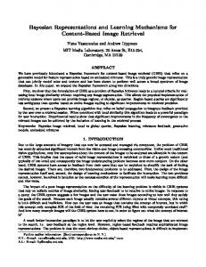
6.1. Choice of the true model, prior and posterior samples. Following the discussion in Sec. 5.4, we considered models within the location-scatter family (LS), since optimal transports between members of the LS can be computed in closed form but are not reduced to the well-known univariate case. We chose the generator of the LS family, denoted m, ˜ as a distribution on R15 with independent coordinates, where: • coordinates 1 to 5 are standard Normal distributions • coordinates 6 to 10 are standard Laplace distributions, and • coordinates 11 to 15 are standard Student’s t-distributions (3 degrees of freedom). Fig. 2 shows uni- and bi-variate marginals for 6 coordinates of m. ˜

normal 2

normal 1

2 0 2 2.5 0.0 2.5

laplace 1

5 0 5

laplace 2

5 0

0 5 10

student-t 2

student-t 1

5

5 0 2.5 0.0 2.5 normal 1

2.50.0 2.5 normal 2

5 0 5 laplace 1

5

0 5 laplace 2

10 0 student-t 1

5

0 5 student-t 2

Figure 2. Univariate (diagonal) and bivariate (off-diagonal) marginals for 6 coordinates from the generator distribution m. ˜ The diagonal and lower triangular plots are smoothed histograms, whereas the upperdiagonal ones are collections of samples. Within the LS family constructed upon m, ˜ we chose the true model m0 to be generated by the location vector b ∈ R15 defined as bi = i − 1 for i = 1, . .. , 15, and the scatter 1.1 j−1 1.1 matrix A = Σ1/2 . The covariance matrix Σ was defined as Σi, j = K i−1 , 14 for 14 i, j = 1, . . . , 15 3, with the kernel function K(i, j) = εδi j + σ cos (ω(i − j)). Given the parameters ε, σ and ω, the so constructed covariance matrix will be denoted Σε,σ,ω . We chose the parameters ε = 0.01, σ = 1 and ω = 5.652 ≈ 1.8π for m0 . Therefore, under the true model m0 the coordinates can be negatively/positively correlated due to the cosine term and there is also a coordinate-independent noise component due to the Kronecker delta δi j . Fig. 3 shows the covariance matrix and three coordinates of the generated true model m0 . The model prior Π is the push-forward induced by the chosen prior over the mean vector b and the parameters of the covariance Σε,σ,ω . We chose all these priors to be independent and given by p(b, Σε,σ,ω ) = N(b|0, I) Exp(ε|20) Exp(σ|1) Exp(ω−1 |15), 3We chose j−1 1.1 for j = 1, . . . , 15 because this defines a non-uniform grid over [0, 1]. 14

(6.1)


1.00 0.75

2

5 dim 1

0

23

0

0.50

4

0.25

10

0.00 8

dim 8

6

5 0

0.25 10

0.75

14 0

2

4

6

8

10

12

14

dim 15

0.50 12

20 10

0 5 dim 1

0

dim 8

10

10

20 dim 15

Figure 3. True model m0 : covariance matrix (left), and univariate and bivariate marginals for dimensions 1, 8 and 15 (right). Notice that some coordinates are positively or negatively correlated, and some are even close to be uncorrelated. where Exp(·|λ) is a exponential distribution with rate λ. Given n samples from the true model m0 (also referred to as observations or data points), we generated k samples from the posterior measure Πn using Markov chain Monte Carlo (MCMC), all to obtain the empirical measure Π(k) n . The remaining part of our numerical analysis focuses on the behavior of the Bayesian Wasserstein barycenter as a function of both the number of samples k and the number of data points n. 6.2. Numerical consistency of the empirical posterior under the Wasserstein distance. We first validated the empirical measure Π(k) n , as a consistent sample version of the true posterior under the W2 distance, that is, we would like to confirm that W2 (Π(k) n , δm0 ) → W2 (Πn , δm0 ) for large k. In this sense, we estimated W2 (Π(k) n , δm0 ) 10 times for each combination of (number of) observations n and samples k in the following sets • k ∈ {1, 5, 10, 20, 50, 100, 200, 500, 1000} • n ∈ {10, 20, 50, 100, 200, 500, 1000, 2000, 5000, 10000} Fig. 4 shows the 10 estimates of W2 (Π(k) n , δm0 ) for different values of k (in the x-axis) and of n (color coded). Notice how the estimates become more concentrated for larger k and that the Wasserstein distance between the empirical measure Πn(k) and the true model m0 decreases for larger n. Additionally, Table 1 shows that the standard deviation of the 10 estimates of W2 (Π(k) n , δm0 ) decreases as either n or k increases. 6.3. Distance between the empirical barycenter and the true model. For each empirˆ (k) ical posterior Π(k) n we intend to compute their Wasserstein barycenter m n as suggested in (k) Section 4.1. We call m ˆ n the empirical barycenter. For this purpose, we use the iterative procedure defined in (4.2), namely the (deterministic) gradient descent method, and repeated this calculation 10 times. As a stopping criterion for the gradient descent method, we considered the relative variation of the W2 cost, terminating the computation if this quantity was less than 10−4 . Fig. 5 shows all the W2 distances between the so computed barycenters and the true model, while Table 2 shows the average across all these distances for each pair (n, k). Notice that, in general, both the average and standard deviation of the barycenters decrease as either n or k increases, yet for large values (e.g., n = 2000, 5000) numerical issues appear.

24


2

0

n 10.0 20.0 50.0 100.0 200.0 500.0 1000.0 2000.0 5000.0 10000.0

log_w2

2

4

6

1.0

5.0

10.0

20.0

50.0 k

100.0

200.0

500.0

1000.0

Figure 4. Wasserstein distance between the empirical measure Π(k) n and δm0 in logarithmic scale for different number of observations n (color coded) and samples k (x-axis). For each pair (n, k), 10 estimates of W2 (Π(k) n , δm0 ) are shown. Table 1. Standard deviation of W22 (Π(k) n , δm0 ), using 10 simulations, for different values of observations n and samples k. n/k 10 20 50 100 200 500 1000 2000 5000 10000

1 1.2506 1.5168 0.3479 0.2003 0.0749 0.0478 0.0299 0.0145 0.0072 0.0038

5 0.8681 0.5691 0.0948 0.1092 0.1249 0.0285 0.0113 0.0071 0.0031 0.0020

10 0.5880 0.3524 0.1275 0.0712 0.0717 0.0093 0.0113 0.0040 0.0015 0.0005

20 0.9690 0.3182 0.0572 0.0469 0.0533 0.0086 0.0064 0.0031 0.0018 0.0005

50 0.2354 0.1850 0.0623 0.0431 0.0393 0.0053 0.0067 0.0027 0.0010 0.0004

100 0.3440 0.1841 0.0229 0.0254 0.0101 0.0056 0.0036 0.0019 0.0007 0.0004

200 0.1253 0.1049 0.0157 0.0087 0.0092 0.0045 0.0016 0.0014 0.0004 0.0002

500 0.1330 0.0811 0.0085 0.0079 0.0109 0.0023 0.0012 0.0011 0.0005 0.0002

1000 0.0972 0.0509 0.0092 0.0084 0.0072 0.0022 0.0007 0.0006 0.0002 0.0001

6.4. Distance between the empirical barycenter and the Bayesian model average. Our aim was then to compare the computed empirical Wasserstein barycenters m ˆ (k) n to the stan(k) dard Bayesian model averages m ¯ n , in terms of their distance to the true model m0 , for n = 1000 observations. In order to do so, we estimated the W2 distances via empirical approximations with 1000 samples for each model based on [18]. We simulated this procedure 10 times for k ∈ {10, 20, 50, 100, 200, 500, 1000}. Fig. 6 shows the sample average and variance of the W2 distances of the Wasserstein barycenters and Bayesian model averages, where it can be seen that the empirical barycenter is closer to the true model than the model average regardless of the number of MCMC samples k. 6.5. Computation of the barycenter using batches. Lastly, we compared the empirical barycenters m ˆ (k) n against the barycenter obtained by our batch stochastic gradient descent method m ˆ n,s . Fig. 7 shows the evolution of the W22 distance between the stochastic gradient descent sequences and the true model m0 for n ∈ {10, 20, 50, 100, 200, 500, 1000} observations and batches of sizes s ∈ {1, 15}, with step-size γt = 1t for t = 1, . . . , 200. This means


25

0

log_baricenter_m0

2

n 10.0 20.0 50.0 100.0 200.0 500.0 1000.0 2000.0 5000.0 10000.0

4

6

10.0

20.0

50.0

100.0

k

200.0

500.0

1000.0

2000.0

Figure 5. W2 distance between the empirical barycenters m ˆ (k) n and the true model m0 in logarithmic scale for different number of observations n (color coded) and samples k (x-axis). For each pair (n, k), 10 estimates of W2 (m ˆ (k) n , m0 ) are shown. Table 2. Sample average of W22 (m ˆ (k) n , m0 ), using 10 simulations, for different values of observations n and samples k. n/k 10 20 50 100 200 500 1000 2000 5000 10000

10 2.1294 1.4382 0.2455 0.1211 0.1116 0.0094 0.0068 0.0072 0.0037 0.0023

20 2.0139 1.4498 0.2759 0.1387 0.0922 0.0077 0.0039 0.0066 0.0037 0.0017

50 2.0384 1.4826 0.2639 0.1509 0.0859 0.0043 0.0031 0.0063 0.0028 0.0017

100 1.9396 1.4973 0.2468 0.1458 0.0817 0.0047 0.0025 0.0062 0.0029 0.0015

200 1.9608 1.4785 0.2499 0.1379 0.0777 0.0041 0.0023 0.0063 0.0031 0.0016

500 1.9411 1.4953 0.2483 0.1328 0.0824 0.0038 0.0022 0.0060 0.0031 0.0017

1000 1.9699 1.4955 0.2443 0.1318 0.0820 0.0037 0.0021 0.0062 0.0028 0.0016

2000 1.9548 1.4914 0.2454 0.1349 0.0819 0.0039 0.0021 0.0062 0.0030 0.0017

that, for batch size s and a number of observations equal to n, we carry out 200 iterations of the batch stochastic gradient method (4.21) with these explicit step-sizes {γt }t : the resulting estimator is m ˆ n,s . Notice from Fig. 7 that the larger the batch, the more concentrated the trajectories of m ˆ n,s become, and that the estimates exhibit random fluctuations when the batch size is small. Additionally, Table 3 summarizes the means of the distance W22 to the true model m0 , using the sequences after t = 100 against the empirical estimator using all the simulations with k ≥ 100. Finally, Table 4 shows the standard deviation of the distance W22 to the true model m0 , where we can notice that the standard deviation decreases as the batch size grows. Critically, observe that for batch sizes s ≥ 5 the stochastic estimation is better than its empirical counterpart, i.e. it has lower variance with similar (or less) bias. This is noteworthy given the fact that computing our Wasserstein barycenter estimator via the batch stochastic gradient descent method is computationally less demanding than computing it via the empirical method. Based on this illustrative numerical example, we can conclude that:


• the empirical posterior constructed using MCMC sampling is consistent under the W2 distance and therefore can be relied upon to compute Wasserstein barycenters, • the empirical Wasserstein barycenter estimator tends to converge faster (and with lower variance) to the true model than the empirical Bayesian model average, • computing the population Wasserstein barycenter estimator via batch stochastic gradient descent seems to be a superior alternative to computing the empirical barycenter (i.e., to applying the deterministic gradient descent method to a finitely sampled posterior).

2.00 1.75 1.50 1.25 w2

26

model ma wb

1.00 0.75 0.50 0.25 0.00

10.0

20.0

50.0

100.0 k

200.0

500.0

1000.0

Figure 6. Averages (bars) and standard deviations (vertical lines) of 2 W22 (m ˆ (k) ¯ (k) n , m0 ) denoted as WB in orange, and W2 (m n , m0 ) denoted as MA in blue, for n = 1000 and different numbers of samples k. We considered 10 simulations for each k.

Table 3. Means of W22 of the stochastic gradient estimations (using the sequences with t ≥ 100) and that of the empirical estimator (using the simulations with k ≥ 100), across different combinations of observations n and batch size s. n/s 10 20 50 100 200 500

1 2.0421 1.4819 0.2406 0.1340 0.0843 0.0044

2 2.0091 1.4868 0.2512 0.1392 0.0811 0.0042

5 1.9549 1.5100 0.2465 0.1340 0.0819 0.0039

10 1.9721 1.4852 0.2427 0.1349 0.0807 0.0039

15 1.9732 1.4840 0.2444 0.1334 0.0820 0.0041

20 1.9712 1.4891 0.2460 0.1338 0.0819 0.0040

empirical 1.9532 1.4916 0.2469 0.1366 0.0811 0.0041

Table 4. Std. deviations of W22 of the stochastic gradient estimations (using the sequences with t ≥ 100) and that of empirical estimator (using the simulations with k ≥ 100), across different combinations of observations n and batch size s. n/s 10 20 50 100 200 500 1000

1 0.1836 0.0751 0.0210 0.0102 0.0074 0.0016 0.0005

2 0.1071 0.0565 0.0174 0.0076 0.0045 0.0007 0.0006

5 0.0526 0.0553 0.0072 0.0049 0.0021 0.0005 0.0004

10 0.0474 0.0189 0.0084 0.0048 0.0035 0.0004 0.0004

15 0.0397 0.0253 0.0050 0.0035 0.0013 0.0004 0.0003

20 0.0232 0.0186 0.0039 0.0023 0.0017 0.0004 0.0003

empirical 0.0916 0.0790 0.0138 0.0112 0.0047 0.0009 0.0005


n = 10 | s = 1

2.5

n = 10 | s = 15

2.5

2.0

2.0 0

25

50

75

100

125

150

175

0

25

50

n = 20 | s = 1 1.75

1.50

1.50 0

25

50

75

100

125

150

175

1.25

0

25

50

n = 50 | s = 1 0.30

0.25

0.25 0

25

50

75

100

125

150

175

n = 100 | s = 1

0.175

100

125

150

175

75

100

125

150

175

150

175

150

175

150

175

150

175

150

175

n = 50 | s = 15

0.30

0.20

75

n = 20 | s = 15

1.75 1.25

27

0.20

0

25

50

0.175

0.150

75

100

125

n = 100 | s = 15

0.150

0.125

0.125 0

25

50

75

100

125

150

175

0

25

50

n = 200 | s = 1 0.10

0.10

0.08

0.08 0

25

50

75

100

125

150

175

0

25

50

n = 500 | s = 1 0.006

0.004

0.004 25

50

75

100

125

150

175

0

25

50

n = 1000 | s = 1 0.004

0.002

0.002 25

50

75

100

125

125

75

100

125

75

100

125

n = 1000 | s = 15

0.004

0

100

n = 500 | s = 15

0.006

0

75

n = 200 | s = 15

150

175

0

25

50

75

100

125

Figure 7. Evolution of the W22 cost for 10 realizations of the stochastic barycenter and their mean (blue) versus an empirical barycenter estimator (red), for n = 10, 20, 50, 100, 200, 500, 1000 and batches sizes s = 1, 15. Acknowledgements We thank financial support from Conicyt #AFB170001 Center for Mathematical Modeling (GR, JF and FT), Fondecyt-Iniciacion #11171165 (FT), Conicyt-Pcha/DocNac/201621161789 (GR), Nucleo Milenio NC 130062 (JF) and Fondecyt Regular #1150570 (JF). Part of this work was carried out during a visit by GR to JB, which was partially funded by the FWF-grant #Y00782. We thank Mathias Beiglböck and the Vienna University of Technology for this support and their hospitality. References [1] Martial Agueh and Guillaume Carlier. Barycenters in the Wasserstein space. SIAM Journal on Mathematical Analysis, 43(2):904–924, 2011. [2] Aurélien Alfonsi and Benjamin Jourdain. A remark on the optimal transport between two probability measures sharing the same copula. Statistics & Probability Letters, 84:131–134, 2014.

28


´ [3] Pedro C Alvarez-Esteban, Eustasio del Barrio, Juan A Cuesta-Albertos, and Carlos Matrán. A fixedpoint approach to barycenters in Wasserstein space. Journal of Mathematical Analysis and Applications, 441(2):744–762, 2016. ´ [4] Pedro C Alvarez-Esteban, Eustasio del Barrio, Juan A Cuesta-Albertos, and Carlos Matrán. Wide consensus aggregation in the Wasserstein space. application to location-scatter families. Bernoulli, 24(4A):3147–3179, 2018. [5] Luigi Ambrosio, Nicola Gigli, and Giuseppe Savaré. Gradient flows: in metric spaces and in the space of probability measures. Springer Science & Business Media, 2008. [6] Martin Arjovsky, Soumith Chintala, and Léon Bottou. Wasserstein generative adversarial networks. In Proceedings of the International Conference on Machine Learning, volume 70, pages 214–223. PMLR, 2017. [7] James O Berger. Statistical decision theory and Bayesian analysis. Springer Science & Business Media, 2013. [8] Robert H Berk et al. Limiting behavior of posterior distributions when the model is incorrect. The Annals of Mathematical Statistics, 37(1):51–58, 1966. [9] Jérémie Bigot and Thierry Klein. Characterization of barycenters in the Wasserstein space by averaging optimal transport maps. arXiv preprint arXiv:1212.2562, 2012. [10] Emmanuel Boissard, Thibaut Le Gouic, and Jean-Michel Loubes. Distribution’s template estimate with Wasserstein metrics. Bernoulli, 21(2):740–759, 2015. [11] Léon Bottou. Online learning and stochastic approximations. On-line learning in neural networks, 17(9):142, 1998. [12] Léon Bottou, Frank E Curtis, and Jorge Nocedal. Optimization methods for large-scale machine learning. SIAM Review, 60(2):223–311, 2018. [13] Nicolas Courty, Rémi Flamary, Devis Tuia, and Alain Rakotomamonjy. Optimal transport for domain adaptation. IEEE transactions on pattern analysis and machine intelligence, 39(9):1853–1865, 2017. [14] Juan Cuesta-Albertos, L Ruschendorf, and Araceli Tuero-Diaz. Optimal coupling of multivariate distributions and stochastic processes. Journal of Multivariate Analysis, 46(2):335–361, 1993. [15] Marco Cuturi. Sinkhorn distances: Lightspeed computation of optimal transport. In Advances in neural information processing systems, pages 2292–2300, 2013. [16] Persi Diaconis and David Freedman. On the consistency of Bayes estimates. The Annals of Statistics, pages 1–26, 1986. [17] Tarek A El Moselhy and Youssef M Marzouk. Bayesian inference with optimal maps. Journal of Computational Physics, 231(23):7815–7850, 2012. [18] Rémi Flamary and Nicolas Courty. POT Python Optimal Transport library, 2017. [19] Joaquin Fontbona, Hélène Guérin, and Sylvie Méléard. Measurability of optimal transportation and strong coupling of martingale measures. Electron. Commun. Probab., 15:124–133, 2010. [20] Charlie Frogner, Chiyuan Zhang, Hossein Mobahi, Mauricio Araya, and Tomaso A Poggio. Learning with a Wasserstein loss. In Advances in Neural Information Processing Systems, pages 2053–2061, 2015. [21] Subhashis Ghosal and Aad van der Vaart. Fundamentals of nonparametric Bayesian inference, volume 44. Cambridge University Press, 2017. [22] Jonathan Goodman and Jonathan Weare. Ensemble samplers with affine invariance. Communications in applied mathematics and computational science, 5(1):65–80, 2010. [23] Marian Grendár and George Judge. Asymptotic equivalence of empirical likelihood and Bayesian map. Ann. Statist., 37(5A):2445–2457, 10 2009. [24] Sanggyun Kim, Diego Mesa, Rui Ma, and Todd P Coleman. Tractable fully Bayesian inference via convex optimization and optimal transport theory. arXiv preprint arXiv:1509.08582, 2015. [25] Young-Heon Kim and Brendan Pass. Wasserstein barycenters over Riemannian manifolds. Advances in Mathematics, 307:640–683, 2017. [26] Bastiaan Jan Korneel Kleijn. Bayesian asymptotics under misspecification. PhD thesis, Vrije Universiteit Amsterdam, 2004. [27] Bastiaan Jan Korneel Kleijn and Adrianus Willem Van der Vaart. The Bernstein-von-Mises theorem under misspecification. Electronic Journal of Statistics, 6:354–381, 2012. [28] Soheil Kolouri, Se Rim Park, Matthew Thorpe, Dejan Slepcev, and Gustavo K Rohde. Optimal mass transport: Signal processing and machine-learning applications. IEEE Signal Processing Magazine, 34(4):43–59, 2017. [29] Thibaut Le Gouic and Jean-Michel Loubes. Existence and consistency of Wasserstein barycenters. Probability Theory and Related Fields, 168(3-4):901–917, 2017. [30] Youssef Marzouk, Tarek Moselhy, Matthew Parno, and Alessio Spantini. An introduction to sampling via measure transport. arXiv preprint arXiv:1602.05023, 2016. [31] Pascal Massart. Concentration inequalities and model selection. Springer, 2007. [32] Kevin P Murphy. Machine learning: a probabilistic perspective. Cambridge, MA, 2012. [33] Victor M Panaretos and Yoav Zemel. Statistical aspects of Wasserstein distances. Annual Review of Statistics and Its Application, 2018. [34] Matthew Parno. Transport maps for accelerated Bayesian computation. PhD thesis, Massachusetts Institute of Technology, 2015.


29

[35] Brendan Pass. Optimal transportation with infinitely many marginals. Journal of Functional Analysis, 264(4):947–963, 2013. [36] Filippo Santambrogio. Optimal transport for applied mathematicians. Birkäuser, NY, pages 99–102, 2015. [37] Lorraine Schwartz. On Bayes procedures. Zeitschrift für Wahrscheinlichkeitstheorie und verwandte Gebiete, 4(1):10–26, 1965. [38] Cédric Villani. Topics in Optimal Transportation. Number 58. American Mathematical Soc., 2003. [39] Cédric Villani. Optimal Transport: Old and New, volume 338. Springer Science & Business Media, 2008. [40] Stephen J Wright and Jorge Nocedal. Numerical optimization. Springer Science, 35(67-68):7, 1999. [41] Yoav Zemel and Victor M Panaretos. Fréchet means and procrustes analysis in Wasserstein space. Bernoulli, 2017.

Appendix A. Bayes estimators as generalized model averages We prove Proposition 2.2. Consider the squared L2 -distance between densities: R 2 L2 (m, m) ¯ = 21 X (m(x) − m(x)) ¯ λ(dx). By Fubini’s theorem we have that R R 2 ¯ Π(dm|D)λ(dx). RL (m|D) ¯ = 12 X M (m(x) − m(x)) By the fundamental lemma of calculus of variations, denoting R 2 L (x, m, ¯ m ¯ 0 ) = 12 M (m(x) − m(x)) Π(dm|D) ¯ the extrema of RL (m|D) ¯ are weak solutions of the Euler-Lagrange equation ∂L(x,m, ¯ m ¯ 0) ∂m ¯

R M

=

(m(x) − m(x)) ¯ Π(dm|D) =

¯ m ¯ 0) d ∂L(x,m, dx ∂m ¯0

0,

so we have that the optimal is reached on the Bayesian model average R m(x)Π(dm|D). M If we take the loss function as the reverse Kullback-Leibler divergence R DKL (m||m) ¯ = X m(x) ln m(x) λ(dx), m(x) ¯ we have that the associate Bayes risk can be written as R R RDRKL (m|D) ¯ = M X m(x) ln m(x) λ(dx)Π(dm|D) m(x) ¯ R R R R = X M m(x) ln m(x)Π(dm|D)λ(dx) − X M m(x)Π(dm|D) ln m(x)λ(dx) ¯ R = C − X E[m](x) ln m(x)λ(dx) ¯ and changing the constant C by the entropy of E[m] we have that R R RDRKL (m|D) ¯ = C 0 + X E[m](x) ln E[m](x)λ(dx) − X E[m](x) ln m(x)λ(dx) ¯ = C 0 + DRKL (E[m], m), ¯ so the extremum of RDRKL (m|D) ¯ is given by the Bayesian model average. Instead if we take the forward Kullback-Leibler divergence as loss function R ¯ DKL (m||m) ¯ = X m(x) ¯ ln m(x) m(x) λ(dx), we have RDKL (m|D) ¯ = = = =

¯ m(x) ¯ ln m(x) m(x) λ(dx)Π(dm|x1 , . . . , xn ) RM X R R m(x) ¯ ln m(x)λ(dx) ¯ − X m(x) ¯ ln m(x)Π(dm|x1 , . . . , xn )λ(dx) X M R R m(x) ¯ ln m(x)λ(dx) ¯ − X m(x) ¯ ln exp E[ln m]λ(dx) RX m(x) ¯ m(x) ¯ ln exp E[ln m] λ(dx). X

R R

30


R Denote by Z the normalization constant so that Z1 X exp E[ln m](x)λ(dx) = 1, thus R R ¯ ¯ ln expm(x) RDKL (m|D) ¯ + ln Z = X m(x) ¯ ln Zλ(dx) E[ln m] λ(dx) + X m(x) R ¯ = X m(x) ¯ ln 1 expm(x) λ(dx) E[ln m] Z = DKL Z1 exp E[ln m], m ¯ . So the extremum of RDKL (m|D) ¯ is the Bayesian exponential model average given by R m(x) ˆ = Z1 exp M ln m(x)Π(dm). Finally, if we take the squared Hellinger distance as loss function 2 R √ R √ √ H 2 (m, m) ¯ = 12 X m(x) − m(x) ¯ λ(dx) = 1 − X m(x)m(x)λ(dx), ¯ we easily check that the extremum of RH 2 (m|D) ¯ is the Bayesian square model average: R √ 2 m(x) ˆ = Z1 M m(x)Π(dm|x1 , . . . , xn ) 2 R R √ Z = X M m(x)Π(dm|x1 , . . . , xn ) λ(dx). Appendix B. Wasserstein barycenters We start following the presentation in [29]. Let X be a locally compact separable geodesic space with associated metric d. As before W p (·, ·) denotes the Wasserstein distance of order p based on d; see (3.1). This distance is defined on W p (X), the set of probability measures which integrate d(·, x) p for some x ∈ X. We can now consider W p (X) with the complete metric W p as a base Polish space, and define W p (W p (X)) analogously, with an associated Wasserstein distance of order p which for simplicity we still call W p . Let Π ∈ W p (W p (X)). By definition its model-average belongs to W p (X), since R R RR R ∞ > W p (m, δ x ) p Π(dm) = d(x, y) p m(dy)Π(dm) = d(x, y) p m(dy)Π(dm). A p-Wasserstein population barycenter of Π ∈ W p (W p (X)) is an optimizer of R V(Π) := inf W (X) W p (ν, m) p Π(dm) : ν ∈ W p (X) , p

as in Definition 3.2 in the main text. We state an existence result first obtained in [29, Theorem 2]; our argument here seems more elementary. Lemma B.1. There exists a minimizer for V(Π), i.e. a p-Wasserstein barycenter. Proof. Taking ν = δ x we get that V(Π) is finite. Now, let {νn } ⊆ W p (X) such that R W p (νn , m) p Π(dm) & V(Π). W (X) p

For n large enough we have p R R W p νn , W (X) mΠ(dm) ≤ W p

p (X)

W p (νn , m) p Π(dm) ≤ V(Π) + 1 =: K,

by convexity of optimal transport costs. From this we derive that (for every x) R supn X d(x, y) p νn (dy) < ∞. By Markov inequality this shows, for each ε > 0, that there is ` large enough such that supn νn ({y ∈ X : d(x, y) > `}) ≤ ε. As explained in [29], the assumptions made on X imply that {y ∈ X : d(x, y) ≤ `} is compact (Hopf-Rinow theorem), and so we deduce the tightness of {νn }. By Prokhorov theorem, up to selection of a subsequence, there exists ν ∈ W p (X) which is its weak limit. We can conclude by Fatou’s lemma: R R R V(Π) = lim W p (νn , m) p Π(dm) ≥ lim inf W p (νn , m) p Π(dm) ≥ W p (ν, m) p Π(dm).


31

It is plain from the above proof that if M ⊆ W p (X) is weakly closed, then there also exists a minimizer in M of R inf W (X) W pp (ν, m)Π(dm) : ν ∈ M . p

Let us now consider the relevant case of X = Rq with d the Euclidean distance and p = 2. We take Π ∈ W2 (W2 (Rq )), observing that in such situation the previous lemma applies. We recall now the uniqueness result stated in [29, Proposition 6]: Lemma B.2. Assume that there exists a set A ⊆ W2 (Rq ) of measures with µ ∈ A, B ∈ B(Rq ), dim(B) ≤ q − 1 =⇒ µ(B) = 0 , and Π(A) > 0. Then Π admits a unique 2-Wasserstein population barycenter. Appendix C. A condition for existence of barycenters of Bayesian posteriors We last provide a general condition on the prior Π ensuring that Πn ∈ W p (W p (X)) for all n, and therefore the existence of a barycenter estimator. Definition C.1. We say that Π ∈ P(P(X)) is integrable after updates if it satisfies the conditions (1) For all x ∈ X, ` > 1: R m(x)` Π(dm) < ∞. M (2) For some y ∈ X, ε > 0: R R M

X

1+ε d(y, z) p m(dz) Π(dm) < ∞.

Condition (2) above could be intuitively summarized with the notation Π ∈ W p+ (W p (X)). Remark C.2. If Π ∈ P(W p,ac (X)) has finite support, then Conditions (1) and (2) are satisfied. On the other hand, if Π is supported on a scatter-location family (see Section 5.4) containing one element with a bounded density and a finite p-moment, then Conditions (1) and (2) are fulfilled if for example supp(Π) is tight. Lemma C.3. Suppose that Π is integrable after updates. Then, for each x ∈ X, the measure ˜ , Π(dm) := R m(x)Π(dm) m(x)Π(d ¯ m) ¯ M

is also integrable after updates. Proof. We verify Property (1) first. Let ` > 1 and x¯ ∈ X given. Then R 1/s R 1/t R m( x¯)` m(x)Π(dm) ≤ M m(x) s Π(dm) m( x¯)t` Π(dm) , M M with s, t conjugate Hölder exponents. This is finite since Π fulfils Property (1). We now establish Property (2). Let y ∈ X, ε > 0. Then 1+ε R R p m(x)Π(dm) d(y, z) m(dz) M X 1/t (1+ε)t R 1/s R R p d(y, z) m(dz) Π(dm) . ≤ M m(x) s Π(dm) M X The first term in the r.h.s. is finite by Property (1). The second term in the r.h.s. is finite by Property (2), if we take ε small enough and t close enough to 1. We conclude. Lemma C.4. Suppose that Π is integrable after updates. Then for all n ∈ N and {x1 , . . . , xn } ∈ Xn , the posterior Πn is also integrable after updates.

32


Proof. By Lemma C.3, we obtain that Π1 is integrable after updates. By induction, suppose Πn−1 has this property. Then as Πn (dm) =

R m(xn )Πn−1 (dm) , m(x ¯ n )Πn−1 (dm) ¯ M

we likewise conclude that Πn is integrable after updates.

BAYESIAN LEARNING WITH WASSERSTEIN

BAYESIAN LEARNING WITH WASSERSTEIN

Suggest Documents

Sparse Bayesian structure learning with

Wasserstein Dictionary Learning: Optimal Transport-based ...

Wasserstein GAN

A Bayesian Approach to Learning Bayesian Networks with ... - CiteSeerX

Distributionally Robust Stochastic Optimization with Wasserstein ...

Bayesian Variable Selection with Structure Learning

Bayesian Social Learning with Negative Network Externality

Spatiotemporal Sparse Bayesian Learning With ... - IEEE Xplore

Learning Bayesian Networks with Mixed Variables ... - CiteSeerX

PAC-MDP Reinforcement Learning with Bayesian Priors

Learning Design Patterns with Bayesian Grammar Induction

Bayesian Reinforcement Learning with Gaussian Process ... - CiteSeerX

Learning Bayesian Network Equivalence Classes with Ant

bartMachine: Machine Learning with Bayesian Additive Regression ...

Bayesian Learning with Gaussian Processes for ... - CiteSeerX

Component Deployment Optimisation with Bayesian Learning

Bayesian Reinforcement Learning in Continuous POMDPs with ...

Bayesian Network Structure Learning with Integer Programming ...

Bayesian Learning with Gaussian Processes for Supervised

Wasserstein GAN

BNFinder2: Faster Bayesian network learning and Bayesian ...

Learning Bayesian Networks

Learning Bayesian Networks - CiteSeerX

Bayesian Representations and Learning