The University of Reading
THE BUSINESS SCHOOL FOR FINANCIAL MARKETS
Bayesian Methods for Measuring Operational Risk Discussion Papers in Finance 2000-02 Carol Alexander Chair of Risk Management, ISMA Centre, University of Reading, PO Box 242, Reading RG6 6BA , UK
Copyright 2000 ISMA Centre. All rights reserved. The University of Reading • ISMA Centre • Whiteknights • PO Box 242 • Reading RG6 6BA • UK Tel: +44 (0)118 931 8239 • Fax: +44 (0)118 931 4741 Email:
[email protected] • Web: www.ismacentre.rdg.ac.uk Director: Professor Brian Scott-Quinn, ISMA Chair in Investment Banking The ISMA Centre is supported by the International Securities Market Association
Abstract The likely imposition by regulators of minimum standards for capital to cover 'other risks' has been a driving force behind the recent interest in operational risk management. Much discussion has been centered on the form of capital charges for other risks. At the same time major banks are developing models to improve internal management of operational processes, new insurance products for operational risks are being designed and there is growing interest in alternative risk transfer, through OR-linked products.
The purpose of this paper is to introduce Bayesian belief networks (BBNs) and influence diagrams for measuring and managing certain operational risks, such as transaction processing risks and human risks. BBNs lend themselves to the causal modelling of operational processes: if the causal factors can be identified, the Bayesian network will model the influences between these factors and their contribution to the performance of the process. The ability to refine the architecture and parameters of a BBN through back testing is explained, and the paper also demonstrates the use of scenario analysis in a BBN to identify states that lead to maximum operational losses. Many thanks to Telia Weisman of Randloph Ivy Women's College for enthusiastic research assistance.
This discussion paper is a preliminary version designed to generate ideas and constructive comment. Please do not circulate or quote without permission. The contents of the paper are presented to the reader in good faith, and neither the author, the ISMA Centre, nor the University, will be held responsible for any losses, financial or otherwise, resulting from actions taken on the basis of its content. Any persons reading the paper are deemed to have accepted this.
Discussion Papers in Finance: 2000-02
Modelling Operational Risks The term 'operational risk' has become a catchall for financial risks that are not traditionally classified as market or credit risks. Operational risks include many different types of risk, from the simple 'operations' risks of transactions processing, unauthorized activities, and system risks to other types of risk that are not included in market or credit risk: human risk, legal risk, information risk, and reputational risk.
Operational Risk Capital Discussions of the various definitions of operational risks (for example see Hoffman, 1998 and the BBA/ISDA/RMA survey, 2000) are now considering which risks should be included in operational risk capital, and which operational risks should be the primary focus for developing good operational risk management practices. In the discussion below on the frequency and impact of operational risks it is argued that regulators should focus on low frequency high impact risks for capital adequacy rather than high frequency low impact risks, although these risks will be still be a main concern for internal risk management.
It now seems likely that a separate assessment of risk capital to cover operational risks will be imposed on financial institutions. But what is not yet clear is how soon they will be imposed and how these charges are to be assessed. One view is to estimate the total amount of capital in the system that is required to cover market, credit and operational risks. In this view, when the 1988 Basle Accord imposed a minimum ratio of qualifying capital to risk weighted assets of 8%, the capital was intended to cover 'other risks' in additional to the credit risks used in the risk weighting. So now that credit risks are being assessed by separate internal models, the 'other risks' element may be thought of as the additional capital required to restore risk capital to the original level. But this view of operational risk capital gives little indication of how capital charges might be pegged to the activities of individual banks in a level playing field.
Of all the approaches to measuring operational risks that are currently under development, the 'box approach' seems the most viable and acceptable methodology, for measuring operational risk capital. It would build on existing external risk ratings, such as the RATE or CAMEL systems, to quantify the overall risk level of an institution. Then, through extensive consultation and expert opinions, the onus will be on the regulators to provide general risk ratings for different business
© ISMA Centre, The Business School for Financial Markets
3
Discussion Papers in Finance: 2000-02
units. For example, in investment banks' trading activities, different risk ratings could apply to the clearing and settlement processes, treasury, securities trading, money market and forex dealing, derivatives and commodities trading. Additional categories for advisory activities could include project finance, corporate finance, structured finance, and mergers and acquisitions.1 The firm and business unit risk ratings are then combined and re-scaled for a standard exposure volume to obtain the operational risk rating for the business unit in that particular firm.
The box methodology is one of a number of 'top-down' approaches that might be suitable for measuring operational risk capital. Alternatives include a simple charge based on a proportion of fixed and variable operating costs, or methods designed to strip out the market and credit risk components of income (or expense) volatility.
Frequency and Impact Ensuring that firms have sufficient capital to cover risks other than credit and market risk not the only purpose of regulation. Supervisors should be open and accommodating to new market innovations that enable certain operational risks to be insured, or securitised, or mitigated in some other way. In fact most firms view capital charges as secondary to good risk management practice, so it is most important that regulators provide the correct incentives. Understanding the models of different types of operational risks, those that are likely to jeopardize the ability of the firm to function at all, and those that have their primary effect on the daily mark-to-market, is the first stage.
Statistical models of financial risks are often based on the calculation of a (profit and) loss distribution2; and if not the whole distribution, at least certain parameters such as the expected loss and the upper 99%-ile 'tail' loss. In market and credit risks the expected loss is taken into account in the mark to market, in the pricing or provisioning for the portfolio. Similarly, for operational risks that have a direct and measurable effect on the balance sheet, both expected loss and tail loss need to be measured. The relative importance of each measure will depend on the type of operational risk.
1
Source: Personal communication with Simon Wills, British Bankers Association. Operational risks can of course lead to profits and not losses. For example, a delayed time stamp on a ticket might result in an inflated mark-to-market. 2
© ISMA Centre, The Business School for Financial Markets
4
Discussion Papers in Finance: 2000-02
High frequency low impact operational risks such as settlement risk have an expected loss of the same order of magnitude as the standard deviation of loss. The tail loss for this type of operational risk may have a relatively small impact on the ability of the firm to function, but the expected loss may have a relatively large impact on daily profit and loss. On the other hand, low frequency high impact operational risks such as fraud have a relatively small expected loss but a tail loss that could have an enormous influence on the ability of the firm to operate.
For high frequency low impact operational risks, expected losses have the primary impact and the 'tail' loss is likely to be marginal compared to that arising from low frequency high impact operational risks. So whatever policies for operational risk capital adequacy are outlined in the next 1988 Basle Accord Amendment, the focus of their implementation should be on low frequency high impact operational risks. On the other hand, for high frequency low impact operational risks the important issue for regulators to address is the establishment of good risk management processes.
Operational Loss Distributions In the same way as market and credit risk, if operational risk capital is to be assessed by a profit and loss distribution, it may be thought of as the cover for unexpected loss, the distance between the expected loss and the tail loss. For regulatory purposes, profit and loss distributions are based on a 10-day risk horizon and a 99%-ile for market risk, and a 1-year horizon with a 99%-ile for credit risk. It may well be that the 99%-ile is also taken as the generic 'tail' loss measure for operational risk. Any higher percentiles would compound the measurement difficulties associated with scarcity of data, but any lower percentile would include too many events that the firm will have to control with internal processes.
The different horizons for market and credit risks reflect the very different time scales needed to change the risk profile: to liquidate or hedge the position in the case of market risk, or to raise more capital in the case of credit risk. However these risk horizons are very much an average figure. For example, many forex trades may be hedged or liquidated in a few hours, whereas some securities have such a thin market that it may not be possible to change the risk profile of large positions for several months or more. What, then, is the appropriate risk horizon for operational loss distributions? There is even less uniformity here than there is with different market and credit risks. For example, a fraudulent trader could be fired within a day, whereas
© ISMA Centre, The Business School for Financial Markets
5
Discussion Papers in Finance: 2000-02
indirect financial losses that arise from poor working culture could take years to turn around. But the current consensus opinion is that about three months might be a reasonable time-horizon for most operational loss distributions.
Key Performance Indicators The likely imposition by regulators of minimum standards for capital to cover 'other risks' has been a driving force behind the recent interest in operational risk management. And an unusually co-operative environment has emerged amongst banks and other financial institutions, working together to compile collective loss event databases,3 to share ideas for modelling and measuring operational risks, and to establish benchmarks for the performance indicators in processes where an operational risk results only in indirect losses.4
For example, human risk has been defined as the inadequate staffing for required activities, due to lack of training, poor recruitment processes, loss of key employees, poor management or poor working culture. Models of human risk may be based on performance indicators rather than direct loss event data. It is not essential to establish global standards for performance indicators for the purpose of internal management, but management will need to clarify which indicators are used. The Balanced Scorecard approach developed by Kaplan and Norton5 examines performance indicators across four dimensions: Ø Financial (e.g. percentage of income paid in fines or interest penalties); Ø Customer (e.g. proportion of customers satisfied with quality and timeliness); Ø Internal processes (e.g. percentage of employees satisfied with work environment, professionalism, culture, empowerment and values); Ø Learning and growth (e.g. percentage of employees meeting a qualification standard).
Alternatively the following table illustrates possible key performance indicators for measuring human risk in an investment bank: Function
Quality
Quantity
3
For example, the initiative by the British Bankers Association (see www.bba.org) See www.hrba.org (Human Resources Benchmarking Association) and www.fsbba.org (Financial Services and Banking Benchmarking Association) 5 See www.bscol.com (The Balance Scorecard Collaborative) and www.pr.doe.gov/pmmfinal.pdf (a guide to the Balance Scorecard methodology)
4
© ISMA Centre, The Business School for Financial Markets
6
Discussion Papers in Finance: 2000-02
Back Office Middle Office
Front Office
Number of transactions processed per day. Timeliness of reports; Delay in systems implementation; IT response time. Propriety traders 'information ratio'; Number of sales contacts;
Proportion of errors in transactions processed. Proportion of errors in reports; Systems downtime.
Proportion of ticketing errors; Number of time stamp delays; Quality of contacts; Number of customer complaints.
Rather than modelling an operational loss distribution, process models of human risk may be based on key performance indicators such as these, or the Balance Scorecard. This type of 'bottom-up' approach to modelling operational risk should include the identification of causal factors as well as incorporating escalation triggers into management decisions.
Qualitative and Quantitative Data There are numerous categories of operational risk and within each category there are many different types of data. Qualitative data include questionnaires for self-appraisal or independent assessments, also risk maps of the causal factors in process flows. Quantitative data include direct and indirect financial losses, errors and other performance indicators, risk ratings and risk scores.
The major problem with any model for operational risk is that these data are inadequate. For example: Ø
Internal loss event data for low frequency high impact risks such as fraud may be too incomplete to estimate an extreme value distribution for measuring the tail loss. But augmenting the database with external data may not be appropriate;
Ø
Operating costs have a tenuous a relationship with operational loss. So the proportional charges that regulators are considering for operational risk, that are based on a fixed percentage of operating costs, may be very inaccurate;
Ø
Internal risk ratings are based on assessments of the size and frequency of operational losses from the different activities in a business unit. These data are likely to be inaccurate because they lack objectivity.
Ø
Regression models of operational risk that are based on the CAPM or APT framework produce betas that are based on many subjective choices for the data. For example, what
© ISMA Centre, The Business School for Financial Markets
7
Discussion Papers in Finance: 2000-02
constitutes a 'reputational event' in regression models of shareholder value for reputational risk?
The inadequacy of the data means that subjective choice is much more of an issue in operational risk than it is in market or credit risk measurement. Unlike market risk, there is limited scope for quantifying operational risks using observable, and therefore 'objective' data. Even when 'hard' data are available it is still necessary for the modelling process to incorporate decisions that result in subjective choice. And some models for operational risks are based almost entirely on subjective estimates of the probabilities, and the impacts of events that are thought to contribute to operational loss. If subjective choice, or 'prior belief' on model parameters, is to influence our estimates one must employ a Bayesian analysis. In fact any model that incorporates subjective prior beliefs is a form of Bayesian model. These models therefore have a crucial role to play in modelling operational risks. 6
Bayes' Rule In classical statistical models the basic assumption is that at any point in time there is a 'true' value for a parameter. But the Reverend Thomas Bayes (1702-1761) turned this view around. Instead of asking 'what is the probability of my data, given that there is this 'true' (but unknown) fixed value for each parameter?', he asked 'what is the probability of this parameter, given what I observe in the data?'. The Bayesian process of statistical estimation is one of continuously revising and refining our subjective beliefs about the state of the world as more data become available. The cornerstone of Bayesian methods is the theorem of conditional probability of events X and Y: prob(X and Y) = prob(XY) prob(Y) = prob(YX) prob(X)
This can be re-written in a form that is known as Bayes’ rule, which shows how prior information about Y may be used to revise the probability of X:
prob(XY) = prob(YX) prob(X) / prob(Y)
(1)
6
See Alexander (2000) for more details on Bayesian methods and their application to the estimation of operational risk scores. © ISMA Centre, The Business School for Financial Markets
8
Discussion Papers in Finance: 2000-02
Example 1: Human Risk
Operational losses that are incurred through inadequate staffing for required activities are commonly termed 'human risks'. These may be due to due to lack of training, poor recruitment processes, inadequate pay, poor working culture, loss of key employees, bad management, and so on. Some operational risk score data on human risks might be available, such as expenditure on employee training, staff turnover rates, numbers of complaints, and so on. But human risk remains one of the most difficult operational risks to quantify because the only information available on many of the important causal factors will be subjective beliefs.
A simplified example illustrates how Bayes rule may be applied to quantify a human risk. Suppose you are in charge of client services, and your team in the UK has not been very reliable. In fact your prior belief is that one-quarter of the time they provide unsatisfactory service. If they are operating efficiently, customer complaint data indicates that about 80% of clients would be satisfied. This could be translated into 'the probability of losing a client when the team operates well is 0.2'. But your past experience shows that the number of customer complaints rises rapidly when a team operates ineffectually, and when this occurs the probability of losing a client rises from 0.2 to 0.65. Now suppose that a client of the UK team has been lost. In the light of this further information, what is your revised probability that the UK team provided unsatisfactory service? To answer this question, let X be the event ‘unsatisfactory service’ and Y be the event ‘lose the client’. Your prior belief is that prob(X) = 0.25 and so prob(Y) = prob(YX) prob(X) + prob (Ynot X) prob (not X) = 0.65 * 0.25 + 0.2 * 0.75 = 0.3125.
Now Bayes’ rule gives the posterior probability of unsatisfactory service, given that a client has been lost as: prob(XY) = prob(YX) prob(X)/prob(Y) = 0.65 * 0.25 / 0.3125 = 0.52
Thus your belief that the UK team does not provide good service one-quarter of the time has been revised in the light of the information that a client has been lost. You now believe that they provide inadequate service more half the time.
© ISMA Centre, The Business School for Financial Markets
9
Discussion Papers in Finance: 2000-02
Prior Beliefs, Sample Information and Posterior Densities When Bayes' rule is applied to distributions about model parameters it becomes: prob(parametersdata) = prob(dataparameters)*prob(parameters) / prob(data) The unconditional probability of the data 'prob(data)' only serves as a scaling constant, and the generic form of Bayes' rule is usually written: prob(parameters data) ∝ prob(dataparameters)*prob(parameters)
(2)
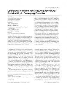
Prior beliefs about the parameters are given by the prior density 'prob(parameters)' and the likelihood of the sample data 'prob(dataparameters)' is called the sample likelihood. The product of these two densities defines the posterior density 'prob(parameters data)', that incorporates both prior beliefs and sample information into a revised and updated view of the model parameters, as depicted in figure 1.
Figure 1: The posterior density is a product of the prior density and the sample likelihood
Posterior
Likelihood
Prior
Parameter If prior beliefs are that all values of parameters are equally likely, this is the same as saying there is no prior information. The prior density is just the uniform density and the posterior density is just the same as the sample likelihood. But more generally the posterior density has a lower variance than both the prior density and the sample likelihood. The increased accuracy reflects the value of additional information, both subjective as encapsulated by prior beliefs and objective as represented in the sample likelihood.
Subjective beliefs may have a great influence on model parameter estimates if they are expressed with a high degree of confidence. Figure 2 shows two posterior densities based on the same likelihood. In figure 2a prior beliefs are rather uncertain, represented by the large variance of the © ISMA Centre, The Business School for Financial Markets
10
Discussion Papers in Finance: 2000-02
prior density. So the posterior density is close to the sample likelihood and prior beliefs have little influence on the parameter estimates. But in figure 2b, where prior beliefs are expressed with a high degree of confidence, the posterior density is much closer to the prior density and parameter estimates will be much influenced by subjective prior beliefs.
Figure 2: The posterior density for (a) uncertain prior beliefs and (b) confident prior beliefs
Posterior Prior Likelihood
Posterior
Likelihood
Prior
Parameter
Parameter
Of course, it is not just prior expectations that have an influence: the degree of confidence held in one's beliefs also has an effect. Bayesian analysis simply formalizes this notion: posterior densities take more or less account of objective sample information depending on the confidence of beliefs, as captured by the variance of prior densities. There is no single answer to the question of how much sample information to use and how confident prior beliefs should be. The only way one can tell which choices are best for the problem in hand is, as with any statistical model, to conduct a thorough back testing analysis.
Bayesian Belief Networks During the last few years there has been increasing interest in the use of causal networks to model operational risks, and in particular to use Bayesian belief networks (BBNs). Reasons for this surge of interest include: Ø
A BBN describes the factors that are thought to influence operational risk, thus providing explicit incentives for behavioural modifications;
© ISMA Centre, The Business School for Financial Markets
11
Discussion Papers in Finance: 2000-02 Ø
BBNs have the ability to perform scenario analysis to measure maximum operational loss, and to integrate operational risk with market and credit risk;
Ø
BBNs have applications to a wide variety of operational risks. Over and above the categories where available data enable the modelling of operational risk with standard statistical models, BBNs have applications to areas where data are more difficult to quantify, such as human risks;
Ø
Augmenting a BBN with decision nodes and utilities improves transparency for management decisions.
The basic structure of a BBN is a directed acyclic graph where nodes represent random variables and links represent causal influence. There is no unique BBN to represent any situation, unless it is extremely simple. Rather, a BBN should be regarded as the analyst's view of process flows, and how the various causal factors interact. In general, many different BBNs could be used to depict the same process.
A simple BBN that models the client services team of example 1 is shown in figure 3. The nodes 'Team', 'Market' and 'Client' represent random variables each with two possible outcomes, and the probability distribution on the outcomes is shown on the right of the figure. It is only necessary to specify the probability distribution of the two parent nodes (Team and Market) and the conditional probabilities for the Contract. The four conditional probabilities 'prob(winmarket = good and team = not satisfactory)' and so on, are shown below the Contract node. The network then calculates prob(win) = 68.75% and prob(lose) = 31.25%, using Bayes rule. The BBN may be used for scenario analyses. For example, if the contract is lost, what is the revised probability of the team being unsatisfactory? The bottom right box in figure 3 shows that the posterior probability that the team is unsatisfactory given that the contract has been lost is 52%, as already calculated in example 1.
© ISMA Centre, The Business School for Financial Markets
12
Discussion Papers in Finance: 2000-02
Figure 3: A simple BBN for the client services problem
More nodes and causal links should be added to the BBN until the analyst is reasonably confident of his or her prior beliefs about the parent nodes. So in the client services example, the factors that are thought to influence team performance, such as pay structure, appraisal methods, staff training and recruitment procedures can all be added as parent nodes to the Team node. But if a node has many parent nodes these conditional probabilities can be very difficult to determine because they correspond to high dimensional multi-variate distributions. A useful approach is to define a BBN so that every node has no more than two parent nodes. In this way the conditional probabilities correspond to bivariate distributions, which are easier for the analyst to visualize.
For the management of operational risks, a BBN may be augmented with decision nodes and utilities. In the simple example of client services, the decision about whether or not to restructure the team, and the costs associated with this decision are illustrated in figure 4. The node diagram in figure 4a depicts a dynamic decision process, where the decision about restructuring affects the team performance in the next period. The conditional probabilities (not shown) are such that a decision to restructure the team increases the chance of winning the contract in the next period.
In the initial state of the network, with the utilities and prior probabilities shown in the left column of figure 4b, there is a utility of 19.38 if the team is restructured at the end of the first
© ISMA Centre, The Business School for Financial Markets
13
Discussion Papers in Finance: 2000-02
period, but a utility of 20.33 if it is not restructured. So the optimal decision would be to leave the team is it is. However if the contract in the first period were lost (a scenario shown in the right column of figure 4b) the situation reverses, and it become more favorable to restructure the team. A similar scenario analysis shows that if the recommendation of the network is ignored and the team is not restructured, and if the contract in the second period is also lost, the utility from restructuring in the second period would be 1.79. The utility is 1.52 if the team were left unchanged, so again the network recommends a restructuring of the team.
Figure 4a: Architecture of a Bayesian decision network
© ISMA Centre, The Business School for Financial Markets
14
Discussion Papers in Finance: 2000-02
This example shows how a BBN may be augmented with decision variables to focus on operational management decision processes. Just one of many possible scenarios has been illustrated, and to explore more possibilities the interested reader is encouraged to replicate this example, or to construct a decision network more relevant to their own needs, using a BBN package.7
Figure 4b: Probabilities and utilities in a Bayesian decision network
7
There are several software packages for Bayesian networks that are freely downloadable from the Internet. Microsoft provides a free package for personal research only that is Excel compatible at www.research.microsoft.com/research.dtg/msbn/default.htm and a list of free (and other) Bayesian network software is on http.cs.berkeley.edu/~murphyk/Bayes/bnsoft.html © ISMA Centre, The Business School for Financial Markets
15
Discussion Papers in Finance: 2000-02
Application of a BBN to Modelling Settlement Loss This section presents a BBN model of the operational loss from settlement risk. This is the loss arising from interest foregone, fines imposed or borrowing costs as a result of a delay in settlement. It does not include the credit loss if the settlement delay is due to counterparty default, but it may include any legal or human costs incurred when settlement is delayed. Lack of space precludes attempting a complete specification of the type of network that a bank might use for settlement loss in practice.8 A complete process model of settlement failure would include client information, details of counterparty confirmations, valuation matching between front and back office, legal entity confirmation, trade capture, window dressing, remote booking and so forth.9 The model presented in figure 5 uses a much more simple macro perspective, but it is sufficient to illustrate the important points, viz. how BBNs: Ø
specify the causal factors that influence an operational loss distribution;
Ø
back test against historical loss event data to revise the network parameters;
Ø
employ scenario analysis to identify maximum operational loss.
Data from the trading book provide the probabilities for each node in figure 5. For example the probabilities assigned to the 'Country' node show that 70% of spot FX trades are in European currencies, and 20% of derivative securities trades are in Asia. Similarly the 'Delay' node shows that only 50% of over-the-counter trades in Asia experienced no delay, 0.6% of exchange traded European assets experienced five or more days delay in settlement, and so on. And the 'Notional' node shows that 35% of European FX trades were in deals in the 40-50$m bracket, but just 5% of trades in European securities fall into this bracket.
There are many conditional probabilities in the 'Loss' node even in this simplified model. The loss is calculated as a function L(m,t) of the notional m and the number of days delay t. This function depends on many things, including the settlement process (delivery vs payment, escrow, straightthrough, and so on), and whether legal and human costs are included in settlement loss. In the example the notional of a transaction is bucketed into 10$m brackets, and the loss distribution is given in round $000's. So for example the loss distribution in the initial state, shown in the left column in figure 5b, gives an expected loss of 274.4$ per transaction and a 99% tail loss of 4,763$ per transaction.
8 9
Such a model has been developed by Algorithmics Inc. (see www.algorithmics.com). Source: Personal communication with John Hedges, FSA London. © ISMA Centre, The Business School for Financial Markets
16
Discussion Papers in Finance: 2000-02
Figure 5a: Network architecture for settlement loss
© ISMA Centre, The Business School for Financial Markets
17
Discussion Papers in Finance: 2000-02
Obviously this picture of the settlements process is not unique. For example the analyst might wish to categorize trades not just by country and asset type, but also according to whether the trades were in derivatives or the underlying. In that case the architecture of the network should be amended by adding a causal link from the 'Product' node to the 'Notional' node. Alternative architectures could have the 'Country' node as a root node, or other nodes could be added such as the settlement process or the method for order processing. And most nodes in this example have been simplified to have only two states, so 'Country' can only be Europe or Asia, 'Asset' can be only foreign exchange or security, and so on. But the generalization of the network to more states in any of these variables is straightforward and the simple node structure given here is clear enough to illustrate the main ideas.
Which is the best of many possible specifications of a BBN for settlement loss will depend on the results of back tests. A number of different network architectures for modelling settlement loss could be tested. For each, the initial probabilities10 should be based on the current trading book, and the result of the network in this initial state could then be compared with the current settlement loss experienced. A basis for back testing is to compare the actual settlement loss that is recorded with the predicted loss, using a simple goodness-of-fit test. By performing back tests over suitable historic data, perhaps weekly during a one-year period, the best network design would be the one that gives the best diagnostic statistic in the goodness-of-fit test.
BBNs lend themselves very easily to scenario analysis. The operational risk manager can ask the question 'what is the expected settlement loss from over-the-counter trading in Asian FX futures'? The right column in figure 5b illustrates this scenario: per transaction the expected loss is 1,069.5$ and the 99% tail loss is 5,679$. Similarly the manager might ask 'what is the expected settlement loss from an FX trade in the 40-50$m bracket'? By setting probabilities of 1 on FX in the 'Product' node and on 40-50$m in the 'Notional' node, the answer is quickly calculated as 400.5$m. The interested reader can verify this is by replicating the network with one of the packages mentioned in footnote 8.
10
That is, the probabilities from the initial propagation of the network, before it is propagated again for scenario analysis. © ISMA Centre, The Business School for Financial Markets
18
Discussion Papers in Finance: 2000-02
Figure 5b: Scenario analysis for settlement loss
BBNs are not the only models that measure settlement loss; after all if historic data are available for back testing a network then they could be used to generate empirical settlement loss distributions. But BBNs improve transparency for internal management, not just because they identify the causal factors and how they inter-relate. BBNs lend themselves so easily to scenario analysis that operational risk managers can quickly identify the types of trades and operations where the settlement process is likely to present the greatest risk. Also by simulating scenarios on market risk factors such as interest rates and exchange rates, and credit risk factors such as credit ratings, managers can judge how operational risks are integrated with market and credit risks.
© ISMA Centre, The Business School for Financial Markets
19
Discussion Papers in Finance: 2000-02
Application of a BBN to Modelling Human Risk Finally, a simple network to model the human risk in transactions processing is described. The architecture shown in figure 6a uses the number of transactions processed per day as the key performance indictor. The node probabilities on the left of figure 6a are obtained by indicating the relevant manager, their pay scale, the recruitment process and the level of training of each person involved in transactions processing. To keep things simple the network illustrated has only binomial variables for the causal factors, but they could of course have many states, so for example there could be more than two possible managers, or certain causal variables such as pay could be continuous.
Figure 6a: BBN for number of transactions processed
The conditional probabilities for the key performance indicator node are calculated as follows. First assume that all conditional distributions are normal, and then estimate the average number of transactions processed per day over a period of time, and the standard deviation, for all people managed by Mr. A, on pay scale 1, recruited from agency X and having a certificate of training. Continuing in this way across all possibilities will give the data shown in the table below.
© ISMA Centre, The Business School for Financial Markets
20
Discussion Papers in Finance: 2000-02
The multivariate distribution of the number of transactions processed per day in the initial state of the network is the mixture of normals shown in figure 6b. Then a scenario analysis over the managers, pay, recruitment and training can be employed to see how this distribution changes as the states of these causal factors are changed.
Figure 6b: Multivariate density for the number of transactions processed
© ISMA Centre, The Business School for Financial Markets
21
Discussion Papers in Finance: 2000-02
Summary This paper has shown how Bayesian methods may be applied to measure a variety of operational risks, including those that are difficult to quantify such as human risks. BBNs improve transparency for efficient risk management, being based on causal flows in an operational process. A BBN depicts the analyst's view of the process, and so many different network architectures could be built for the same problem. Not only is the architectural design open to subjective choice, in some problems the data itself is very subjective.
However BBNs lend themselves to back testing, so it is possible to judge which is the 'best' network design and what are the most appropriate beliefs about non-quantifiable variables. BBNs also lend themselves very easily to scenario analysis, both over the causal factors of operational risks and over market and credit risk factors. In this way 'maximum operational loss' scenarios can be identified to help the operational risk manager focus on the important factors that influence operational risk, and the integration of operational risk measures with market and credit risk measures can be achieved.
References Alexander, C. (2000) 'Bayesian Methods for Measuring Operational Risks' ICBI Risk Management Report. Hoffman, D.G. Ed (1998) 'Operational Risk and Financial Institutions' (Risk Publications) ISDA/BBA/RMA survey report (February 2000) 'Operational Risk - The Next Frontier' available from www.isda.org Jensen, F.V. (1996) An Introduction to Bayesian Networks (Springer Verlag). Pearl, J. (1988) Probabilistic Reasoning in Intelligent Systems (Morgan Kaufmann)
© ISMA Centre, The Business School for Financial Markets
22