Bayesian Modelling of Multi-View Mammography
Nivea Ferreira Institute for Computing and Information Sciences - Radboud University Nijmegen Marina Velikova Department of Radiology - UMC - Radboud University Nijmegen Peter Lucas Institute for Computing and Information Sciences - Radboud University Nijmegen
Abstract Screening mammography is of a crucial value for the early detection of breast cancer. Computer-aided (CAD) systems are developed in order to given support to radiologists on the detection of breast lesions and correct interpretation of cancers. As images of each breast are usually taken from different projections, yielding multiple views of the same breast, accurate detection of abnormal findings requires comparison between those views. Usually CAD systems do not take this information into account, assuming that mammographic views are independent. We, on the other hand, introduce in this paper different aspects of breast cancer modelling by combining multiple mammographic views using Bayesian network theory. The models we propose are based on advanced raw image data analysis and domain knowledge of mammographic screening and have the aim to evaluate alternatives for improving lesion detection accuracy.
1. Introduction It is well recognised in the field of medicine that the screening of women (from a certain age) for breast cancer (BC) is one of the major pillars of the management of this disease. In particular, screening mammography has a crucial value in the course of early detection of breast cancer and is known to be decisive for a curative therapy. Appearing in the Proceedings of the ICML/UAI/COLT 2008 Workshop on Machine Learning for Health-Care Applications, Helsinki, Finland, 2008. Copyright 2008 by the author(s)/owner(s).
[email protected]
[email protected]
[email protected]
The description of the mammographic changes associated to breast cancer are inherently uncertain. For instance, a cirscumscribed lesion with spiculated (i. e., radiating) margin, irregular shape, average size of 1.5 cm and high density (i. e., it appears “whiter” on the mammogram than normal breast tissue) is a suspicious abnormality, that is likely, but not necessarily, cancer. Other changes such as (micro)calcifications, architectural distortion and asymmetry are described in similar fashion (Dronkers et al., 2002). Due to the diversity in nature, a cancerous finding is represented in different ways on mammograms and may, therefore, be difficult to observe. The identification of one abnormality might result, for instance, in having other abnormalities being overlooked, either in the same or in the other breast. When analysing mammograms the subtle changes, which are not always clearly or easily detectable, are the ones that bring concern. As a consequence, we often see radiologists’ misinterpretation of lesions, which are treated as being not suspicious enough for further examination. Computer-aided detection (CAD) systems have been developed as a supporting tool for radiologists, and many available classification methods have been explored in the hope that the performance of such systems would improve. Researchers in the area are now increasingly thinking that the explicit incorporation of domain knowledge is the way to make further progress. The design of a Bayesian network in the context of image analysis has particular implications with respect to the structure and content of that network; i. e., the understanding of the variables used, and the relation among those. This is seen as the major contribution of the present paper. The quality of the models developed is also experimentally evaluated. The paper is organised as follows. In the next sec-
Bayesian Modelling of Multi-View Mammography
tion we introduce terms and concepts from the area of screening mammography, and also Bayesian networks theory. In Section 3, relevant research work on computer-aided interpretation of screening mammograms is then reviewed. In Section 4 we give a description of the features which are relevant for the interpretation of mammograms, and introduce the models we have designed. Experimental results are subsequently presented in Section 5. Finally, in Section 6, final remarks and future work are provided.
(a)
(b)
Figure 1. A detected cancerous lesion (in circle) projected in (a) MLO view and (b) CC view.
2. Background 2.1. Screening Mammography Mammographic images are obtained from different projections, which are usually the mediolateral oblique (MLO) and craniocaudal (CC) positionings. CC views produce images of the breast from above, having the nipple on the center of the image, while MLO is a angled (approximmately 45-degree) projection, depicting the pectoral muscle. In the interpretation of mammograms, an area of interest is called a region of interest, or ROI for short. This region is characterised by means of features (e. g., size, density and location). Those features are used in the analysis of such images, and they may (or may not) suggest a certain level of suspiciousness for the presence (or development) of breast cancer. Furthermore, we denote as finding (lesion or abnormality) the corresponding regions of interest found in different views. That is, having observed a region in one view, we talk about correlating it to a (possible) region in the other view. An example is shown in Figure 1. Usually, a circumscribed lesion is defined as a threedimensional lesion that should, but need not, be observed in both views and is described in terms of its margin, shape, size and density. They represent a group of cells clustered together, appearing denser when compared to surrounding tissue. Considering both MLO and CC information is required in order to obtain an accurate detection of abnormal findings. This is what we explicitly represent in our models presented in Section 4. 2.2. The Single-View CAD System Computer-aided detection systems have as aim the increase of detection rate when analysing mammograms. The main idea is identifying features that are characteristics for breast cancer through pattern recognition techniques. As stated in (van Engeland, 2006) even though most CAD systems has the purpose of avoid-
ing detection errors, there can also help on improving interpretation of detected lesions - increasing radiologists’ performance. The CAD system that was used in this research (van Engeland, 2006; Timp, 2006), processes images by performing a number of steps: (i) segmentation of the mammogram into background area, breast and pectoral muscle (the latest only on the MLO view); (ii) initial detection of suspicious pixel-based locations; (iii) for each extracted region a number of continuousvalued features are then computed; and (iv ) each region is then classified as “normal” or “abnormal” based on the region features. A score for suspiciousness (or, likelihood) is computed and converted into false positive level (FPlevel), i. e., the average number of normal regions with the same or higher suspiciousness score. One characteristic of such systems is the ability to learn from data, which is specially relevant when a large amount of information is available. On the other hand, those systems are usually highly-dependent on the data samples and do not incorporate much background knowledge of the domain. 2.3. Bayesian Networks The differentiation between suspicious and nonsuspicious abnormalities of the breast as well as the association among various mammographic regions are difficult due to the inherent uncertainty in the breast cancer detection domain. As we show in this paper, probabilistic approaches, in special Bayesian networks, are potentially useful tools for modelling those problems. Here we briefly review BN technology. Let P be a joint probability distribution of the variables in U and let X, Y, Z be subsets of U . X and Y are conditionally independent given Z, denoted by X ⊥ ⊥ Y | Z, if for all x ∈ dom(X), y ∈ dom(Y ), z ∈ dom(Z), the following relationship holds: P (x | y, z) = P (x | z) whenever P (y, z) > 0
(1)
Bayesian Modelling of Multi-View Mammography
Note that dom(X) represents the domain of variable X. In short, we write Equation (1) as P (X | Y, Z) = P (X | Z). In certain cases, however, the conditional independence between X and Y may only hold for certain values z ∈ dom(Z), the so-called contexts. Hence, we have contextual independence of X and Y given context Z = z. Bayesian networks are defined as acyclic directed graphs with an associated joint probability distribution, where there is a 1–1 correspondence between nodes in the graph and random variables in the probability distribution that is factorised according to the structure of the graph. It is important to notice that under some conditions, the acyclic direct graph can be given a causal interpretation: nodes correspond to random variables from the modeled domain while arcs correspond to direct causal relationships between the variables (Pearl, 1988; Jensen & Nielsen, 2007).
However, even though these systems demonstrate good performance on distinguishing between true and false linking of regions, they do not provide evidence for improvement in the case interpretation. We want to be able not only to produce a coherent detection and linking of corresponding regions (in both views) but to assist on the interpretation whether, based on the information about the detected regions, a given case is to be considered as suspicious. In (Velikova et al., 2008) the same objective is pursued - meaning, the use of multiple views information to improve image interpretation. The BN model shown there combines the information from all the regions in MLO and CC, detected by the single-view CAD system, and obtain a single probabilistic measure for suspiciousness of a case. However, the BN framework used there, based on noisy-OR functions, differs greatly to the causal model, and its background knowledge emphasis, that we give in this work.
3. Related Work In the models presented in this paper, findings are taken as corresponding regions in two views. Through this modelling we design more realistic breast cancer domain models than it has been previously done. For instance, breast cancer models which use Bayesian networks theory, such as in (Kahn et al., 1997; Burnside et al., 2006), usually incorporate the characteristic features of breast cancer lesions (such as margin, size and shape). However, the specification of those are often based on the BI-RADS (BI-RADS, 1993) terms and definitions, once systems utilise radiologist’s interpretations of images in order to calculate breast cancer development risk (for a given case). It is then assumed that features are independent from one another and raw data analysis is not tackled. In terms of multi-view breast cancer detection, a number of approaches exist. Good et al. (Good et al., 1999) proposed a probabilistic model for correct matching of regions detected in both views. Van Engeland et al. develop in (van Engeland et al., 2006) a method for linking ROIs from different views, based on linear discriminant analysis classifier and a set of view-link features. The classifier computes a correspondence score for every possible region matching. This score is further used, as seen in (van Engeland & Karssemeijer, 2007), to recompute the level of suspisciouness of all initially detected regions1. In other words, making use of two-view information to improve the single-view CAD suspisciouness predictions. 1
Detection done by the single-view CAD system described in Section 2.2.
4. Mammography Bayesian Networks Incorporation of background knowledge from a domain into the design of a Bayesian network might improve the interpretation of data. However, it has been very difficult to prove that this is indeed the case. In particular, naive Bayesian classifier or the tree-augmented Bayesian classifier, have often yielded equal to superior performance (Domingos & Pazzani, 1997; Friedman et al., 1997). Here we have designed a multi-view causal model which incorporates image analysis knowledge, aiming to obtain an understandable domain description, in terms of the variables represented and the mechanisms under which those variables are related to one another. Together with this, we also have developed a naive Bayes model, which is simpler in terms of the independences assumed - but usually powerful with respect to classification accuracy. By examining both models, we intend to obtain a (preliminary) evaluation on the use of background knowledge in such domain. However, before presenting a detailed account on both models, we present below the features that are considered useful for the analysis of mammograms. 4.1. Mammographic Features Every mammmographic image corresponds to a breast and a particular view (MLO or CC). For each image we have the total number of annotated regions and the features description of each of those regions. In detail, the features used in our models are: loca-
Bayesian Modelling of Multi-View Mammography
tion - relative location of region (with radius of the breast), distance to skin, size or the area of the region, contrast, focal mass - describing the existence of a circumscribed lesion, spiculation - pattern of straight lines directed toward the center of a lesion (which is indicative for malignancy) and linear structure - indicating the presence of normal breast tissue pattern. Two other values computed by the single-view CAD system are also going to be considered as mammographic features in both multi-view causal and naive Bayes models, Pixel-based malignancy likelihood, and False-positive Level (FPLevel). We expect these values to be an extra indicative measure for the highly suspicious regions. Note that all mammographic features are continuousvalued variables. 4.2. Naive Bayesian Model A naive Bayesian (NB) classifier is a very popular special case of Bayesian networks. These network models have a central node, called the class node C, and nodes representing feature variables Fi , i = 1, . . . , n, n ≥ 1; the arcs going from the class node C to each of the feature nodes Fi (Jensen & Nielsen, 2007). The conditional independence that explains the adjective ‘naive’ determines that each feature Fi is conditionally independent of every other feature Fj , for j 6= i, given the class variable. In other words, P (Fi | C, Fj ) = P (Fi | C) The joint probability distribution underlying the model is: P (C, F1 , . . . , Fn ) = P (C)
n Y
probable hypothesis - a maximisation criterion. In this case, the classifier is defined by the function: NB(f1 , . . . , fn ) = argmax P (C = c) c
n Y
P (Fi = fi | C = c) (2)
i=1
In our particular case Finding is the discrete class variable and the considered features are the mammographic measures described in the previous section, available for both MLO and CC views. 4.3. Multi-View Causal Model
P (Fi | C),
i=1
and the conditional distribution over the class variable C can be expressed as P (C | F1 , . . . , Fn ) =
Figure 2. Causal model representing the domain of breast cancer detection on mammograms.
n Y 1 P (Fi | C), P (C) Z i=1
given a normalising factor Z. In many practical applications, parameter estimation for naive Bayes models uses the method of maximum likelihood estimates. Despite their naive design and apparently over-simplified assumptions, naive Bayes classifiers often demonstrate a good performance in many complex real-world situations. The naive Bayes classifier combines the above naive Bayesian network model with a decision rule (Domingos & Pazzani, 1997). A common rule is choosing most
Given that a region of interest is observed in a particular view, we aim to establish whether that represents a breast cancer finding. One way is to consider a classifier such as the naive Bayes model. Another is the next model, where features are not necessarily independent from each other. The causal model given in Figure 2 is an application of the general BN theory (seen in Sect. 2.3) on the breast cancer detection domain. The model is based on the literature on breast cancer detection on mammograms, such as (BI-RADS, 1993; Dronkers et al., 2002), and radiologists’ practice. The white boxes represented the features extracted from a mammogram (the same ones used in the NB model); and balloons represent non-observed discrete variables – capturing the combination of features from both views (such as Size and Spiculation) to the class variable Finding. Shades organize those hidden variables in different levels.
Bayesian Modelling of Multi-View Mammography
The meaning of discrete variables are as follows. Abnormal Density (AbnDens) represents an abnormal finding, not making any distinction between cirscumscribed lesion, architectural distortion or asymmetry three possible manifestations of an abnormality. Finding is a parent node of AbnDens. Through Abnormal Structure (AbnStruc) we capture the dependence between Spiculation (Spic) and Linear Texture (LinText). As in the domain, the presence of highly spiculated regions is expected to rule out the observation of linear texture. Formally speaking, Spic is independent of LinText given AbnStruc, Spic ⊥ ⊥ LinT ext | AbnStruc. Abnormal Density is characterized by a number of features whose values are derived as a overall measure of two indicators obtained from both MLO and CC views. According to the Bayesian modelling those features (Focal Mass, Abnormal Structure, Contrast and Size) are related to one another through AbnDens. Pixel-based malignancy likelihood (DLik) and Falsepositive Level are used as conditional variables to determine a priori the probability of having a finding. We represent Finding as a variable for which we seek inference. Clearly, as described above, in this model its descriptors are no longer all independent, in contrast to the naive Bayes approach. The labels used for the some of those discrete variables are as given in Table 1. Table 1. Variables used in the breast cancer causal model with their values.
Node Finding Abn. Density Size Contrast Spiculation Linear Texture
States true, false true, false small, medium, large low, high present, absent present, absent
taining 1,063 screening exams of which 383 are confirmed as cancerous by pathology reports. All exams contained both MLO and CC views. The total number of breasts is 2, 126. All cancerous breasts have a visible abnormality representing circumscribed lesion, architectural distortion, or asymmetry in at least one view. Lesion contours were marked by, or under supervision of, an experienced screening radiologist. Remember that the single-view CAD system processes the mammographic images, identifying regions of interest and, given the features for each of those, it computes the corresponding FPLevels. Therefore, for each exam, we obtain information referrent to the (at most) first 5 detected regions – sorted with respect to their FPLevel (lowest FPLevel first). In this dataset in particular, there were in total 10, 478 MLO regions and 10, 343 CC regions. Finally, every region from the MLO view was linked with every region in CC view, thus obtaining 51, 088 links in total. Each line of the dataset is then formed by the exam identification number, the identification numbers of the region in MLO and the region in CC (to which MLO region is assumed to be linked to), and the individual continuous features of each of those regions. Furthermore, the pathological information describes the nature of this link: a confirmed cancerous region is true positive (TP) either in MLO or CC, or both. If a true region in MLO is linked to the corresponding true region in CC (a TPTP link) then we have a finding. Any other type of link (i. e., TPFP, FPTP, FPFP - or, non-TPTP links) are not considered as finding. Despite the large number of region links we have in the data, only 581 represent a finding projected in the two views, i. e., a true link: a cancerous region in the MLO view and its corresponding region in the CC view. Both Bayesian networks were designed, trained and tested using the Bayes Net Toolbox for Matlab (Murphy, 2001). The parameter learning was done using the EM algorithm (Bilmes, 1998) in order to handle the missing values for the non-observable variables of the causal model.
5.1. Experimental Set-up
The evaluation of each network performance is done using two-fold cross validation: the dataset is split into two subsets with approximately equal number of observations (of non-TPTP links and TPTP ones). However, this is not done randomly: links which refer to the same exam are contained in the same subset. One subset is used as a training set and the other as test set, and then the other way around.
Both multi-view causal model and naive Bayes were implemented, and then evaluated using a data set con-
For all the continuous variables a normal (i. e., Gaussian) distribution was assumed. Most discrete-valued
Given data from both views and breasts, both naive Bayes and causal models “should” learn what describes (or not) a true linking of regions in general. This is what we show in detail in the next section.
5. Experiments and Results
Bayesian Modelling of Multi-View Mammography ROC curve per MLO view 1 0.9
True positive rate
variables assume a uniform (Dirichlet) distribution. However, the prior probabilities of Finding, for instance, were defined according to domain knowledge. The distribution of this variable given its parents FPlevel and DLik is presented in Table 5.1.
0.8
Causal model AUC: 0.747
0.7
Naive Bayes AUC: 0.725
0.6 0.5 0.4 0.3
Table 2. Prior probability distribution of Finding.
0.2 0.1
FPlevel n-susp n-susp susp susp
0
0
0.1
0.2
0.3
0.4
0.5
0.6
0.7
0.8
0.9
1
False positive rate
true 0.05 0.7 0.85 0.9
In words, we can say that a Finding is highly “false” (0.95 probability) if DLik and FPlevel measures indicate non-suspiciousness. Furthermore, FPlevel is a better indicator for the level of suspiciosness of a finding as it is based on the features of regions.
Figure 3. ROC analysis per MLO view ROC curve per CC view 1 0.9
True positive rate
DLik n-susp susp n-susp susp
Finding false 0.95 0.3 0.15 0.1
0.8
Causal model AUC: 0.759
0.7
Naive Bayes AUC: 0.732
0.6 0.5 0.4 0.3 0.2 0.1 0
0
0.1
0.2
0.3
0.4
0.5
0.6
0.7
0.8
0.9
1
False positive rate
5.2. Preliminary Results Based on the probabilities predicted by the multi-view causal and naive Bayes models, we take the maximum probability for Finding as a measure for suspiciousness for MLO, CC and the breast as a whole. Recall that we want to bring some interpretation to the analysis of mammographic features. The intuition is that the maximum (predicted) probability for a particular region (being linked to another region in a different view) would represent the best candidate true link. The maximum value among those values for a region would then be the best prediction for this region. We define analogously a measure for breast and case. The performance of both models is measured by Receiver Operating Characteristic (ROC) curve and corresponding Area Under the Curve (AUC) (Hanley & McNeil, 1982). Figures 3 and 4 present the classification outcome for both models. The results indicate an overall improvement in the discrimination between suspicious and non-suspicious views for both MLO and CC - when comparing the causal model to the naive Bayes. For MLO view, the increase in the true positive rate is mostly for false positive rates in the range (0.2, 0.7), whereas for CC view this range shifts to (0.1, 0.6). Furthermore, in terms of AUCs the detection rate for CC views is better than that for MLO views for both causal and naive Bayes models. This could, for instance, be explained by the fact that the region classification on MLO views is more complicated due to the breast positioning.
Figure 4. ROC analysis per CC view
While the view results are promising,from a radiologists’ point of view it is more important to look at the breast and case level performance. The breast probability in Figure 5 is the maximum probability among the probabilities of the regions in that breast. Overall we see that the causal model again performs somewhat better than naive Bayes on distinguishing between suspicious and non-suspicious breasts. Another interesting result is that the largest improvement is observed in the lower scale of the false positive rate (< 0.5). This means that the causal model is capable of detecting more suspicious breasts without increasing the misclassification of links. The final analysis is based on case level, seen in Figure 6, where the case probability is computed by taking the maximum out of the two breasts. The results demonstrate that modelling causal relationships might not only facilitate the interpretation of the predictions but also improve the classification. 5.3. Further analysis In our understanding, our causal model shows as a reasonable design of the interaction between the used mammographic features. The improvement on model’s performance shows that incorporating domain knowledge - through comprehensible description of the rela-
Bayesian Modelling of Multi-View Mammography
picious which have value greater than 0.9. For NB this value occurs for 13% of normal breasts. Looking at the cancerous breasts, the causal model does not assign to any of them a probability value (for being suspicious) which is less than 0.1, whereas NB does so in 17% of those breasts. If we broaden this probability range to being less than 0.3, the causal modal assigns such values to 7% of the cancerous breasts and NB to 33% of them. Finally, with respect to cases, the LogLik for the causal model and NB are 0.85 and 2.14, respectively. Thus, the former fits better the probability distribution at breast and case level than the latter.
ROC curve per breast 1
True positive rate
0.9 0.8
Causal model AUC: 0.741
0.7
Naive Bayes AUC: 0.715
0.6 0.5 0.4 0.3 0.2 0.1 0
0
0.1
0.2
0.3
0.4
0.5
0.6
0.7
0.8
0.9
1
False positive rate
Figure 5. ROC analysis per breast ROC curve per case 1
In other words, we feel encouraged to believe that incorporating background knowledge leads to a better classification performance, when compared to simpler models such as naive Bayes. However, further experiments are still necessary in order to obtain more conclusive results.
0.9
True positive rate
0.8 0.7
Causal model AUC: 0.637
0.6
Naive Bayes AUC: 0.594
0.5 0.4 0.3 0.2 0.1 0
0
0.1
0.2
0.3
0.4
0.5
0.6
0.7
0.8
0.9
1
False positive rate
Figure 6. ROC analysis per case
tion among variables as well as coherent probabilities associated to this representation - is a powerful tool on understanding and efficiently modelling the breast cancer domain. However, even though we can say that the causal model outperforms naive Bayes when considering the curves presented in the previous section, these improvements are often small (< 10% and usually < 5%). We then had a closer look at the quality of classification of both models, computing the log likelihood of the estimated probabilities for breast and case by: N 1 X LogLik = − ln P (Cn |En ), N n=1
(3)
where N is the number of the unit (i. e., 2, 126 for breast and 1, 063 for case), and Cn and En are the class value and the feature vector of the nth observation, respectively. The value of LogLik indicates how close the posterior probability distribution is to reality: when P (Cn |En ) = 1, LogLikn = 0; otherwise, LogLikn > 0. When computing the log likelihood for the breast, the value for the causal model is 0.73 whereas for naive Bayes it is 1.412 . In only 2% of the normal breasts the causal model estimates probabilities of being sus2 It is important to mention that in 33 normal breasts Naive Bayes predicts P (Breast = suspicious) = 1, which would characterise a log likelihood equal to infinity.
One of the changes that might help refining both models is having a separate class label for each of the different types of links – TPTP, TPFP, FPTP and FPFP. This way the nature of the link can be, more appropriately, used on interpreting the results in view, breast and case levels. The intuition is that a cancerous region should contribute to the interpretation of images (in those levels) even if visible only in one view.
6. Conclusions Our causal model establishes a clear relation between features extracted from the application of the singleview CAD system on mammograms, being a more intelligible model than the analysis provided by blackbox approaches (such as artificial neural networks). Current results show that our multi-view causal model increases classification performance when compared to the NB. This can be especially valuable when the comparison is made on breast and case levels, where the background knowledge is important for representing the dependences among relevant concepts - something neglected by our naive Bayes approach. That is, incorporating experts’ knowledge potentially improves the representation of the breast cancer domain not only qualitatively - as the model shows relevant correlation among variables - but also quantitatively - with better classification of cases, which is useful for decision support purposes. However, as 33 out of 1, 743 is a small percentage, we substitute those values by P (Breast = suspicious) = 0.999999999999999, yielding a comparison among models. Notice that in the causal model the maximum probability assigned to a normal breast is 0.96.
Bayesian Modelling of Multi-View Mammography
Regarding future work, we will perform more experiments and broaden our analysis in order to refine our causal model, aiming to obtain a more significant classification improvement (particularly for breast and case levels). For instance, in a more complex design we incorporate the relation between the two breasts of a patient, dropping the broadly used assumption that information concerning those are independent. We also understand, as showed in (Nielsen et al., 2007), that some domains cannot be properly captured by classifiers such as naive Bayes or tree-augmented networks. Exploring more refined classifiers - e. g., making use of contextual independence (explained in Sect. 2.3) - or even models obtained from standard structure learning approaches, will most probably contribute to a better evaluation. A systematic analysis of the impact of the used data in both models, other measures (than maximum probabilities) for breast and case levels, and different distributions for discrete and continuous variables also remain as relevant work.
Acknowledgments This research is being funded by the Netherlands Organisation for Scientic Research (NWO) under BRICKS/FOCUS grant number 642.066.605. We would also like to thank Nico Karssemeijer and Maurice Samulski, from the Department of Radiology of the University Medical Center of Nijmegen University, for valuable discussions and data provision.
References BI-RADS (1993). Breast imaging reporting and data system atlas (BI-RADS). Reston, VA: American College of Radiology. Bilmes, J. A. (1998). A gentle tutorial on EM algorithm and its application to parameter estimation for gaussian mixture and hidden markov models (Technical Report TR-97-021). U. C. Berkeley. Burnside, E. S., Rubin, D. L., Fine, J. P., Shachter, R. D., Sisney, G. A., & Leung, W. K. (2006). Bayesian network to predict breast cancer risk of mammographic microcalcifications and reduce number of benign biopsy results. Journal of Radiology, 240, 666–673. Domingos, P., & Pazzani, M. (1997). On the optimality of the simple Bayesian classifier under zero-one loss. Machine Learning, 29, 103–130. Dronkers, D. J., Hendriks, J. H. C. L., Holland, R., & Rosenbusch, G. (2002). The practice of mammog-
raphy: pathology, technique, interpretation, adjunct modalities. Thieme: Stuttgart, New York. Friedman, N., Geiger, D., & Goldszmidt, M. (1997). Bayesian network classifiers. Machine Learning, 29, 131–163. Good, W., Zheng, B., Chang, Y., Wang, X., Maitz, G., & Gur, D. (1999). Multi-image CAD employing features derived from ipsilateral mammographic views. Proceedings of SPIE, 3661, 474–485. Hanley, J. A., & McNeil, B. J. (1982). The meaning and use of the area under a receiver operating characteristic (ROC) curve. Radiology, 143, 29–36. Jensen, F., & Nielsen, T. (2007). Bayesian networks and decision graphs, second edition. New York: Springer. Kahn, C. E., Roberts, L. M., Shaffer, K. A., & Haddawy, P. (1997). Construction of a Bayesian network for mammographic diagnosis of breast cancer. Computers and Biology and Medicine, 27, 19–30. Murphy, K. (2001). The Bayes net toolbox for Matlab. Computing Science and Statistics, 33. Nielsen, J. D., Rum´ı, R., & Salmer´on, A. (2007). Supervised classification using probabilistic decision graphs. Preprint submitted to Elsevier. Pearl, J. (1988). Probabilistic Reasoning in Intelligent Systems: Networks of Plausible Inference. San Francisco, CA: Morgan Kauffman. Timp, S. (2006). Analysis of temporal mammogram pairs to detect and characterise mass lesions. Doctoral dissertation, Radboud University Nijmegen. van Engeland, S. (2006). Detection of mass lesions in mammograms by using multiple views. Doctoral dissertation, Radboud University Nijmegen. van Engeland, S., & Karssemeijer, N. (2007). Combining two mammographic projections in a computer aided mass detection method. Medical Physics, 34, 898–905. van Engeland, S., Timp, S., & Karssemeijer, N. (2006). Finding corresponding regions of interest in mediolateral oblique and craniocaudal mammographic views. Medical Physics, 33, 3203–3212. Velikova, M., Lucas, P., Karssemeijer, N., Ferreira, N., & Samulski, M. (2008). A decision support system for breast cancer detection in screening programs. Proceedings of Prestigious Applications of Intelligent Systems (PAIS’08). To appear.