MovieLens-dataset, we can inspect its merits both qualitatively and quantitatively. Qualitatively, we find that ..... It's a Wonderful Life. 2. Raiders of the Lost Ark. 3.
i
67
Bayesian Networks for Collaborative Filtering Helge Langseth
Department of Computer and Information Science Norwegian University of Science and Technology NO-7491 Trondheim, Norway
Abstract In this paper we will present the basic properties of Bayesian network models, and discuss why this modelling framework is well suited for an application in collaborative filtering. We will then describe a new collaborative filtering model, which is built using a Bayesian network. By examining how the model operates on the well-known MovieLens-dataset, we can inspect its merits both qualitatively and quantitatively. Qualitatively, we find that the proposed model extracts and organises information about the relevant items in a well-defined way; quantitatively we find that the model’s recommendations appear to be better than those, which current state-of-the-art systems have to offer.
1
Collaborative filtering
When getting information about what book to read next or what movie to go to, we often rely on “word of mouth”: Friends and people we know tell us what they like, and if we believe their taste in books (or movies) is similar to ours, we may take their advise into account when trying to prioritise among the vast number of titles to choose from. The philosophy of a recommender system based on collaborative filtering (CF) takes the concept of “friends” one step further: Instead of relying on a select group of people and their reading lists, a CF system bases its suggestions on the collective ratings of the (possibly thousands of) users of a website. Based on these users’ preferences, typically represented by a matrix of ratings, a CF system will typically group its users into “communities” of users having similar taste, or group items into “categories” of items that tend to be liked by the same people. After grouping the users or items, a CF system will propose that a given user considers items that other members of that user’s community have shown an interest in, or which fall into the same category as other items liked by the user. In this paper we propose a probabilistic graphical model (represented by a linear Gaussian Bayesian network) for collaborative filtering. The model explicitly includes all users and items simultaneously in the model, and can therefore also be seen as a relational model combining both an item perspective and a user perspective. The generative properties of the model support a natural model interpretation. This paper was presented at NAIS-2009; see http://events.idi.ntnu.no/nais2009/.
i
i
i
i
68
2
H. Langseth
Bayesian networks
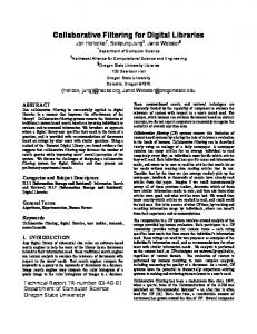
A Bayesian Network (BN) is a compact representation of a multivariate statistical distribution function [26, 5, 14]. A BN encodes the probability density function governing a set of random variables {X1 , . . . , Xn } by specifying a set of conditional independence statements together with a set of conditional probability functions. More specifically, a BN consists of a qualitative part, a directed acyclic graph where the nodes mirror the random variables Xi , and a quantitative part, the set of conditional probability functions. An example of a BN over the variables {X1 , . . . , X5 } is shown in Figure 1, only the qualitative part is given. We call the nodes with outgoing edges pointing into a specific node the parents of that node, and say that Xj is a descendant of Xi if and only if there exists a directed path from Xi to Xj in the graph. In Figure 1, X1 and X2 are the parents of X3 , written pa (X3 ) = {X1 , X2 } for short. Furthermore, pa (X4 ) = {X3 } and since there are no directed path from X4 to any of the other nodes, the descendants of X4 are given by the empty set and, accordingly, its non-descendants are {X1 , X2 , X3 , X5 }. The edges of the graph represents the assertion that a variable is conditionally independent of its non-descendants in the graph given its parents in the same graph; other conditional independence statements can be read off the graph by using the rules of d-separation [26]. The graph in Figure 1 does for instance assert that for all distributions compatible with it, we have that X4 is conditionally independent of {X1 , X2 , X5 } when conditioned on {X3 }. X1 X2
X3
X4
X5 Figure 1: An example BN over the nodes {X1 , . . . , X5 }. Only the qualitative part of the BN is shown. When it comes to the quantitative part, each variable is described by the conditional probability function of that variable given the parents in the graph, i.e., the collection of conditional probability functions {f (xi |pa (xi ))}ni=1 is required. The underlying assumptions of conditional independence encoded in the graph allow us to calculate the joint probability function as f (x1 , , . . . , xn ) =
n Y i=1
f (xi |pa (xi )).
(1)
Some of the main reasons why Bayesian networks have become widely used are (in the view of the author): Efficient calculation scheme: Efficient algorithms for calculating arbitrary marginal distributions, say, f (xi , xj , xk ) as well as conditional distributions, say, f (xi , xj |xk , xℓ ), make BNs well suited for modelling complex systems. Models over thousands of variables are not uncommon.
i
i
i
i
Bayesian Networks for Collaborative Filtering
69
Intuitive representation: The qualitative part (the graph) has an intuitive interpretation as a model of causal influence. Although this interpretation is not necessarily entirely correct, it is helpful when the BN structure is to be elicited from experts. Furthermore, it can also be defended if some additional assumptions are made [27]. To elicit the quantitative part from experts, one must acquire all conditional independencies (f (xi |pa (xi )) for i = 1, . . . , n in Equation (1)), and once again the causal interpretation can come in as a handy tool. Model fitting: Methods for estimating the quantitative part of the BN from data date back to the work of the early nineties [30], see also [19]. A method for estimating the qualitative part from data was pioneered by [4], and is still an active research area. Compact representation: Through its factorized representation (Equation (1)), the BN attempts to represent the multi-dimensional distribution in a costefficient manner. Expressive representation: A BN can represent or approximate any probability density function. The BN representation has traditionally been limited to only handle discrete distributions in addition to a particular class of hybrid distributions, the so-called conditional Gaussian distributions [20]. Recently, a framework for approximating any hybrid distribution arbitrarily well by employing mixtures of truncated exponential (MTE) distributions [25]. They also show how the BN framework’s efficient calculation scheme can be extended to handle the MTE distributions.
3
Probabilistic models for collaborative filtering
Probabilistic graphical models for collaborative filtering include general unconstrained models such as standard Bayesian networks [2] and dependency networks [9]. These types of models have, however, received only modest attention in the collaborative filtering community, mainly due to the complexity issues involved in learning these models from data. Instead research has focused on models, which explicitly incorporate certain independence and generative assumptions about the domain being modelled. The most simple probabilistic model for collaborative filtering is the multinomial mixture model [2], where like-minded users are clustered together in the same user classes, and given a user class a user’s ratings are assumed independent (i.e., the model basically corresponds to a naive Bayes model [8]). The independence assumptions underlying the multinomial mixture model do usually not hold, and has been studied extensively, in particular w.r.t. models targeted towards classification [17, 7]. However, for collaborative filtering the model has mainly been analysed w.r.t. its generative properties: The multinomial mixture model assumes that all users have the same prior probability distribution over the user classes, and given that a user is assigned to a certain class that class is used to predict the ratings for all items. The aspect model [13, 11, 12] addresses some of the inherent limitations of the mixture model by allowing users to have different prior distributions over the user classes. This idea is further pursued by [22] who introduces the user rating profile
i
i
i
i
70
H. Langseth
(URP) model that expands on the generative semantics of the aspect model, and allows different latent classes to be associated with different item ratings. The URP model shares the same computational difficulties as the latent Dirichlet allocation model [1], and relies on advanced approximate methods [28] for inference and learning. This model has been further explored by [28] who extend the latent model structure to cover both users and items. For a comparison and discussion on alternative models, including the aspect model and the flexible mixture model [29], see [15].
4
Our proposed model
In this section we will describe our collaborative filtering model, but first we need to introduce some notation. We will denote the matrix of ratings by R, which is of size #U × #M; #U is the number of users and #M is the number of movies that are rated. R is sparsely filled, meaning that it (to a large degree) contains missing values. The observed ratings are either realisations of ordinal variables (discrete variables with ordered states, e.g., “Bad”, “Medium”, “Good”) or real numbers. In the following we will consider only continuous ratings (ratings given as ordinal variables are hence assumed to have been translated into a numeric scale). We will use p as the index of an arbitrary person using the system, i is the index of an item that can be rated, and Rp,i is therefore the rating that person p gives item i. Finally, we let r denote all observed ratings (the part of R that is not missing). When working in model-based CF, we search for a representation of r based on model parameters θ, i.e., we assume the existence of a function g(·) s.t. r p,i = g(θ, p, i) for all the observed ratings. By the inductive learning principle we will predict the rating a person p′ gives to item i′ , r p′ ,i′ , as g(θ, p′ , i′ ). Often, g(·) will be based on a statistical model of the conditional distribution of Rp,i|{r, θ}, and the prediction is then either the expected value or the median value of that conditional distribution. As indicated above, most recommender systems are based on a clustering of either users or items. Unfortunately, by only considering one of these two perspectives one may potentially leave out important information, which could otherwise have improved the performance of the system, in particular when data is scarce. This observation is exploited in the following. Furthermore, our model will use latent variables to describe users and items abstractly as real vectors. We will use the model to consider all users and all items simultaneously. Let M i be the latent variables representing item i, and assume a priori that M i ∼ N (0, I), for 1 ≤ i ≤ #M. Similarly, for users we assume the existence of the latent variables U p representing user p, and choose U p ∼ N (0, I), for 1 ≤ p ≤ #U. The final model is now build by assuming that there exists a linear mapping from the space describing users and items to the numerical rating scale: Rp,i |{M i = mi , U p = up } = v Tp mi + wi iT up + φp + ψi + ǫ.
(2)
In Equation (2) we have introduced v p and w i , which are real vectors of “weights” taking the abstract item and user description, respectively, and map that into a numeric value. Furthermore, we introduce the constants φp and ψi , which can be interpreted as representing the average rating of user p and the average rating of item i (after compensating for the user average), respectively. Finally, ǫ represents “sensor noise”, i.e., the variation in the ratings the model cannot explain, and we will
i
i
i
i
71
Bayesian Networks for Collaborative Filtering U1 w3
w2
w1 R1,1
R1,2 v1
R1,3 v1
v1 M2
M1 v2
M3
v2
v2
R2,2
R2,1 w1
R2,3 w2 w3 U2
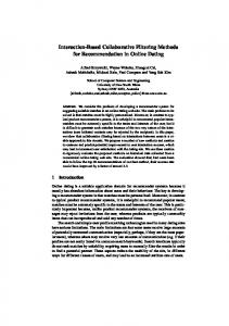
Figure 2: The full statistical model for collaborative filtering; this model has #M = 3 and #U = 2. assume that ǫ ∼ N (0, σ 2 ) for some fixed variance σ 2 . Note that we have the same number of latent variables for all users (i.e., |U o | = |U p |) and for all movies (i.e., |M r | = |M i |). Note that Equation (2) implicitly defines the full joint distribution over all ratings in the domain simultaneously, and the model is shown as a BN in Figure 2 for the special case of #U = 2 users and #M = 3 items. When learning the model, we need to find the number of latent variables to describe both users and items (the model structure) as well as learning the parameters for the chosen model structure. In our initial application of the model, the model structure is learned based on a greedy search. For a fixed model structure, the parameters in the model are learned using the EM algorithm [6].
5
Testing the model
To get additional insight into the model, it may be informative to analyse a model learned for a particular dataset. To this end, we learned a model for the MovieLens dataset [10] with three latent variables for each movie and one latent variable for each user, i.e., (|M | = 3 and |U | = 1). If we start off by considering the latent variables for the movies, then these variables can be interpreted as abstract representations of the movies. That is, for movie i we have a Gaussian distribution over ℜq (assuming |M i | = q), and ˆ i = E(M i |r) can therefore be considered a point estimate representation of movie m i. With this interpretation we hypothesise that if the point estimates of two movies are close in latent space, then they have the same abstract representation, and they should therefore be similar (i.e., have similar rating patterns). To test this hypothesis we determined the movies that are close to Star Wars (1977) and Three ˆ i and m ˆ j we used the Colours: Blue (1993).1 As distance measure for two movies m Mahalanobis distance to account for the correlation between the latent variables: ˆ m ˆ i, m ˆ j ) = (m ˆi−m ˆ j )T Q( ˆi−m ˆ j ), distM (m 1
i
In the analyses below, we only considered movies with at least 50 ratings.
i
i
i
72
H. Langseth 1. 2. 3. 4. 5. 6. 7. 8. 9. 10.
The Empire Strikes Back The Princess Bride Star trek II Return of the Jedi Raiders of the Lost Ark Star Trek IV Private Parts Star Trek VI Mystery Science Theatre 3000 Men in Black
1. 2. 3. 4. 5. 6. 7. 8. 9. 10.
Welcome to the Dollhouse Heavenly Creatures Three Colours: White Wings of Desire Everyone Says I Love You Muriel’s Wedding Dead Man Walking The Nightmare Before Christmas Boogie Nights To Die For
Table 1: The 10 movies closest to Star Wars and Three Colours: Blue, respectively. 1. 2. 3. 4. 5. 6. 7. 8. 9. 10.
Lost Highway Crash White Squall The First Wives Club Four Rooms The Unbearable Lightness of Being I Know What You Did Last Summer Angels and Insects Breaking the Waves Jane Eyre
1. 2. 3. 4. 5. 6. 7. 8. 9. 10.
Star Trek II The Empire Strikes Back Return of the Jedi Die Hard: With a Vengeance Raiders of the Lost Ark Star Wars Independence Day True Lies Star Trek IV Twister
Table 2: The 10 movies furthest away from Star Wars and Three Colours: Blue, respectively.
ˆ is the empirical precision matrix for the latent variables calculated from where Q the point estimates of the movies in the dataset. Star Wars is a sci.-fi./action movie with sequels The Empire Strikes Back and Return of the Jedi, so we would hope to see these movies, as well as other sci.-fi. movies, to be named “close” to Star Wars. On the other hand, Three Colours: Blue is a drama, and is the first in a trilogy of movies that also includes Three Colours: Red and Three Colours: White. The results are shown in Table 1.2 Out of the 10 movies closest to Star Wars, 7 are movies that the author believes are well classified as “similar to Star Wars”. The Princess Bride and Raiders of the Lost Ark are somewhat related in the sense that they are adventure movies, but Private Parts does not seem to fit in that well; we see a similar pattern for the movies closets to Three Colours: Blue. Considering that there are 1683 movies in the database we find this quite satisfactory. With the specified distance measure we are also able to find the movies furthest away from Star Wars and Three Colours: Blue. The results are shown in Table 2, where we find that the movies furthest away from Star Wars are primarily dramas and the movies furthest away from Three Colours: Blue are mainly action and sci.-fi. movies. One may also attempt to investigate whether the latent variables have a semantic interpretation. For this analysis we selected the movies with smallest and highest values along each of the three dimensions in the latent space. The results can be 2 Although not part of the table, we would like to note that Three Colours: Red comes in at rank 11 relative to Three Colours: Blue.
i
i
i
i
73
Bayesian Networks for Collaborative Filtering 1. 2. 3. 4. 5. 6. 7. 8. 9. 10.
Ace Ventura: Pet Detective A Nightmare on Elm Street Die Hard: With a Vengeance True Lies Twister Independence Day Die Hard 2 Top Gun Con Air Happy Gilmore
1. 2. 3. 4. 5. 6. 7. 8. 9. 10.
Angels and Insects Big Night Breaking the Waves Il Postino Three Colours: Blue The Crying Game Breakfast at Tiffany’s Cold Comfort Farm Harold and Maude Muriel’s Wedding
Table 3: The 10 movies with lowest and highest values in the first dimension in the latent space. Semantically, this dimension may be interpreted as to what extend the movie appeals to a teenage audience. 1. 2. 3. 4. 5. 6. 7. 8. 9. 10.
The Cook the Thief His Wife and Her Lover Mystery Science Theatre 3000: The Movie The City of Lost Children Delicatessen Army of Darkness Brazil Star Wars Star Trek II The Empire Strikes Back This Is Spinal Tap
1. 2. 3. 4. 5. 6. 7. 8. 9. 10.
The First Wives Club White Squall The Preacher’s Wife Dirty Dancing The Crucible Jane Eyre Crash Pretty Woman The Mirror Has Two Faces Little Women
Table 4: The 10 movies with lowest and highest values in the second dimension in the latent space. A semantic interpretation might be that this dimension represent to what extend the movie appeals to a male/female audience.
seen in Table 3–5. Based on the listed movies, one possible semantic interpretation might be that the first dimension encodes to what extend the movie would appeal to a teenage audience, the second dimension represent whether the movie appeals to a male/female audience, and the third dimension might represent whether the movie is a classic. Next, we consider the parameter ψi . Recall that this parameter is intended to represent the average rating of item i (after adjusting for the user types that has rated the movie), and ψi may therefore be thought of as representing the quality of an item. For illustration, we ordered the movies based on the estimated ψ-values. The result is shown in Table 6, where each movie’s position on the Internet Movie Database’s (IMDB’s) list of top 250 movies are given as reference.3 Note that our model also picked out three “Wallace and Gromit” movies as contenders for the top-ten list. These movies are either short-movies or a compilation of such, and do therefore not qualify for the IMDB top 250-list. We have therefore removed them from the results in Table 6 for ease of comparison. Note also that our dataset only contains movies released in 1998 or before, which explains why e.g. “The Dark Knight” (IMDB 8) and the “The Lord of the Rings” series (IMDB 13, 21, and 34) are not on our list. 3
i
http://www.imdb.com
i
i
i
74
H. Langseth 1. 2. 3. 4. 5. 6. 7. 8. 9. 10.
It’s a Wonderful Life Raiders of the Lost Ark Sleepless in Seattle E.T. the Extra-Terrestrial The Empire Strikes Back Singin’ in the Rain Dave The Firm Mary Poppins Dirty Dancing
1. 2. 3. 4. 5. 6. 7. 8. 9. 10.
Lost Highway Beavis and Butt-head Do America Event Horizon Four Rooms Natural Born Killers The Celluloid Closet Boogie Nights Koyaanisqatsi Crash The Ice Storm
Table 5: The 10 movies with lowest and highest values in the third dimension in the latent space. Semantically, this dimension may be interpreted as to what extend the movie is consider a classic. The IMDB Top 250 list is obviously not an objective truth, but we compare our results to it because the IMDB has a much higher number of ratings than the MovieLens dataset, and may therefore offer a more robust ranking. For comparison, we found that simply ordering the movies by their average rating did not give convincing results; none of the 10 movies that are top-ranked following this scheme are among the 250 movies in the “IMDB Top 250”-listing. We believe the reasons for this are twofold: i) the sparsity of the data; items with few ratings may get “extreme” averages, ii) simply talking averages disregards the underlying differences between users: Some are “happy” and others are “grumpy”. The fact that a “happy” user has seen movie i1 and a “grumpy” one has seen i2 does not mean that movie i1 is better than i2 (even though it may get a better rating). Finally, the merits of our CF system was assessed quantitatively. Again, we used the MovieLens dataset, and in particular utilised that this set has been divided into five cross-validation sets already. Depending on model structure, we obtained results (calculated as MAE, mean absolute error [23]) in the area 0.685 – 0.695, with the the best result found using |M | = 2 and |U | = 1. It is difficult to find results in the scientific literature that is directly comparable to ours, mainly because the experimental setting is different. Many researchers using the MovieLens dataset have made their own training and test sets without further documentation. However, the reported MAE values are typically about 0.73 – 0.74 [10, 21, 24, 16, 3]. 1. 2. 3. 4. 5. 6. 7. 8. 9. 10.
The Shawshank Redemption Schindler’s List Star Wars Casablanca The Usual Suspects Rear Window Raiders of the Lost Ark The Silence of the Lambs One Flew Over the Cuckoo’s Nest 12 Angry Men
IMDB: IMDB: IMDB: IMDB: IMDB: IMDB: IMDB: IMDB: IMDB: IMDB:
1 6 12 11 22 16 18 24 8 7
Table 6: The 10 “best” movies, i.e., the movies with the highest ψi value.
i
i
i
i
Bayesian Networks for Collaborative Filtering
6
75
Conclusions
This paper presents a BN model for collaborative filtering. The model offers a reasonable qualitative interpretation, and has been shown to provide good recommendations when measured using the mean absolute error. We are currently extending this model in a number of directions: i) Integrating the rating-information with content-information to improve the ratings; ii) looking into issues regarding computational complexity; iii) taking the CF models into new domains (like applications for tourists).
Acknowledgements The work presented here is joint with Thomas D. Nielsen at Aalborg University. An extended version of this paper is available as a Technical Report from Aalborg University [18].
References [1] David M. Blei, Andrew Y. Ng, Michael I. Jordan, and John Lafferty. Latent Dirichlet allocation. Journal of Machine Learning Research, 3:2003, 2003. [2] Jack S. Breese, David Heckerman, and Carl Kadie. Empirical analysis of predictive algorithms for collaborative filtering. In Proceedings of the Fourteenth Conference on Uncertainty in Artificial Intelligence, pages 43–52. Morgan Kaufmann Publishers, 1998. [3] J. Chen and J. Yin. Recommendation based on influence sets. In Proceedings of the Workshop on Web Mining and Web Usage Analysis, 2006. [4] Gregory F. Cooper and Edward Herskovits. A Bayesian method for the induction of probabilistic networks from data. Machine Learning, 9:309–347, 1992. [5] Robert G. Cowell, Alexander Philip Dawid, Steffen L. Lauritzen, and David J. Spiegelhalter. Probabilistic Networks and Expert Systems. Statistics for Engineering and Information Sciences. Springer-Verlag, New York, NY, 1999. [6] Arthur P. Dempster, Nan M. Laird, and Donald B. Rubin. Maximum likelihood from incomplete data via the EM algorithm. Journal of the Royal Statistical Society, Series B, 39:1–38, 1977. [7] Pedro Domingos and Michael Pazzani. On the optimality of the simple Bayesian classifier under zero-one loss. Machine Learning, 29(2–3):103–130, 1997. [8] Richar O. Duda and Peter E. Hart. Pattern Classification and Scene Analysis. John Wiley & Sons, New York, 1973. [9] David Heckerman, David Chickering, Chris Meek, Robert Rounthwaite, and Carl Kadie. Dependency networks for inference, collaborative filtering and data visualization. Journal of Machine Learning Research, 1:49–75, 2000.
i
i
i
i
76
H. Langseth
[10] Jon Herlocker, Joseph Konstan, Al Borchers, and John Riedl. An algorithmic framework for performing collaborative filtering. In Proceedings of the ACM 1999 Conference on Research and Development in Information Retrieval, pages 230–237, 1999. [11] Thomas Hofmann. Learning what people (don’t) want. In Proceedings of the Twelfth European Conference on Machine Learning, pages 214–225, London, UK, 2001. Springer-Verlag. [12] Thomas Hofmann. Latent semantic models for collaborative filtering. ACM Transactions on Information Systems, 22(1):89–115, 2004. [13] Thomas Hofmann Jan and Puzicha. Latent class models for collaborative filtering. In Proceedings of the Sixteenth International Joint Conference on Artificial Intelligence, pages 688–693, San Francisco, CA, USA, 1999. Morgan Kaufmann Publishers. [14] Finn V. Jensen and Thomas D. Nielsen. Bayesian Networks and Decision Graphs. Springer-Verlag, Berlin, Germany, 2007. [15] Rong Jin, Lao Si, and Chengxiang Zhai. A study of mixture models for collaborative filtering. Information Retrieval, 9(3):357–382, 2006. [16] Dohyun Kim and Bong-Jin Yum. Collaborative filtering based on iterative principal component analysis. Expert Systems with Applications, 28(4):823 – 830, 2005. [17] Helge Langseth and Thomas D. Nielsen. Latent classification models. Machine Learning, 59(3):237–265, 2005. [18] Helge Langseth and Thomas D. Nielsen. A latent model for collaborative filtering. Technical Report 09-003, Department of Computer Science, Aalborg University, Denmark, 2009. [19] Steffen L. Lauritzen. The EM-algorithm for graphical association models with missing data. Computational Statistics and Data Analysis, 19:191–201, 1995. [20] Steffen L. Lauritzen and Nanny Wermuth. Graphical models for associations between variables, some of which are quantitative and some qualitative. The Annals of Statistics, 17:31–57, 1989. [21] Qing Li and Byeong Man Kim. Clustering approach for hybrid recommender system. In WI ’03: Proceedings of the 2003 IEEE/WIC International Conference on Web Intelligence, pages 33–38, Washington, DC, USA, 2003. IEEE Computer Society. [22] Benjamin Marlin. Modeling user rating profiles for collaborative filtering. In Advances in Neural Information Processing Systems 15, pages 627–634. The MIT Press, 2003. [23] Benjamin Marlin. Collaborative filtering: A machine learning perspective, 2004. Master of Science Thesis, Graduate Department of Computer Science, University of Toronto.
i
i
i
i
Bayesian Networks for Collaborative Filtering
77
[24] Bamshad Mobasher, Xin Jin, and Yanzan Zhou. Semantically enhanced collaborative filtering on the web. In Web Mining: From Web to Semantic Web, First European Web Mining Forum, EMWF 2003, number 3209 in Lecture Notes in Computer Science, pages 57–76, 2003. [25] Serafín Moral, Rafael Rumí, and Antonio Salmerón. Mixtures of truncated exponentials in hybrid Bayesian networks. In Sixth European Conference on Symbolic and Quantitative Approaches to Reasoning with Uncertainty, volume 2143 of Lecture Notes in Artificial Intelligence, pages 145–167. Springer-Verlag, Berlin, Germany, 2001. [26] Judea Pearl. Probabilistic Reasoning in Intelligent Systems: Networks of Plausible Inference. Morgan Kaufmann Publishers, San Mateo, CA., 1988. [27] Judea Pearl. Causality – Models, Reasoning, and Inference. University Press, Cambridge, UK, 2000.
Cambridge
[28] Eerika Savia, Kai Puolamäki, Janne Sinkkonen, and Samuel Kaski. Two-way latent grouping model for user preference prediction. In Proceedings of the Twenty-first Conference on Uncertainty in Artificial Intelligence, pages 518– 525, 2005. [29] Luo Si and Rong Jin. Flexible mixture model for collaborative filtering. In Proceedings of the Twentieth International Conference on Machine Learning, pages 704–711. National Conference on Artificial Intelligence, 2003. [30] David J. Spiegelhalter and Steffen L. Lauritzen. Sequential updating of conditional probabilities on directed graphical structures. Networks, 20:579– 605, 1990.
i
i
i
i
78
i
i
i