Bayesian Ordinal Aggregation of Peer Assessments: A Case Study on

Bayesian Ordinal Aggregation of Peer Assessments: A Case Study on KDD 2015 Thorsten Joachims1 and Karthik Raman1 Cornell University, Ithaca NY 14853, USA

Abstract. Peer assessment is the most common approach to evaluating scientific work, and it is also gaining popularity for scaling evaluation of student work in large and distributed classes. The key idea is that each peer reviewer or grader rates a relatively small subset of the items, and that some method of manual, semiautomatic, or fully-automatic aggregation of all assessments defines the eventual rating of all items – the grade in peer grading, or whether to accept or reject a scientific manuscript. In this paper, we explore in how far a Bayesian Ordinal Peer Assessment (BOPA) method can provide additional decision support when making acceptance/rejection decisions for a scientific conference. Using data from the 2015 ACM Conference on Knowledge Discovery and Data Mining (KDD), where this system was deployed, we discuss the potential merit of the BOPA approach compared to conventional decision support offered by the Microsoft Conference Management System (CMT). Keywords: Peer Review, Peer Grading, Ordinal Feedback, Rank Aggregation

1

Introduction

Scientific conferences and large university courses both share the problem of evaluating large sets of items (e.g. scientific papers, project reports), where the quality of each item is difficult to evaluate automatically. A common approach is to use peer reviewing, where each reviewer assesses the quality of a small subset of the items. In such assessments, reviewers are typically asked to assign numeric scores regarding aspects and overall quality of the item, justifying each score with a written explanation. While this approach scales well with the number of items and allows complex criteria under which to evaluate quality, the key problems lies in aggregating the scores of a large number of reviewers into a coherent assessment of the items. For scientific conferences, the final assessment comes down to the decision of whether to accept or reject a paper. The most widely used approach for aggregating reviewer scores into an acceptance decisions relies on a hierarchy of reviewers, meta-reviewers, and program chairs. This is also the approach taken at the 2015 ACM Conference on Knowledge Discovery and Data Mining (KDD), which will server as a case study in this paper. Each of the reviewers assessed a small subset of all submissions, providing an average of 3.9 reviews per paper. Based on these reviews, meta-reviewers were then asked to make acceptance recommendations for their subset of papers. The program chairs made the final acceptance decisions based on the meta-reviewers’ recommendations, oversaw the process, and intervened in the reviewing process where necessary.

2

Fig. 1. Information provided to the meta-reviewers and program chairs for three example papers. In the posterior marginal rank distributions at the right of each panel, the x-axis shows the rank of the paper and the y-axis shows the probability of the paper placing at this rank. The plots also show posterior mean and median of the marginal distribution.

Under this decision making approach, both the meta-reviewers and the program chairs are faced with the problem of interpreting the numeric scores given by the reviewers. In particular, some reviewers may be more liberal in their use of “strong accept” (score +5) than others, and reviewers may disagree in their use of the numeric scale more generally. Such biases make it problematic to simply average numeric scores across a small number of reviewers, and using such average scores as a sorting criterion when displaying papers in an online interface may consciously or subconsciously impact the decision process in an unfair way. In order to overcome this bias, our aim at KDD 2015 was to provide meta-reviewers and program chairs (which we jointly refer to as “decision makers”) with more information that helps interpret reviewer scores. In particular, the aims were the following: Mitigate Reviewer Bias We would like to present decision makers with information that identifies whether a reviewer is more liberal or strict, and an aggregation of the reviewer scores that is unaffected (or at least less affected) by different reviewer rating scales. Communicate Uncertainty Averaging scores provides a point estimate of paper quality, but does not communicate the uncertainty of this estimate. To communicate uncertainty more effectively, we aim to provide decision makers with a full posterior distribution of the paper’s predicted quality. To address the problem of mitigating reviewer bias in using the rating scale, we explore an alternative method for interpreting reviewer scores [15, 14]. Instead of interpreting a reviewer’s assessment on an absolute scale, we merely derive an ordering from it. Using a Bayesian approach to aggregating these ordinal assessments, we infer posterior distributions of where each paper ranks among the set of all papers. We argue that the latter provides a very natural way to communicate uncertainty of the quality estimate on an intuitively meaningful scale. Overall, this provides meta-reviewers and program

3

chairs with a more global assessment of each paper (w.r.t. the pool of all papers) that is not distorted by mismatched monotonic transformations of the assessment scale. Figure 1 shows the information provided to the meta-reviewers for three example papers. The left of each panel shows a histogram of the reviewer scores, the middle shows how the reviewers scored the other papers they reviewed, and the right shows the marginal posterior distribution of where the paper ranks among all papers according to the model explored in this paper. The posterior rank distribution of the first paper shows that virtually all its probability mass is contained on the top 200 ranks. The second paper has a posterior that is less peaked and communicates that the model is very uncertain about where it ranks. For the third paper, the model is confident that the paper ranks below the top 300 submissions. In the following, we outline our approach to inferring these posterior rank distributions from ordinal reviewer assessment. We first formalize the learning problem and then adapt a Bayesian aggregation model that was originally developed for peer grading [14]. We then perform a retrospective analysis of how well the inferred posterior distributions of this model reflect the outcome of the reviewing process, and how presentation biases interact with the predictions of the model. 1.1

Peer Assessment Approaches

In the standard reviewing process of computer science conferences, we are faced with the following peer assessment problem. Given is a set of |D| papers D = {d1 , ..., d|D| } for each of which we need to make a decision yd whether to accept or reject. The assessment is performed by a set of |G| reviewers G = {g1 , ..., g|G| }. Each reviewer g receives a subset of papers Dg ⊂ D to assess. As feedback, each reviewer g provides a (g) score yd for each of the papers in Dg . In KDD 2015, there were |G| = 595 reviewers and |D| = 752 for which we provided decision support analytics. Each reviewer gi received a subset Dg of average size 4.9. This provided on average 3.9 cardinal assessments for each papers. The assessment scale was “Strong Reject”, “Reject”, “Weak Reject”, “Weak Accept”, “Accept”, “Strong Accept”. Based on these reviews, 68 meta-reviewers were then asked to make acceptance recommendations for a subset of on average 11.1 papers. 1.2

Cardinal Peer Assessment

The traditional approach of aggregating assessment scores for each paper that is embed(g) ded in the CMT Conference Management System is to assign a numeric score yd to each level of the assessment scale, and then average the numeric scores to get a quality estimate for each paper d sˆd =

X (g) 1 yd |{g : d ∈ Dg }|

(1)

g:d∈Dg

We refer to this aggregation method as score averaging. This average score can then be used by the meta-reviewers to sort the papers for triage. However, it is also likely to bias

4 G, g D, d Dg σ (g) ηg (σ) rd d2 σ d1 π(A) σ1 ∼ σ2 σ ˆ σ∗

Set of all reviewers, Specific reviewer Set of all papers, Specific paper Set of items graded by reviewer g Ranking feedback (with possible ties) from g Predicted reliability of reviewer g Rank of paper d in ordering σ (rank 1 is best) d2 is preferred/ranked higher than d1 (in σ) Set of all rankings over A ⊆ D ∃ way of resolving ties in σ2 to obtain σ1 Estimated ordering of papers (Latent) True ordering of papers Table 1. Notation overview and reference.

how the meta-reviewers perceive the quality of a paper. In particular, it depends on the mapping of assessment levels to scores. Following past years and given the arbitrari(g) ness of this mapping, the Program Chair decided to keep the mapping yd of “Strong Reject”=-5, “Reject”=-2, “Weak Reject”=-1, “Weak Accept”=1, “Accept”=2, “Strong Accept”=5. 1.3

Ordinal Peer Assessment

An alternative to assigning scores to levels is to merely interpret these scores in an ordinal way. In particular, we can derive a weak ordering σ (g) of the papers in Dg for each g. This avoids mapping the assessment levels to (arbitrary) scores and abstract from different interpretations of the assessment scale by the reviewers. A possible downside is some loss of information, since different assessments may lead to the same ranking. In order to mitigate this information loss and “anchor” the ordinal scale, we add a fictitious “borderline” paper dborderline to each reviewer set Dg , which is given a fictitious rating between “weak reject” and “weak accept” that only this one paper receives. This models that every reviewer has an acceptance threshold by comparing the assigned papers to a fictitious paper that they consider to be right on the acceptance threshold. Given a collection of rankings from reviewers σ (g) for subsets Dg , we aim to estimate an overall ranking of all papers in D. We argue that an overall ranking provides an easy to understand and intuitive way to communicate paper quality, more so than the average of somewhat arbitrary scores as in Score Averaging. Furthermore, in order to achieve our goal of communicating uncertainty, we go beyond a single point estimate of the ranking as in [15] and provide a Bayesian posterior distribution of the rankings.

2

Bayesian Ordinal Peer Assessment (BOPA)

The goal in Bayesian Ordinal Peer Assessment (BOPA) is to infer a posterior distribution P ({σ (g); ∀g}|σ)P (σ) (g) 0 0 σ 0 ∈π(D) P ({σ ; ∀g}|σ )P (σ )

P (σ|{σ (g); ∀g}) = P

5

of the true quality ranking of papers σ ∗ from the set of peer rankings σ (g). Following [14], we select the data likelihood P ({σ (g); ∀g}|σ) and a prior P (σ) as follows. For the prior P (σ), we make the natural choice of using the uniform distribution over all rankings, since any other choice would lead to an unfair assessment. For the data likelihood P ({σ (g); ∀g}|σ), there is a whole range of possible options. Several extensions of classical models such as the Mallows and Bradley-Terry model are explored in [15]. We focus on the Mallows-based method for its simplicity and good performance in [15] and [14]. The Mallows-based model defines a distribution over rankings in terms of the Kendall-Tau distance [7] from the true ranking σ ∗ of assignments. Definition 1. The Kendall-τ Distance δK between rankings σ1 and σ2 is the number of incorrectly ordered pairs between the two rankings and is given by X δK (σ1 , σ2 ) = I[[d2 σ2 d1 ]]. (2) d1 σ1 d2

Given the reviewer orderings σ (g), we can define the data likelihood (if the overall ranking was σ) as   Y P −δK (σ,σ 0 )  e σ 0 ∼σ (g) , (3) P ({σ (g); ∀g}|σ) =   ZM (|Dg |) g∈G

where the normalization constant ZM is easy to compute as it only depends on the ranking length. k k  Y Y 1 − e−i ZM (k)= 1+e−1 +· · ·+e−(i−1) = 1 − e−1 i=1 i=1

(4)

Note that in Equation 3, ties in the grader rankings are modeled as indifference (i.e., agnostic to either ranking), which leads to the summation in the numerator is over all total orderings σ 0 consistent with the weak ordering σ (g). Under the uniform prior, the posterior distribution of the inferred rankings σ i.e., P (σ|{σ (g); ∀g}) is defined as P ({σ (g); ∀g}|σ) . (g) 0 σ 0 ∈π(D) P ({σ ; ∀g}|σ )

P (σ|{σ (g); ∀g}) = P

(5)

With the posterior distribution in hand, we can derive the desired marginal rank distributions of each assignment, or we can predict a single ranking that minimizes posterior expected loss. However, exact computations with this posterior are infeasible given the combinatorial number of possible orderings of all assignments. To help us ascertain information from the posterior, we will employ MCMC based sampling as previously used for Ordinal Peer Grading of student assessments in [14]. Markov Chain Monte Carlo (or MCMC in short) are a set of techniques for sampling from a distribution by constructing a Markov Chain which converges to the desired distribution asymptotically.

6

Algorithm 1 Sampling from Mallows Posterior using Metropolis-Hastings 1: 2: 3: 4: 5: 6: 7: 8:

(g) Input: Grader orderings ˆ. Pηg and MLE ordering σ P σ , Grader reliabilities Pre-compute xij ← g∈G ηg I[di σ(g) dj ]− g∈G ηg I[dj σ(g) di [ σ0 ← σ ˆ . Initialize Markov Chain using MLE estimate for t = 1 . . . T do Sample σ 0 from (MALLOWS) jumping distribution: JM AL (σ 0 |σt−1 )

Compute ratio rt =

P (σ 0 |{σ (g);∀g}) P (σt−1 |{σ (g);∀g})

using Equation 7 0

With probability min(rt , 1), σt ← σ else σt ← σt−1 Add σt to samples (if burn-in and thinning conditions met)

Metropolis-Hastings is a specific MCMC algorithm which is particularly common when the underlying distribution is difficult to sample from (as is the case here) especially for multi-variate distributions. Thus to help us estimate the posterior we will design a Markov Chain whose stationary distribution is the distribution of interest: P (σ|{σ (g); ∀g}). Along with the theoretical guarantees accompanying these methods, an added advantage is the fact that we can control the desired estimation accuracy (by selecting the number of samples). This results in a simple and efficient algorithm, shown in Algorithm 1. To begin, we pre-compute statistics of the net cumulative weighted total each assignment di is ranked above another assignment dj . We then initialize the Markov Chain using the MLE estimate of the ordering: σ ˆ . While computing the Maximum-Likelihood Estimator (MLE) of Equation 3 is NP-hard [6], several simple and tractable approximations that are shown to work well in practice are presented in [15]. At each timestep, to propose a new sample σ 0 given the previous sample σt−1 , we sample from a jumping distribution (Line 5). In particular, we use a Mallows-based jumping distribution: 0 JM AL (σ 0 |σ) ∝ e−δK (σ ,σ) . (6) This is a simple distribution to sample from and can be done efficiently in |D|log|D| time. Furthermore, as this is a symmetric jumping distribution (i.e., JM AL (σ 0 |σ) = JM AL (σ|σ 0 )), the acceptance ratio computation is simplified. When it comes to computing the (acceptance) ratio rt (Line 6), we can rely on the pre-computed statistics to do so efficiently. In particular, we can simplify the expression for the ratio to: Y (g) (g) P (σa |{σ (g); ∀g}) = eδK (σ ,σb )−δK (σ ,σa ) (g) P (σb |{σ ; ∀g}) g∈G Y = exij (I[di σa dj ]−I[di σb dj ])

(7)

i,j

This expression is again simple to compute and can be done in time proportional to the number of flipped pairs between σa and σb , which in the worst case is O(|D|2 ). Overall, the algorithm has a worst-case time complexity of O(T |D|2 ). The resulting samples produced by the algorithm can be used to estimate the posterior distributions including the marginal posterior of the rank of each assignment i.e.,

7

P (rd |{σ (g); ∀g}, as well as statistics such as the entropy of the marginal, the posterior mean and median etc. In order to improve the quality of the resulting estimates, we ensure proper mixing by targeting a moderate acceptance rate and by thinning samples (in our experiments we thin every 10 iterations). Furthermore we draw samples once the chain has started converging i.e., we use a burn-in of around 10,000 iterations. In total we used 50,000 samples drawn from the Markov Chain in this manner. We also derive a Metropolis-Hastings based extension of the Mallows model with reviewer reliabilities. Following [15, 14], reviewer reliability can be included into the model via   Y P −ηg δK (σ,σ 0 )  σ 0 ∼σ (g) e . P ({σ (g); ∀g}|σ, {ηg }) =   ZM (ηg , |Dg |) g∈G

In addition to sampling the orderings, we also sample the reliabilities using a Gaussian jumping distribution (also symmetric). However the acceptance ratio computation is now more involved and hence less efficient than that for Algorithm 1, but nonetheless can be computed fairly efficiently. We omit the precise equation and computations for the purpose of brevity. Software and an online service that implements these methods is available at http://www.peergrading.org/. 2.1

Relation to existing rank aggregation literature

The ordinal peer assessment problem can be viewed as a specific kind of rank aggregation problem. It is closely related to the ordinal peer grading problem as discussed in [15, 14], with only one main difference. In peer grading it is equally important to estimate the rank of an assessment anywhere in the ranking, while for ordinal peer assessment it is more important to get the right order toward the top of the ranking. More generally, rank aggregation [8] covers a wide class of problems where the goal is the combination of ordinal (ranking) information from multiple different sources. Voting Systems (or Social Choice [1]) are one of the most common applications of rank aggregation techniques. The goal of these systems is to merge the preferences of a set of individuals. Condorcet voting methods such as Borda count amongst others [6, 10] are commonly used to tackle these problems. Search Result Aggregation (also known as Rank Fusion or Metasearch [2]) is perhaps the most well-known rank-aggregation problem. Given rankings from different sources (typically different algorithms), the goal is to merge them and produce a single output ranking. Extensions of classical techniques such as the Mallows model [11] and Bradley-Terry model [3] have become popular for these problems [9, 4] and have been used to improve ranking performance in different settings [13, 16, 12]. While our work also extends the classical Mallows model, a key difference is the fact that unlike other rank aggregation problems, a single ordering of assignments does not suffice since it does not communicate uncertainty. Related to this work are also the recent experiments conducted as part of the reviewing process of the Neural Information Processing (NIPS) conference [5]. Their controlled experiment investigated the variability of the acceptance decisions. Their findings in part motivated our decision to increase the number of reviews per paper.

8

3

Empirical Analysis

We now analyze the BOPA approach outlined above on the reviewing data of KDD 2015. To give some insights into the data, we first outline the reviewing process. On February 20, 2015, a total of 819 paper were submitted. Reviewer assignments Dg were made though CMT’s built-in optimizer based on reviewer bids. The Program Committee included 595 reviewers that produced a total of 2919 reviews. Reviewers were asked to finish their reviews by March 27, when authors were given the opportunity to write a short response to the reviews. On April 14, Meta-Reviewers were asked to initiate discussion among the reviewers. The decision recommendations by the MetaReviewers of whether to accept or reject a paper were due on May 1. However, many Meta-Reviewer submitted their recommendations late, but eventually everybody delivered well before the author notification on May 12. In the time from May 1 to May 12 the Program Chairs reviewed the Meta-Reviewer recommendations and made final accept/reject decisions. In many cases, the Program Chairs initiated additional discussions for controversial papers or papers where the meta-reviewer was not confident, using a variety of strategies to resolve remaining issues (e.g., assigning a second meta reviewer). In the end, 160 papers were accepted. On April 15, we took a snapshot of all available reviews at that time and applied the BOPA model outlined in this paper. We only consider the reviewers answer to the question “What is your overall recommendation?” that is answered on the scale given in Section 1.2. We then distributed the results via email to the Meta-Reviewers for all papers assigned to them on April 29. The delay was due to creating the PDFs summarizing the results. This means that most MetaReviewer decisions were made without access to the BOPA results. However, for the more controversial papers which Meta-Reviewers tend to make decisions on last, the Meta-Reviewers had access to the BOPA results. However, since access to BOPA results was outside the CMT system, the summary statistics and ranking that CMT provides were probably more salient. The analysis we conduct below is based on a review snapshot from May 4, when most reviews and meta-reviews were submitted and in their final revision. It convers all 752 papers for which BOPA analytics were provided to the Meta-Reviewers. 3.1

Do aggregated reviewer scores predict the number of accepted papers?

The first aspect we evaluate is in how far BOPA and Score Averaging (with the numeric scale given in Section 1.2) predict how many papers will be accepted. A natural acceptance threshold for Score Averaging is 0. This would predict that 240 papers1 will be accepted. This substantially exceed the actual number of accepted papers of 160. For BOPA, it is natural to use the mode of the posterior of the artificial borderline paper dborderline . The mode is located at 202, with 95% tails spanning the interval 1

Papers with average score of exactly 0 were counted as 0.5 each.

9 Table 2. Confusion matrices for predicting paper acceptance using BOPA (left) and Score Averaging (right). BOPA predict accept predict reject true accept 123 37 true reject 41 551

Score Averaging predict accept predict reject true accept 125 35 true reject 36 558

[184, 219]. This is closer to the actual number of accepted papers, but still significantly high. Overall, there seems to be a substantial difference in the aggregated opinions of the reviewers and the final decisions, where papers need to substantially exceed the aggregate vote threshold of the reviewers in order to be accepted. 3.2

How different are the predictions of BOPA and Score Averaging?

The second question we investigate is whether BOPA and Score Averaging actually make different predictions. If they did not, then any further analysis and comparison would be somewhat pointless. In order to calibrate their acceptance threshold to the actual acceptance number, we adjust the acceptance threshold of Score Averaging to 0.3. This leads to 161 accepted papers for Score Averaging. For BOPA, its probabilistic model makes it straightforward to compute the optimal decisions. We compute P (yd = accept|{σ (g); ∀g}) = P (rd ≤ 160|{σ (g); ∀g})

(8)

and predict a paper to be accepted, if it has a probability of being among the top 160 papers that is greater than 0.5. This predicts that 164 papers are accepted. Counting the number of papers where Score Averaging and BOPA make different acceptance decisions leads to 51 papers. This is quite a substantial difference, given 160 accepted papers. As a reference point for the magnitude of this difference, consider score averaging with a different numeric mapping. In particular, instead of using the scale [−5, −2, −1, 1, 2, 5], consider the scale [−3, −2, −1, 1, 2, 3]. Score Averaging with this alternative scale differs in only 2 papers from the original scale. This highlight how different BOPA and Score Averaging are in their predictions (and how pointless it was for the Program Chairs to agonize over the selection of the mapping scale). 3.3

How closely do review aggregation methods predict acceptance decisions?

As the previous section showed, BOPA and Score Averaging make substantially different predictions. Which of these predictions more accurately reflect the actual accept/reject decisions? Table 2 shows the confusion matrices for both methods. Overall, BOPA disagrees with the actual decisions on 78 papers and Score Averaging disagrees on 71 papers. The difference between these two disagreement counts is not significant (McNemar’s test with 0.95 confidence threshold). These relatively high disagreement rates indicate

1

1

0.8

0.8 ROC Area

ROC Area

10

0.6 0.4 0.2

0.6 0.4 0.2

0

0 -1

-0.5

0

0.5

1

Average Reviewer Score

1.5

a b

c

d e

f

g h

i

j

Rating Set

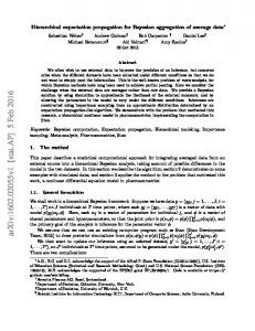
Fig. 2. Area under the ROC Curve (AUC) when ranking papers in the same equivalence class by BOPA’s posterior probability of acceptance. On the left, papers with the same reviewer rating average are considered equivalent. On the right, papers with identical sets of ratings are considered equivalent. Only equivalence classes with more than 10 papers are shown.

that many decisions are not clear-cut and that especially the Meta-Reviewers use their own insights and their interpretation of the review text to make the decisions. The probabilistic nature of the BOPA model makes it possible to verify, if these disagreement rates were expected by the model. In particular, BOPA’s predicted error rate can be computed as X disagreement = min{P (yd = accept|{σ (g); ∀g}), P (yd = reject|{σ (g); ∀g})}. d∈D

(9) For our data, the disagreement as predicted by BOPA is 65.3, which not far off the actual disagreement of 78. This provides a first indication that BOPA is able to quantify the amount of uncertainty in the aggregated reviewer scores. We will further investigate this in Section 3.5. 3.4

Can BOPA distinguish paper quality between papers with the same reviewer scores?

The previous section showed that the amount of disagreement of BOPA does not seem to be better than that of Score Averaging. However, there are biases that may have influenced that statistic. First, the Score Average was readily available in CMT for sorting, which may have biased the Meta-Reviewers’ perception of the paper’s quality. Second, the reviewers acceptance scores are communicated to the authors, but not the BOPA ranks. Thus, going against the cardinal score average requires effort from the Meta-Reviewer to justify that recommendation, which disincentivises the MetaReviewer from deviating from the score average. In order to get results that are unaffected by such biases, we now consider subgroups of papers that have equal bias. First, Figure 2 (left) shows how BOPA performs for

11

Estimated Probability

1 0.8 0.6 0.4 0.2 0 0

0.2

0.4

0.6

0.8

1

Predicted Probability

Fig. 3. Calibration of BOPA posterior acceptance probabilities. Binning is done via quantiles so that each bin contains roughly 40 papers. The x-axis shows the averaged posterior acceptance probabilities, and the y-axis the observed fraction of accepted papers per bin (with 95% binomial confidence intervals).

papers that have the same score average. In particular, for a particular score average value, we rank all papers with that score average by their probability of acceptance P (yd = accept|{σ (g); ∀g}) as predicted by BOPA. The left plot of Figure 2 shows the Area under the ROC Curve (AUC) for all score average values that have at least 10 papers and for which the AUC exists. For most values, the AUC is greater than 0.5, indicating that BOPA sorts the papers better than random. The average AUC over all score averages weighted by the number of papers in the equivalence class is 0.630, which is substantially better than 0.5. The right plot in Figure 2 shows the equivalent results, where the conditioning is not on the score average, but on a particular set of ratings. The weighted AUC here is 0.627. This provides evidence that BOPA is indeed able to mitigate the problem of different reviewer scales, since it is able to identify papers that are more likely to be accepted even if they have exactly the same ratings. However, an alternative explanation is that this may also be affected by bias, since Meta-Reviewers were given the BOPA results, even if late in the decision process. To fully resolve this question beyond doubt, a controlled trial may be necessary.

3.5

How calibrated are the BOPA acceptance probabilities?

The estimated disagreement rate of BOPA already provided some evidence in Section 3.3 that BOPA is able to accurately capture the uncertainty inherent in the review process. We now investigate more closely, if BOPA indeed produces well-calibrated probabilities. In particular, we compute P (yd = accept|{σ (g); ∀g}) as in Equation (8) and ask whether a predicted P (yd = accept|{σ (g); ∀g}) of value p indeed means that the paper d has a p-percent probability of being accepted.

12

Figure 3 shows a calibration plot, where papers are binned by P (yd = accept|{σ (g); ∀g}) falling into specific intervals [p1 , p2 ]. The intervals are selected to include roughly 40 papers each (except the interval closes to 0, which contains 399 papers), and the average value of P (yd = accept|{σ (g); ∀g}) for each bin is plotted on the x-axis. The y-axis shows the ratio of accepted papers in each bin with 95% binomial confidence intervals. For perfectly calibrated prediction probabilities, all points should lie on the diagonal. Overall, calibration of the BOPA probabilities is remarkably good, especially in the high-probability region. This verifies that BOPA does indeed convey an accurate impression of uncertainty, as was desired in our original goals. 3.6

Anecdotal Qualitative Feedback

As mentioned above, the information as illustrated in Figure 1 was emailed to all 68 Meta Reviewer. While we did not ask for a response to this email, 14 Meta Reviewer responded to this email. The vast majority of these responses indicated strong support for providing such information, calling it “helpful” and “useful”. No response raised any concerns or was negative. Several emails included suggestions for how to better present and layout the information, and how to better integrate it with CMT.

4

Conclusions

We investigated how additional information and aggregation of reviewer information can provide decision support to Meta-Reviewers and Program Chairs for making accept/reject decisions. Using data from KDD 2015, we adapted a Bayesian ordinal rank aggregation method to the problem of estimating posterior rank distributions of submissions. Regarding the goal of providing information about uncertainty, we find that the BOPA method indeed captures accurately calibrated probabilites. Regarding the goal of mitigating mismatching reviewer scales, we find evidence that this is also achieved by BOPA. However, final confirmation about whether Meta-Reviewers and Program Chairs actually make better decisions using the additional information can only be conclusively answered through controlled experiments, which are outside the scope of this study.

5

Acknowledgments

This research was funded in part by NSF Awards IIS-1217686, IIS-1247637, IIS-1513692, the JTCII Cornell-Technion Research Fund and a Google PhD Fellowship.

References 1. Arrow, K.J.: Social Choice and Individual Values. Yale University Press, 2nd edn. (Sep 1970), http://cowles.econ.yale.edu/P/cm/m12-2/index.htm 2. Aslam, J.A., Montague, M.: Models for metasearch. In: SIGIR. pp. 276–284 (2001), http: //doi.acm.org/10.1145/383952.384007

13 3. Bradley, R.A., Terry, M.E.: Rank analysis of incomplete block designs: I. the method of paired comparisons. Biometrika 39(3/4), pp. 324–345 (1952), http://www.jstor. org/stable/2334029 4. Chen, X., Bennett, P.N., Collins-Thompson, K., Horvitz, E.: Pairwise ranking aggregation in a crowdsourced setting. In: WSDM. pp. 193–202 (2013), http://doi.acm.org/10. 1145/2433396.2433420 5. Cortes, C., Lawrence, N.: The NIPS experiment (2014), http://inverseprobability.com/2014/12/16/the-nips-experiment/ 6. Dwork, C., Kumar, R., Naor, M., Sivakumar, D.: Rank aggregation methods for the web. In: WWW. pp. 613–622 (2001), http://doi.acm.org/10.1145/371920.372165 7. Kendall, M.: Rank correlation methods. Griffin, London (1948) 8. Liu, T.Y.: Learning to rank for information retrieval. Found. Trends Inf. Retr. 3(3), 225–331 (Mar 2009), http://dx.doi.org/10.1561/1500000016 9. Lu, T., Boutilier, C.: Learning mallows models with pairwise preferences. In: ICML. pp. 145–152 (June 2011) 10. Lu, T., Boutilier, C.E.: The unavailable candidate model: A decision-theoretic view of social choice. In: EC. pp. 263–274 (2010), http://doi.acm.org/10.1145/1807342. 1807385 11. Mallows, C.L.: Non-null ranking models. Biometrika 44(1/2), pp. 114–130 (1957), http: //www.jstor.org/stable/2333244 12. Niu, S., Lan, Y., Guo, J., Cheng, X.: Stochastic rank aggregation. CoRR abs/1309.6852 (2013) 13. Qin, T., Geng, X., Liu, T.Y.: A new probabilistic model for rank aggregation. In: NIPS. pp. 1948–1956 (2010) 14. Raman, K., Joachims, T.: Bayesian ordinal peer grading. In: ACM Conference on Learning at Scale (LS) (2015) 15. Raman, K., Joachims, T.: Methods for ordinal peer grading. In: KDD. pp. 1037–1046. KDD ’14, ACM, New York, NY, USA (2014), http://doi.acm.org/10.1145/ 2623330.2623654 16. Volkovs, M.N., Zemel, R.S.: A flexible generative model for preference aggregation. In: WWW. pp. 479–488 (2012), http://doi.acm.org/10.1145/2187836.2187902