of interest X, given the data D, see e.g. Clyde et al. 1996; Smith ... Our model essentially performs a generalized ridge regression (GRR) (Hoerl and Kennard,.
IMS Collections Contemporary Developments in Bayesian Analysis and Statistical Decision Theory: A Festschrift for William E. Strawderman Vol. 8 (2011) 215–234 c Institute of Mathematical Statistics, 2011 � DOI: 10.1214/11-IMSCOLL815
Bayesian prediction with adaptive ridge estimators David G.T. Denison and Edward I. George AHL and University of Pennsylvania Abstract: The Bayesian linear model framework has become an increasingly popular building block in regression problems. It has been shown to produce models with good predictive power and can be used with basis functions that are nonlinear in the data to provide flexible estimated regression functions. Further, model uncertainty can be accounted for by Bayesian model averaging. We propose a simpler way to account for model uncertainty that is based on generalized ridge regression estimators. This is shown to predict well and to be much more computationally efficient than standard model averaging methods. Further, we demonstrate how to efficiently mix over different sets of basis functions, letting the data determine which are most appropriate for the problem at hand.
Contents 1 Introduction . . . . . . . . . . . . . . 2 The generalized shrinkage model . . 2.1 The canonical regression model 2.2 The model priors . . . . . . . . 2.3 The model likelihood . . . . . . 2.4 Posterior inference . . . . . . . 3 Related models . . . . . . . . . . . . 3.1 Bayesian variable selection . . . 3.2 Ridge and minimax estimators 3.3 Generalized ridge estimators . . 3.4 Setting of the shrinkage prior . 4 Examples . . . . . . . . . . . . . . . 4.1 Simulated example . . . . . . . 4.2 Boston Housing Data . . . . . . 5 Mixing over basis sets . . . . . . . . 6 Discussion . . . . . . . . . . . . . . . Acknowledgments . . . . . . . . . . . . References . . . . . . . . . . . . . . . . .
. . . . . . . . . . . . . . . . . .
. . . . . . . . . . . . . . . . . .
. . . . . . . . . . . . . . . . . .
. . . . . . . . . . . . . . . . . .
. . . . . . . . . . . . . . . . . .
. . . . . . . . . . . . . . . . . .
. . . . . . . . . . . . . . . . . .
. . . . . . . . . . . . . . . . . .
. . . . . . . . . . . . . . . . . .
. . . . . . . . . . . . . . . . . .
. . . . . . . . . . . . . . . . . .
. . . . . . . . . . . . . . . . . .
. . . . . . . . . . . . . . . . . .
. . . . . . . . . . . . . . . . . .
. . . . . . . . . . . . . . . . . .
. . . . . . . . . . . . . . . . . .
. . . . . . . . . . . . . . . . . .
. . . . . . . . . . . . . . . . . .
. . . . . . . . . . . . . . . . . .
. . . . . . . . . . . . . . . . . .
. . . . . . . . . . . . . . . . . .
215 217 217 217 218 218 219 219 220 221 223 224 224 228 229 231 232 233
1. Introduction A key goal of regression modelling using Bayesian model averaging has been to provide good predictions of the response variable at points x within some domain AMS 2000 subject classifications: 62F15, 62J05. Keywords and phrases: Bayesian model averaging, generalized ridge regression, prediction, regression splines, shrinkage. 215
D.G.T. Denison and E.I. George
216
of interest X , given the data D, see e.g. Clyde et al. 1996; Smith and Kohn, 1996; Denison, Mallick and Smith, 1998; Hoeting et al., 1999. The data is typically of the form D = {yi , xi }n1 where yi is the response variable and xi = (xi1 , . . . , xip ) gives the values of the p predictor variables with which the regression is to be performed. Attention is often focused on the linear model (1.1)
Y = Xβ + �,
where Y = (y1 , . . . , yn )� , X = {xij }, β = (β1 , . . . , βp )� is a vector of coefficients and � is a vector of independent normal errors. The model averaging methods are then motivated by assigning positive prior probability to the possibility that only some unknown subset of predictors belong in (1.1), i.e. that only a submodel of (1.1) is needed. More generally, such methods are obtained by putting positive probability on the possibility that the mean of Y lies in some proper subspace of the space spanned by X. The resulting model averaging estimates are a posterior weighted sum of all possible model estimates, and have been recommended as a natural alternative to the strategy of selecting a single high posterior submodel which ignores model uncertainty (Draper 1995). The form of the expected response y at a generic point x = (x1 , . . . , xp ) under such Bayesian model averaging is given by (1.2)
E(y|x, D) =
p � i=1
βi∗ xi , where βi∗ =
�
E(βi |γ, D)p(γ|D),
γ∈M
where γ is the index over the 2p possible models in the complete model space M. Thus predictions made by model selection can be represented simply as a linear combination of all the predictors, x1 , . . . , xp , together with a set of coefficients, β1∗ , . . . , βp∗ . Such coefficients are weighted versions of the least squares estimates � for the full model, and we can write β ∗ = wi β�i for i = 1, . . . , p. In general, (LSE) β i each of these coefficients is shrunk by a different amount so that the wi s are not equal. Further, if each of the possible models has a strictly positive prior probability then wi is non-zero for all i. Consequently all of the predictors are used to make the final prediction of the response, offering the advantage of retaining the influence of all the bases when prediction is the aim, see Copas (1983). This point is also discussed by Lindley (1995), who argues that because the full model contains at least as much information as any submodel, it should naturally be preferred. The attractive predictive properties of shrinkage models is also borne out by the results of Holmes and Denison (1999) who compare shrinkage and selection models in the context of wavelet regression. In this paper, we propose an alternative to model averaging, which places prior uncertainty directly on the shrinkage wi of each of the predictor coefficients. While retaining the advantage of using every predictor in the final predictions, our procedure avoids the computational problems associated with placing prior probability on each of the 2p possible subsets as is done with model averaging. Our model essentially performs a generalized ridge regression (GRR) (Hoerl and Kennard, 1970; Goldstein and Smith, 1974; Hocking et al., 1976) with priors on the shrinkage weights. We find that this model performs well in relation to model averaging approaches, yet the computations involved increase only linearly in p rather than exponentially. The significant decrease in computation time allows us to extend the approach to modelling data with mixtures of basis functions. In this way we can determine which set of basis functions (e.g. cubic regression splines or thin-plate splines) are most supported by the data.
Prediction with ridge estimators
217
In the next Section we give the details of our proposed model with Section 3 describing other related approaches to the problem. Section 4 demonstrates the use of this model both on real datasets in a traditional linear model context, as well as on simulated datasets, highlighting how nonlinear regression can be performed in the linear model framework. In Section 5 we generalize the model to incorporate different basis sets and Section 6 contains a discussion. 2. The generalized shrinkage model 2.1. The canonical regression model Assuming from here on that X is of full rank, we begin by rewriting (1.1) in canonical form. As X � X is positive-definite and symmetric there exists an orthogonal matrix U such that U � X � XU = D, where D is a diagonal matrix of the strictly positive eigenvalues of X � X, i.e. D = diag(λ1 , . . . , λp ). Hence, we find that Y (2.1)
= = =
Xβ + � X(U U � )β + � Zα + �,
where α = U � β and Z = XU . Using this formulation, the LSE of α is given by −1 � � = D−1 Z � Y = diag(λ−1 α 1 , . . . , λp )Z Y . 2.2. The model priors As mentioned in the introduction, our approach is to place priors directly on the amount of shrinkage, wi , where here the posterior mean estimate of αi is given by �i . We do this by considering a normal prior on the coefficients, p(α) = αi∗ = wi α N (0, V ), so that the posterior expectation is given by (2.2)
� α∗ = (D + V −1 )−1 Z � Y = (D + V −1 )−1 Dα,
where V = diag(v1 , . . . , vp ) gives the prior variances of the coefficients. Further, we can write d = tr{(D + V −1 )−1 D} = tr{Z(Z � Z + V −1 )−1 Z � }, where d is a measure of the degrees of freedom of the model (Hastie and Tibshirani, 1990). When d = p (i.e. V −1 = 0) the model relates to the least squares solution to the data and when d = 0 (i.e. V = 0) just a constant function is fit to the data. As the degrees of freedom gives us a good idea about the smoothing properties of the model, it is natural to consider a prior on this rather than on the variances of the coefficients, V . � and equating this with By letting W = diag(w1 , . . . , wp ), writing α∗ = W α (2.2), we find that � � λ 1 v1 λ p vp ,..., W = diag , 1 + λ 1 v1 1 + λ p vp � wi . Hence, using this form for the model so vi = wi /{λi (1−wi )} and d = tr(W ) = we find that wi represents the degrees of freedom associated with the ith canonical predictor. Also, we are naturally led to a specific functional relationship between the prior variances and the degrees of freedom associated with each predictor.
D.G.T. Denison and E.I. George
218
Following the results just shown, we place normal priors on the unknown coefficient values αi , and we choose to define the priors hierarchically using the relationship p(αi , wi ) = p(αi |wi )p(wi ). Further, we assume that the prior over (αi , wi ) is independent of the priors on the other coefficients and weights. This leads to the conditional prior of the coefficients being given by � � � λi (1 − wi ) λi (1 − wi ) 2 (2.3) p(αi |wi ) = exp − αi , 2πwi 2wi for all real αi and i = 1, . . . , p. As wi must lie in the unit interval, a natural prior is the Beta(a, b) distribution, so that (2.4)
p(wi ) =
Γ(a + b) a−1 w (1 − wi )b−1 Γ(a)Γ(b) i
for wi ∈ [0, 1].
The choice of a and b (which must both be strictly positive) allow us to define a wide variety of priors on the shrinkage and their choice will be critical to the performance of the final model. Considerations for setting them are given in Section 3.4. 2.3. The model likelihood We make the standard assumption that the elements of � are independently distributed N (0, σ 2 ) random variables, where σ 2 is the regression variance. Hence the log-likelihood of the data given the model parameters is given by (2.5)
log p(D|α, σ 2 ) = constant −
n 1 log σ 2 − 2 ||Y − Zα||2 . 2 2σ
Further, as p(α|w) is conjugate to this likelihood we can perform the integral � p(D|α, w, σ 2 )p(α|w, σ 2 )dα analytically (e.g. O’Hagan, 1994, Denison et al., 2002) to obtain
p �i2 n 1� wi λi α (2.6) log p(D|w, σ 2 ) = constant − log σ 2 + log(1 − wi ) + 2 2 i=1 σ2 We can see from (2.6) that if σ 2 is known, the log-likelihood can be decomposed into p functions of wi alone. So, if we take the wi to be a priori independent, then the wi are also independent a posteriori, and we can write (2.7)
p(w|D) =
p �
p(wi |D).
i=1
Thus, inference about the wi s can proceed individually and we have reduced the problem of finding a p-dimensional posterior distribution to determining p onedimensional posteriors. A similar approach was outlined in Chipman et al. (1997). 2.4. Posterior inference We now proceed as if the regression variance, σ 2 , is known, to be later replaced by αi for all i to an estimate σ �2 . We see from (1.2) that we need to find αi∗ = E(wi |D)� determine the mean of the predictive distribution on the response. We know that 1 wi p(wi |D)dwi , i = 1, . . . , p, (2.8) E(wi |D) = 0
Prediction with ridge estimators
219
and from Bayes’ Theorem together with (2.4) and (2.6) we find that the posterior density of wi is given by 1
(2.9)
p(wi |D) = � 1 0
wia−1 (1 − wi )b− 2 exp( 12 wi t2i ) 1
wia−1 (1 − wi )b− 2 exp( 12 wi t2i )dwi
,
√ �i /σ. So, from (2.8) and (2.9) we find that the expected shrinkage where ti = λi α performed by our model is of the form �1
(2.10)
E(wi |D) =
1 wia (1 − wi )b− 2 exp( 12 wi t2i )dwi 0 . � 1 a−1 1 wi (1 − wi )b− 2 exp( 12 wi t2i )dwi 0
αi is straightforward and fast. It just involves Hence calculation of the αi∗ = E(wi |D)� the determination of 2p one-dimensional integrals on [0,1]. We may also be interested in the maximum a posteriori (MAP) value of y given x. From (1.2) and (2.7) this is just when each of the wi are set to their posterior modes. The MAP value of wi is readily found by combining (2.4) and (2.6) and partially differentiating this posterior with respect to wi . By setting the resulting expression to zero we find that the turning points of wi are
(t2i + 3 − 2a − 2b) ± (t2i + 3 − 2a − 2b)2 + 8t2i (a − 1) . (2.11) wi = 2t2i By inspection of the second derivative we can find out which of these roots (if any) correspond to a maximum in the posterior and lie between [0,1]. In the next section we shall see how certain choices of a and b lead to interesting models. 3. Related models This section contains descriptions of other Bayesian and non-Bayesian methods for performing coefficient shrinkage. Throughout we show how these models relate to the method we propose, highlighting how good candidates for the prior parameters a and b can be chosen. We begin by describing Bayesian model averaging for linear models and then highlight ridge and generalized ridge estimators. 3.1. Bayesian variable selection A common approach to taking into account model uncertainty in a linear regression context is the Bayesian variable selection methodology originally described in George and McCulloch (1993). This paper suggests assigning an indicator variable γi (∈ {0, 1}) to each predictor and then performing a Gibbs step (Gelfand and Smith, 1990) to sample each γi during each iteration of the sampling algorithm. We can do this simply as, when using standard conjugate priors, we can determine p(γi = 1|D, γ −i ) =
p(D|γ −i , γi = 1) p(D|γ −i , γi = 0) + p(D|γ −i , γi = 1)
analytically, where γ −i refers to all the components of γ except the ith one. This approach has been applied successfully to simple linear regression (Hoeting et al., 1999) as well as nonlinear regression approaches such as spline fitting (Smith
D.G.T. Denison and E.I. George
220
and Kohn, 1996) and wavelets (Clyde et al., 1998). Both Hoeting et al. (1999) and Smith and Kohn (1996) adopt the g-prior specification suggested by Zellner (1986), taking p(β γ , σ 2 ) = N (β|0, cσ 2 (Xγ� Xγ )−1 )Gamma(σ −2 |0, 0), where the γ subscripts denote the design matrix made up of only the columns of X for which γi = 1. In canonical form this reduces to a prior on each coefficient p(αi |σ 2 ) = N (0, (cσ 2 )/λi ). Hence the posterior expectation for each coefficient given the model is γi c α �i , E(αi |γi , D, σ 2 ) = c+1 for all i, and all the coefficients in the model are shrunk by a constant factor. Multiple shrinkage of the coefficients occurs when we take into account model uncertainty. For moderate size p, (e.g. p ≤ 20), modern computation can be exploited to determine p(γ|D) analytically, allowing the exact calculation of � E(y|x, D, γ)p(γ|D). E(y|x, D) = γ∈M
Clyde, DeSimone and Parmigiani (1996) suggested that orthogonalization of the model space is justified when prediction is the aim. They give results demonstrating how their orthogonalization approach can outperform predictions obtained by competing approaches such as stochastic search variable selection of George and McCulloch (1993). We extend their work by placing priors on the degrees of freedom associated with each basis function, wi , rather than assuming that the prior variance of the coefficients is known given the set of indicators γ1 , . . . , γp . 3.2. Ridge and minimax estimators can By setting w1 = · · · = wp = w(∈ [0, 1]), both ridge and minimax estimators � � w I . be motivated from a Bayesian point of view under the prior p(α) = N 0, 1−w Ridge estimators are obtained as posterior means of α for fixed choices of w. Such estimators can perform well in some regions of the parameter space, Dempster et al. (1977), and Volinsky (1997) has demonstrated how ridge estimators may outperform standard Bayesian model averaging for certain prediction tasks. However, ridge estimators can also perform poorly in other regions. Alternatives that avoid such poor performance, are minimax estimators, which uniformly dominate the LSE in terms of weighted or predictive squared error loss (3.1)
PMSE(α) = E||Y� − Y ||2 /σ 2 =
p �
λi E{(� αi − αi )2 }/σ 2 ,
i=1
These can be obtained with a further Bayesian treatment of w. For example, plugging an Bayes estimate of w into the posterior mean of α yields the celebrated James-Stein estimator (James and Stein 1961). Strawderman (1971) obtains a proper Bayes minmax estimator by adopting the prior setup � � w Ip p(α|w) = N 0, and p(w) = (1 − d)(1 − w)−d , 1−w for some d ∈ [0, 1). Using this model Strawderman finds that E(w|D) = 1 −
2 p + 2 − 2d , − �1 1 p−d T T 0 (1 − w) 2 exp( 12 wT )dw
Prediction with ridge estimators
221
√ �p where T = 1 t2i (with ti = λi α �i /σ as above). This estimator is shown to be 1 minimax for p ≥ 5 if d ∈ [ 2 , 1) and for p ≥ 6 for all d ∈ [0, 1). By using particular finite mixture priors on α, George (1986) obtains minimax multiple shrinkage estimators which correspond to model averaging estimators. A key aspect for all of these estimators, is the restriction w1 = · · · = wp = w which allows the estimators to “borrow strength” across predictors. Without this or similar restrictions, the minimax property is lost. 3.3. Generalized ridge estimators Generalized ridge regression (GRR) estimates mimic the model we propose much more closely. These generalize the estimators in the previous subsection by allowing a separate “ridge” parameter for each predictor. A possible setup is to take � � wi (3.2) p(αi |wi ) = N 0, for i = 1, . . . , p, λi (1 − wi ) as in Section 2.2. However, unlike the model we propose, GRR estimators do not express any uncertainty in the wi . Instead, it is chosen to be a deterministic function of the data √ which can be expressed as wi = W (ti ). Here we give, in terms of a α/σ value, functions that correspond to some of the most popular generic t = λ� GRR methods. For further details and motivation see the references given, and for a comparison of their efficacy see Lawless (1981). GRN (e.g. Hoerl and Kennard, 1970): W (t) = (1 + t−2 )−1 . GRI1 (e.g. Hoerl and Kennard, 1970): W (t) = {1 + (1 + t−2 )2 /t2 }−1 . √ 2 GRI (Hemmerle, 1975): W (t) = [{1 − 1 − 4t−2 } t2 ]−1 for t2 > 4 else W (t) = 0. GRP (e.g. Mallows, 1973): W (t) = 1 for t2 > 2 else W (t) = 0. GRC (Mallows, 1973): W (t) = 1 − t−2 for t2 > 1 else W (t) = 0. GRR models gained some popularity about thirty years ago (e.g. Hoerl and Kennard, 1970; Hocking et al., 1976) and were originally motivated because the minimax estimators found gave only modest improvements in MSE over the LSE. One drawback with GRR models is that it is known that they are not minimax (Thisted, 1978), and so cannot dominate the LSE in all situations. We can compare GRR estimators in terms of their predictive mean-squared error (Lawless, 1981) as � − β)||2 = � = ||Y� − Y ||2 = ||X(β PMSE(β)
p �
λi E{(� αi − αi )2 }/σ 2 ,
i=1
which, assuming normality and taking σ as known (or fixed), we find that p ∞ � � = (3.3) PMSE(β) {W (zi )zi − μi }2 dFμi (zi ), i=1
−∞
where each zi ∼ N (μi , 1) = Fμi . These one-dimensional integrals, although not analytically tractable, can easily be solved by standard numerical analysis techniques. In Fig. 1 we display (as in Fig. 1 Lawless (1981)) the PMSEs for the five given GRR methods (for p = 1) over the range of values of μ on which they differ significantly. Note that the PMSE associated with the LSE is one for all values of μ. Also, we see that GRN appears the most stable GRR estimator over a wide range of values, significantly reducing the PMSE at low values of μ and only having noticeably worse performance than the LSE for 2 < μ < 6.
D.G.T. Denison and E.I. George
222 3
2.5
Theoretical MSE
2
1.5
1
0.5
0
0
1
2
3
4
5 mu
6
7
8
9
10
Fig 1. Theoretical PMSE curves for the GRR estimators of Section 3.3. Here the curve for GRN has the lowest mode.
In general, we see that GRR estimators perform best when the dataset corresponds to many low values of μ(< 1.5) as well as high values μ > 8. This is because great gains in terms of PMSE are possible at the low values of μ and negligible losses occur at high values. This falls in line with general thinking which suggests that GRR estimates are particularly effective when X � X is ill-conditioned. We can compare the performance of GRR models and an orthogonalized Bayesian model for which we estimate σ 2 and take the g-prior specification for the coefficients, so that p(α) = (0, cD−1 ). Consider the posterior expectation of the ith coefficient we see that E(αi |D) =
p(γi = 1|D)E(αi |γi , D) c h(μi ) × α �i , = 1 + h(μi ) 1 + c
where
(c + 1)− 2 exp{0.5cμ2 /(1 + c)} 1
h(μ) =
(c + 1)− 2 exp{0.5cμ2 /(1 + c)} + 1 1
.
From this expression, we can analytically determine the shrinkage performed by the Bayesian model for any value of μ. This is given by W (μ) =
c h(μ) , 1 + h(μ) 1 + c
and this function can be directly compared with those for the other GRR estimators. In Fig. 2 we plot the PMSEs for the orthogonalized Bayesian model for various values of c. Note that the default choice for c is often the size of the dataset n. We see that as c increases the PMSE properties become increasingly poor for 1.5 < μ < 5.5. However, improvements are found for μ < 1 for larger values of c. Fig. 2 suggests that we need to determine Bayesian models with much better PMSE properties than the orthogonalized model in order to predict consistently well.
Prediction with ridge estimators
223
3
2.5
Theoretical MSE
2
1.5
1
0.5
0
0
1
2
3
4
5 mu
6
7
8
9
10
Fig 2. Theoretical PMSE curves for the orthogonalized Bayesian model for various values of c (as well as the GRN curve for reference with Fig. 1): GRN (thick solid line); c = 50 (dashed); c = 200 (dotted); c = 500 (dot-dashed) and c = 1000 (thin solid).
3.4. Setting of the shrinkage prior This subsection highlights how certain GRR models are special cases of Bayes estimators using the proposed models. These relate to certain choices of a and b in the Beta(a, b) prior on the wi , and making inference with the posterior mode. We include this subsection only to demonstrate some features of the model as we do not suggest using the posterior mode to minimise predictive squared error. This would only be chosen under a 0-1 loss function. Note that we let w �i denote any posterior mode of wi that lies in the unit interval. 1. a = 1, b > 0: w �i = max{1 − (2b − 1)μ−2 i , 0}. So for the special case when b = 1 we perform exactly the same shrinkage as GRC when using the MAP value of wi to make inference. Also, this specification corresponds to choosing a uniform prior on the shrinkage. Further, for b > 1 the amount of shrinkage of α �i is always greater than GRC and for 0 < b < 1 the shrinkage is always less than GRC. Also note that for 0 < b ≤ 12 the MAP estimate is degenerate and corresponds to taking w �i = 1 for all i (i.e. we choose to fit with the least squares estimates in every dimension). It is also worth pointing out that for 0 < b ≤ 1 we are assigning a Strawderman prior on wi with d = 1−b, although he advocates always using the expected shrinkage to make inference. 2. a = b > 0: This setting is attractive as it ensures that the prior on wi is symmetric and E(wi ) = 12 . The amount of prior mass located around 0 and 1 depends on the magnitude of b(= a). We feel that values of b less than 1 are most appropriate as they relate to priors which have more prior mass at the extremities than at 12 . Thus the LSE are more likely to be shrunk either a small amount or a large amount and unlikely to be shrunk by values near 1 take b = 0.75. 2 . Here we just highlight the special case we obtain when we Here we find that the MAP shrinkage function is w �i = 0.5 + μ2i − 2/(2μi ) 2 for μi > 2 and zero otherwise. Note that this shrinkage function is most
D.G.T. Denison and E.I. George
224 3
2.5
Theoretical MSE
2
1.5
1
0.5
0
0
1
2
3
4
5 mu
6
7
8
9
10
Fig 3. Theoretical PMSE curves for some Bayesian mean GRR estimators with various settings of a and b (as well as the GRN curve for reference with Fig. 1): GRN (thick solid line); a = b = 1 (dashed); a = 1, b → 0 (dot-dashed); a = b = 0.75 (dotted) and a = 2, b → 0 (thin solid).
closely related to GRP except that it does not suggest such a strong “shrinkor-select” approach. The threshold for having non-zero coefficients is identical but shrinkage is still performed on those retained in the model. Undoubtedly other interesting settings are available that relate to previous work but these two classes are given as examples of how the methodology relates to other GRR approaches. In Fig. 3 we display the PMSE curves for various settings of a and b taking our estimate to the shrinkage to be the posterior expectation. We find that for settings a = 1 and a = 2 together with b → 0 (which in practice we took as b = 0.001) we obtain estimators that are more stable than GRN in the sense that they are more conservative at low values of μ but have less errors at middling values. In fact as a increases and b stays around zero we get progressively flatter PMSE curves as less shrinkage is performed at all values of μ. Also, we see that in some cases, for instance a = b = 1, inference using the posterior mean can lead to quite unstable shrinkage estimators when compared with the MAP estimator (GRC in Fig. 1). In these cases (a = b = 1 and a = b = 0.75) the most significant source of error is when the posterior mean estimate shrinkage is too great for large values of μ. In comparison, for these values the MAP estimate performs no shrinkage at all. 4. Examples 4.1. Simulated example This simulation study is not intended to be exhaustive but illustrative. We shall try and show why the model we propose predicts better than the standard Bayesian model averaging approach using model selection. We shall use a simple curve-fitting example. Although this involves the estimation of the response with respect to a single predictor variable when using flexible (nonlinear) basis functions that depend
Prediction with ridge estimators
225
���
�
���
�
���
�
����
�
���
���
���
���
���
���
��
��
���
�
Fig 4. A realization of the first simulated dataset with σ = 0.3 together with the truth (solid line).
on the predictor value this is identical to a multiple regression problem. Hence we observe data D = (yi , xi )ni=1 and we assume the relationship yi =
p �
βj Bj (xi ) + �i ,
j=1
where �i ∼ N (0, σ 2 ) and the {B1 , . . . , Bp } are a set of basis functions that are fixed before the analysis. Smith and Kohn (1996) suggest using the cubic regression spline basis. In this example we shall use a spline basis but choose fewer basis functions than they suggest so that we can perform the analysis exactly rather than approximately via simulation. This ensures that the comparison between methodologies is more transparent and does not depend on how various parameters that control the simulation algorithm are set. Hence, for this example we took Bj (x) = xj , j = 1, 2, 3 and Bj (x) = [x − (j − 3)/(p − 2)]3+ , j = 4, . . . , p, where [a]+ = max(a, 0) and the size of the complete model space only involves 2p models. The prior we assign over the coefficients is β ∼ N (0, nσ 2 (X � X)−1 ) as suggested in Kohn, Smith and Chan (2000) and Gustafson (2000). For this example we use a similar test function to that given in Fan and Gijbels (1996) and take yi = 2xi + exp{−64(2xi − 1)2 } + �i ;
i = 1, . . . , n,
where the xi ∼ U [0, 1], �i ∼ N (0, σ ) and n = 200. An example of such a dataset is given in Fig. 4. To approximate the error of the reconstructions to the true function we calculate the sum of squared errors (SSE) given by as 2
SSE =
200 � i=0
{f (i/200) − f�(i/200)}2 ,
D.G.T. Denison and E.I. George
226
Table 1 Results in terms of SSE over 100 randomly generated datasets for the simulated example with n = 200 and using the cubic regression spline basis with various values of σ and p. Standard errors of the estimates are superscripted. For each setting the result with the lowest ISE is given in italics. p 8 8 10 10 12 12 14 14
σ 0.2 0.3 0.2 0.3 0.2 0.3 0.2 0.3
BMA 2.6940.018 3.2830.053 1.3460.024 1.8030.037 0.7070.027 1.2200.050 0.4350.019 1.0640.049
GRN 2.5400.016 3.0220.046 1.2720.022 1.6710.038 0.7320.031 1.2950.048 0.6110.025 1.3520.063
BGR1 2.5430.016 3.0150.046 1.2650.022 1.6700.038 0.7210.031 1.3170.050 0.6230.026 1.3670.062
BGR2 2.5470.016 3.0160.045 1.2680.022 1.6870.038 0.7290.032 1.3540.051 0.6420.026 1.4150.064
STR 2.5600.017 3.0370.042 1.2960.023 1.7640.041 0.7660.033 1.4520.055 0.6960.027 1.5540.073
LSE 2.5600.017 3.0450.043 1.2990.023 1.7650.041 0.7670.033 1.4650.055 0.6990.027 1.5650.073
where f�(x) is the mean of the predictive density of y at x. Remember that the posterior mean prediction should minimise squared-error loss. In Table 1 we display the results taking n = 200 and differing values of σ(0.2 and 0.3), and differing number of basis functions (p = 8, 10, 12, 14). In this table BMA stands for the Bayesian posterior weighted selection model of Section 3.1, GRN the method given in Section 3.3, BGR1 and BGR2 the method proposed taking b = 0.001 with a = 1 and a = 2 respectively, STR the Strawderman method of Section 3.2 with a = 0.5 so that it is minimax for p ≥ 5 (Strawderman, 1971) and LSE is just the standard least-squares method with no shrinkage. In all the simulations σ is set to its true value with 0.2 corresponding to a low noise setting (signal-to-noise ratio (SNR) of 10) and 0.3 corresponding to a high noise setting (SNR of 4). We see from Table 1 that the BMA performs poorly in terms of prediction across the simulations, sometimes even worse than the simple LSE. The best two models are GRN and BGR2 and from Fig. 3 we can see why these should perform similarly. We know that the basis functions for these types of splines are highly correlated leading to an ill-conditioned X � X matrix. This is why generalized ridge shrinkage seems to be performing well, especially for those shrinkage methods that perform well over small values of μ. Further, with the high noise setting we see a degradation of performance of the methods from p = 12 to p = 14, most probably due to numerical instabilities. This suggests that we cannot add more potential knot sites with impunity and this setting is important in obtaining good results. In Table 2 we repeat the experiment of Table 1 using models with the same number of knot points but with thin-plate spline basis functions, rather than the cubic ones. These take the form B1 (x) = x, and Bj (x) = {x − (j − 1)/p}2 log |x − (j − 1)/p|, j = 2, . . . , p, and lead to better conditioned X � X matrices. From Table 2 we can also see that these basis functions approximate the true curve better for the same value of p. Now, because of the better conditioning of X � X the best model appears to be BGR1 which performs better over a wide range of values of μ. Also, the models that perform the least shrinkage (STR and LSE) also perform well. This is to be expected as we are less likely to have as many small eigenvalues of X � X now. However, the better conditioned matrix has not helped BMA as it actually performs worse than least-squares estimate for every setting of p and σ. In Fig. 5 we plot the SSE for the BMA method with various settings of c. Smith and Kohn (1996) and Gustafson (2000) both suggest taking c = n(= 200) and we
Prediction with ridge estimators
227
Table 2 Same as Table 1 but using the thin-plate spline basis. p 6 6 8 8 10 10 12 12
σ 0.2 0.3 0.2 0.3 0.2 0.3 0.2 0.3
BMA 2.7040.028 3.0250.037 1.1120.026 1.5520.048 0.5360.020 0.8820.036 0.3710.018 0.7490.034
GRN 2.6180.024 2.9070.035 1.0760.021 1.4120.041 0.5710.018 1.0440.041 0.5270.018 1.1200.053
BGR1 2.6100.024 2.8840.034 1.0660.021 1.3970.041 0.5690.018 1.0320.041 0.5280.019 1.1040.049
BGR2 2.6010.023 2.8760.034 1.0610.021 1.3940.041 0.5680.018 1.0280.040 0.5240.018 1.0950.048
STR 2.5950.023 2.8810.035 1.0630.020 1.4160.042 0.5740.018 1.0550.042 0.5270.018 1.1370.047
LSE 2.5950.023 2.8840.035 1.0630.020 1.4210.042 0.5740.018 1.0610.043 0.5280.018 1.1460.048
Fig 5. The average SSE from 100 randomly generated dataset for the simulated example with 7 knots at 0.125 to 0.875, inclusive. The diamonds on the solid line are the average SSE for the BMA model using thin-plate splines with c given on the horizontal axis. The squares on the dashed line are the same but for the cubic spline model. The horizontal lines are the results for the BGR1 model (solid – thin-plate, dashed – cubic).
see that this is one of the better values for these two datasets. However, whatever value of c is chosen, neither of these models ever beat, in terms of SSE, the BGR1 method displayed or the BGR2 one which is not shown. This suggests a weakness of the BMA framework which we now try and explain. The difference in performance of the methods is mainly due to the conditioning of the X � X matrix and how the methods cope with the values of μ in different ranges. We find that the eigenvalues and μ values for a typical dataset using cubic splines with p = 10 are given by λ: μ:
3.48 × 10⁻⁷ , 4.39 × 10⁻⁷ , 1.94 × 10⁻⁶ , 7.10 × 10⁻⁶ , 3.17 × 10⁻⁵ 0.000270, 0.00317, 0.111, 5.96, 145 3.85, 0.499, 6.41, −1.46, 6.70, 0.174, 5.81, 2.07, −16.4, 57.4.
We immediately see that the condition number for the matrix is large (4.17 × 108 = |λ10 |/|λ1 |). This suggests that ridge techniques should perform well as they automatically condition the matrix that needs to be inverted to obtain the coefficient
D.G.T. Denison and E.I. George
228
estimates, in contrast to the LSE and the BMA method described here. Also, as only two of the μ are low we cannot improve greatly over LSE but modest improvements are possible. Remember that examples for which there are many small μ values will be particularly well suited to the methods we suggest. In contrast, for the thin-plate spline model we find λ: μ:
0.000238, 0.000292, 0.00127, 0.00144, 0.0157, 0.0174, 0.359, 2.08, 6.07, 83.0 101, 12.9, 164, −20.9, 149, 1.40, 61.7, 8.95, −16.5, 43.5.
As well as the condition number being far smaller for this basis set we see that the μ values are in general high. As GRR estimators and the LSE are almost identical for μ > 10 both approaches give similar results (Table 2). This demonstrates how the efficacy of the methods, measured via the PMSE, are dependent on product of the square-rooted eigenvalues and the least-squares estimates, not just on the absolute values of the eigenvalues as is sometimes assumed. 4.2. Boston Housing Data The Boston Housing Data of Harrison and Rubenfeld (1978) is a well-known benchmark test dataset. The regression problem involves predicting the median price of owner occupied homes in Boston on the basis of 13 predictor variables listed in Table 4.1 of Denison et al. (2002). The overall model we chose to fit was a standard linear one where each predictor variable had an associated slope coefficient. The dataset contains 506 datapoints in total but, following Quinlan (1993), to test the predictive power of the various methods we adopt a ten-fold cross-validation approach. Hence, in each case we fitted a linear model to each training dataset and then determined the SSE over the corresponding test sets. From Table 3 we see that the ridge methods perform acceptably, but only on a par with the LSE, which predicts well, probably due to the better conditioning of the X � X matrix in this “typical” linear regression problem. However, BMA again fails to demonstrate significant advantages over the other, much simpler, methods when we are looking to make predictions. Nevertheless, BMA would provide us with information about subsets of the 13 predictors that predict acceptably: information that is not so easy to come by with the other ridge methods. Note that the results for the BMA approach took around 2587 million floating point operation whereas much less than a million were required for BGR1 and BGR2. Table 3 Results in terms of SSE for the Boston housing dataset using 10 splits of the data into training and test sets. CV Set 1 2 3 4 5 6 7 8 9 10 Mean
BMA 20.42 22.61 25.63 30.47 19.25 30.39 30.89 18.70 16.40 13.57 22.83
GRN 20.70 21.42 25.01 30.96 18.98 30.65 31.18 18.04 15.67 13.55 22.62
BGR1 20.61 21.48 25.10 30.91 19.02 30.60 31.11 18.10 15.45 13.60 22.60
BGR2 20.45 21.64 25.18 30.85 19.04 30.53 31.00 17.99 15.41 13.63 22.57
STR 20.16 22.27 25.37 30.77 19.05 30.36 30.76 17.80 15.44 13.81 22.58
LSE 20.12 22.12 25.48 30.75 19.04 30.38 30.79 17.74 15.59 13.78 22.58
Prediction with ridge estimators
229
5. Mixing over basis sets As we can see from the results in Tables 1 and 2, the two sets of basis functions give different results in terms of SSE for similar numbers of knots. In fact, it is known that no one method will dominate all others for every problem so the basis set to use is certainly important. We also see the strong dependence between the number of candidate knot sites and the prediction errors. So, in order to provide good predictions this too should be chosen with care. We should not just put down far more knots than we need as this has implications in terms of the condition number of the design matrix. Fortunately, as the method we employ for shrinkage estimation is so quick we can allow the method to determine the number of candidate knot sites to use and, potentially as important, the basis set to use. In the past both of these choices have been, to at least some extent, left to chance and not well discussed. To tie in with the earlier work in this paper we shall restrict ourselves to outlining the approach with the two basis sets described earlier: the cubic regression spline and the thin-plate spline. Further, we allow the number of candidate knot sites to vary from 4 to 30 knots, evenly spaced along [0,1]. We shall consider a second test function and simulated 200 points from the model yi = sin(6xi ) + 2 exp(−64(2x − 1)2 ) + �i , where the �i are independently distributed N (0, 0.32 ) random variables, xi ∼ U [0, 1]. An example of such a dataset is given in Fig. 6. Let K denote the number of candidate knot sites and MT and MC denote the thin-plate and cubic regression spline models. In this way we have introduced extra randomness into our model and now we wish to make inference about p(w, K, M|D), rather than just the posterior distribution of the weights. To compare the relative merits of the different basis sets and numbers of candidate knot locations we can determine the model with the largest marginal likelihood �
���
�
���
�
���
�
����
��
����
��
�
���
���
���
���
���
���
��
��
���
�
Fig 6. A realisation of the second simulated dataset (σ = 0.3) together with the truth (solid line).
D.G.T. Denison and E.I. George
230 970
960
Log marginal likelihood
950
940
930
920
910
5
10
15 20 Number of knots
25
30
Fig 7. The log marginal likelihood for the thin-plate (circles) and cubic (squares) spline models with varying numbers of candidate knot locations.
given K and the model M. This is just the product of the denominators in (11). Recall that this is simple to compute as it just involves a product of univariate integrals. Note that picking the model with the largest marginal likelihood (ML), conditioned on K and M, is equivalent to picking the maximum a posteriori model under uniform priors on K and the basis set to use. The simplest way to calculate the ML is using Monte Carlo integration. We can do this by first determining the eigenvalues and least squares estimates relating to √ a model with a specified K and basis set. This allows us to calculate the μi = λi α �i /� σ (i = 1, . . . , p) for that model. Then, by generating J (a large value we typically take as 10,000) Beta(a, b + 0.5) random variables W 1 , . . . , W J , we find that the log ML, up to an additive constant, is given by ⎧ ⎫⎤ ⎡
p J ⎨ ⎬ � � Γ(a)Γ(b + 12 ) 1 1 j 2 ⎦. ⎣μ2i + 2 log + (W exp[ − 1)μ ] p log i ⎩ ⎭ 2 2 Γ(a + b + 12 ) i=1
j=1
Using this form avoids overflows in the exponential term. To perform the analysis we used the BGR1 prior (a = 1, b = 0.001) and took σ � to be the median absolute deviation of the residuals given the thin-plate spline model with 30 knots. Note that the results shown took only one minute of computing time to produce using MATLAB. In Fig. 7 we display the log marginal likelihood for both the thin-plate spline and the cubic spline models for each value of K. We see that the model with the largest ML is the one that uses the thin-plate spline basis set with 11 candidate knots. Note this only means that the shrinkage is performed with these 11 thinplate spline bases and that not all of these basis functions will have a significant coefficient. With 11 bases it seems that a balance has been reached between the flexibility of the model and the poor conditioning of the X � X matrix.
Prediction with ridge estimators
231
10
9
8
7
SSE
6
5
4
3
2
1
0
5
10
15 20 Number of knots
25
30
Fig 8. The same as for Fig. 7 but for the sum of squared errors (SSE).
Fig. 8 gives the SSE for each of the models under consideration. We see that the one with the largest ML is indeed the one with the lowest prediction error rate (SSE=1.123 with K = 11 and under MT ). From experience with the model, we note that this appears to often be the case. We know that Bayesian prediction should be done with reference to the posterior predictive distribution p(y|x, D) with all the random parameters integrated. This is straightforward in this context as it just involves further summations of the marginal likelihood determined earlier over the possible values of K and the two models under consideration. Unsurprisingly, using the fully marginalised posterior predictive reduces the SSE even further to 1.097 from 1.123 for the best error rate using any single model looked at. This mean estimate produced in this way is plotted in Fig. 9. This sort of increased predictive performance is typically found when averaging over models. Even though these results were found using only one simulation they are typical of what we would expect to see. We have already demonstrated the efficacy of the model for prediction so this section is included mainly to show how, by using such an efficient model averaging scheme, we can average over possible candidate basis sets. Further, we can even take into account the misspecification associated with using a single set of candidate knot sites which can be significant and cannot be chosen arbitrarily large. 6. Discussion We have proposed a new method for performing generalized shrinkage which assumes that the prior on the coefficients is a Beta mixture of normal distributions. This method proposed is computationally efficient and has been shown to outperform standard BMA models for spline fitting, a context for which they have recently gained a lot of popularity (e.g. Smith and Kohn, 1996; Denison, Mallick and Smith, 1998; Gustafson, 2000).
D.G.T. Denison and E.I. George
232 ���
�
���
�
���
�
����
��
����
�
���
���
���
���
���
���
��
��
���
�
Fig 9. The expectation of the mean of the posterior predictive distribution (dashed line) found by averaging over both the number of candidate knots and the two basis sets. The true curve is given by the solid line.
Standard Bayesian model averaging does not always perform so poorly as the results in this paper suggest. We have come across examples when it outperforms the simple GRR methods when the μi for the datasets are of similar size and roughly between 1 and 10. These are the situations where GRR methods are at their worst (see Figs. 1 and 3). Nevertheless we have shown that we cannot blindly put our faith in model averaging. Its performance is dependent on the dataset we wish to analyse. This paper is not intended to criticise Bayesian model averaging per se. It only demonstrates weaknesses in the usual model averaging framework employed (Section 3.1). The Bayesian GRR methods we adopt also incorporates model uncertainty as we also make inference using the posterior expectation of the unknown parameters. Also, both methods perform multiple shrinkage of the coefficients. However, we feel that in our framework the unknowns are more interpretable and lead to priors on the coefficients which turn out to be scaled Beta mixtures of normal distributions rather than the conjugate normal density. Such mixture densities have been shown to be particularly effective for prediction (e.g. Clyde and George, 2000). Acknowledgments This work was carried out while the first author was visiting the second author at University of Texas at Austin. The first author was funded by an EPSRC Overseas Travel Grant, was supported by the Nuffield Foundation and acknowledges the helpful comments provided by Chris Holmes. The second author was funded by NSF grants DMS-98.03756, DMS0130819, DMS-0605102 and Texas ARP grant 003658.690. The authors are grateful to Eric Marchand for helpful suggestions. This article is based on an unpublished 2000 technical report by the same name.
Prediction with ridge estimators
233
References Chipman, H., Kolaczyk, E.D. and McCulloch, R.E. (1997) Adaptive Bayesian wavelet shrinkage. J. Am. Statist. Assoc., 92, 1413–1421. Clyde, M., DeSimone, H. and Parmigiani, G. (1996) Prediction via orthogonalized model mixing. J. Am. Statist. Assoc., 91, 1197–1208. Clyde, M., Parmigiani, G. and Vidakovic, B. (1998) Multiple shrinkage and subset selection in wavelets. J. Am. Statist. Assoc., 92, 391–402. Clyde, M. and George, E.I. (2000) Flexible empirical Bayes estimation for wavelets. J. Roy. Statist. Soc. B, 62, 681–698. Copas, J.B. (1983) Regression, prediction and shrinkage (with discussion), J. Roy. Statist. Soc. B, 45, 311–354. Dempster, A.P., Schatzoff, M. and Wermuth, N. (1977) A simulation study of alternatives to ordinary least squares. J. Am. Statist. Assoc., 72, 77–106. Denison, D.G.T., Mallick, B.K. and Smith, A.F.M. (1998) Automatic Bayesian curve fitting. J. Roy. Statist. Soc. B, 60, 333–350. Denison, D.G.T., Holmes, C.C., Mallick, B.K. and Smith, A.F.M. (2002) Bayesian Methods for Nonlinear Classification and Regression. Chichester: Wiley. Draper, D. (1995) Assessment and propogation of model uncertainty (with discussion). J. Roy. Statist. Soc. B, 57, 45–97. Fan, J.Q. and Gijbels, I. (1995) Data-driven bandwidth selection in local polynomial fitting – Variable bandwidth and spatial adaption. J. Roy. Statist. Soc., 57, 371–394. Gelfand, A.E. and Smith, A.F.M. (1990) Sampling based approaches to calculating marginal densities. J. Am. Statist. Assoc., 85, 398–409. George, E.I. (1986). Minimax multiple shrinkage estimation. Ann. Statist., 14, 188–205. George, E.I. and McCulloch, R.E. (1993) Variable selection via Gibbs sampling. J. Am. Statist. Assoc., 88, 881–889. Goldstein, M. and Smith, A.F.M. (1974) Ridge-type estimators for regression analysis. J. Roy. Statist. Soc. B, 36, 284–291. Gustafson, P. (2000) Bayesian regression modeling with interactions and smooth effects. J. Am. Statist. Assoc., 95, 795–806. Harrison, D. and Rubenfeld, D.L. (1978) Hedonic housing prices and the demand for clean air. J. Environ. Econ. Manag., 5, 81–102. Hastie, T.J. and Tibshirani, R.J. (1990) Generalized Additive Models. London: Chapman & Hall. Hemmerle, W.J. (1975) An explicit solution for generalized ridge regression. Technometrics, 17, 309–314. Hocking, R.R., Speed, F.M. and Lynn, M.J. (1976) A class of biased estimators in linear regression. Technometrics, 18, 425–437. Hoerl, A.E. and Kennard, R.W. (1970) Ridge regression: biased estimation for nonorthogonal problems. Technometrics, 12, 55–67. Hoeting, J.A., Madigan, D., Raftery, A.E. and Volinsky, C.T. (1999) Bayesian model averaging: A tutorial (with discussion). Statist. Sci., 14, 382– 417. Holmes, C.C. and Denison, D.G.T. (1999) Bayesian wavelet analysis with a model complexity prior. In Bayesian statistics 6 (Eds. J.M. Bernardo, J.O. Berger, A.P. Dawid and A.F.M. Smith), pp. 769–776. Oxford: Clarendon Press. James, W. and Stein, C.M. (1961) Estimation with quadratic loss. Proc. 4th Berkeley Symposium 1, 361–379.
234
D.G.T. Denison and E.I. George
Kohn, R., Smith, M. and Chan, D. (2000) Nonparametric regression using linear combinations of basis functions. Technical report., Australian Graduate School of Management, University of New South Wales. Lawless, J.F. (1981) Mean squared error properties of generalized ridge estimators. J. Am. Statist. Assoc., 76, 462–466. Lindley, D.V. (1995) Discussion of “Assessment and propogation of uncertainty” by D. Draper. J. Roy. Statist. Soc. B, 57, 75. Mallows, C.L. (1973) Some comments on Cp . Technometrics, 15, 661–675. O’Hagan, A. (1994) Kendall’s Advanced theory of statistics: Bayesian Inference. Cambridge: Arnold. Quinlan, R. (1993) Combining instance-based and model-based learning. Machine Learning: Proc. 10th Int. Conf., Amherst, MA, 1993. Morgan Kaufmann. Smith, M. and Kohn, R. (1996) Nonparametric regression using Bayesian variable selection. J. Econometrics, 75, 317–344. Strawderman, W.E. (1971) Proper Bayes minimax estimators of the multivariate normal mean. Ann. Math. Statist., 42, 385–388. Thisted, R.A. (1978) On generalized ridge regression. Technical report No. 57, Dept. of Statistics, University of Chicago. Volinsky, C.T. (1997) Bayesian model averaging for censored survival data. PhD Thesis, University of Washington, Seattle. Zellner, A. (1986) On assessing prior distributions and Bayesian regression analysis with g-prior distributions. In Bayesian inference and decision techniques: Essays in honor of Bruno de Finetti (Eds. P.K. Goel and A. Zellner). Amsterdam: North Holland.