In order to address these challenges a robot capable of autonomously exploring densely populated urban environments is created within the Autonomous City.
Bayesian State Estimation and Behavior Selection for Autonomous Robotic Exploration in Dynamic Environments Georgios Lidoris, Dirk Wollherr and Martin Buss Abstract— In order to be truly autonomous, robots that operate in natural, populated environments must have the ability to create a model of these unpredictable dynamic environments and make use of this self-acquired uncertain knowledge to decide about their actions. A formal Bayesian framework is introduced, which enables recursive estimation of a dynamic environment model and action selection based on this estimate. Existing methods are combined to produce a working implementation of the proposed framework. A RaoBlackwellized particle filter (RBPF) is deployed to address the Simultaneous Localization And Mapping (SLAM) problem and combined with recursive conditional particle filters in order to track people in the vicinity of the robot. In this way, a complete model is provided, which is utilized for selecting the actions of the robot so that its uncertainty is kept under control and the likelihood of achieving its goals is increased. All developed algorithms have been applied to the domain of the Autonomous City Explorer robot and results from the implementation on the robotic platform are presented.
I. INTRODUCTION A long term goal of robotics is to bring robots into the real world, enable them to operate efficiently and safely in natural, populated environments, and become part of our everyday lives. This requires robots with complex cognitive capabilities that can achieve higher levels of cooperation and interaction with humans. In order to address these challenges a robot capable of autonomously exploring densely populated urban environments is created within the Autonomous City Explorer (ACE) project [1]. To be truly autonomous such a system must be able to create a model of its unpredictable dynamic environment, based on noisy sensor information and reason about it. More specifically, a robot is envisioned that is able to find its way in an urban area, without a city map or GPS. In order to find its target the robot will approach pedestrians and ask for directions. Due to sensor limitations the robot can observe only a small part of its environment and these observations are corrupted by noise. By integrating successive observations a map can be created, but since also the motion of the robot is subject to error, the mapping problem comprises also a localization problem. This duality constitutes the Simultaneous Localization And Mapping (SLAM) problem. In dynamic environments the problem becomes more challenging since the presence of moving obstacles can complicate data association and lead to incorrect maps. Moving entities must be identified and their future position needs to be predicted over a finite time horizon. The autonomous sensory-motor system G. Lidoris, D. Wollherr and M. Buss are with the Institute of Automatic Control Engineering (LSR), Technische Universit¨at M¨unchen, D-80290 M¨unchen, Germany, {georgios.lidoris, dw, mb}@tum.de
is finally called to make use of its self-acquired uncertain knowledge to decide about its actions. The problem of SLAM is one of the fundamental problems in robotics and has been studied extensively over the last years. The most popular approach [2] is based on the Extended Kalman Filter (EKF). This approach is relatively effective since the resulting estimated posterior is fully correlated about landmark maps and robot poses. Its disadvantage is that motion model and sensor noise are assumed Gaussian and it does not scale well to large maps, since the full correlation matrix is maintained. To overcome these drawbacks particle filters have been used as an effective means for state estimation. This framework has been extended, in order to approach the SLAM problem with landmark maps in [3]. In [4] a technique is introduced to improve grid-based Rao-Blackwellized SLAM. A similar approach is taken here with the difference that scan-matching is not performed in a per-particle basis but only before new odometric measurements are used by the filter. This way better performance is achieved. Until now, no complete Bayesian framework exists for the dynamic environment mapping problem. One of the first attempts was introduced in [5]. In [6] scan registration techniques are used to match raw measurement data to estimated occupancy grids in order to solve the data association problem and the Expectation-Maximization algorithm is used to create a map of the environment. A drawback is that the number of dynamic objects must be known in advance. Particle filters have been used to track the state of moving objects in [7]. However the static environment is assumed known. Particle filters have also been used in [8] to solve the data association problem for mapping but without considering robot localization. In robotics, action selection is related to optimization. Actions are selected so that the utility toward the goal of the robot is maximized. Reviews on action selection in robotics have been presented in [9], [10]. The first contribution of this paper is the introduction of a formal Bayesian framework that enables recursive estimation of a dynamic environment model and action selection based on these uncertain estimates. This is presented in Section II. In Section III, it is shown how existing methods can be combined to produce a working implementation of the proposed framework. A Rao-Blackwellized particle filter (RBPF) is deployed to address the SLAM problem and combined with recursive conditional particle filters in order to track people in the vicinity of the robot. Conditional filters have been used in the literature for tracking given an a
Fig. 1. The Autonomous City Explorer (ACE) robotic platform, which was used for the experiments.
priori known map. In this paper they are modified to be utilized with incrementally constructed maps. This way a complete model of dynamic, populated environments can be provided. Estimations serve as the basis for all decisions and actions of robots acting in the real world. In Section IV these estimations are combined with concepts from information theory and the field of robotic exploration and criteria are formulated to characterize the effect of future actions. These are utilized for coordinating the behaviors of the robot so that uncertainty is kept under control and the likelihood of achieving its goals is increased. Finally, results from the implementation of the proposed algorithms on the ACE robotic platform, that is depicted in Fig. 1, are presented in Section V. II. BAYESIAN FRAMEWORK A Bayesian approach is taken in this paper in order to deal with uncertain system state knowledge and uncertain sensory information, while selecting the behaviors of the system. The main inspiration behind this approach is derived from the human cognition mechanisms. According to [11], action selection is a fundamental decision process for humans, and depends on the state of both body and the environment. Signals in the human sensory and motor systems are corrupted by variability or noise. Therefore the nervous system needs to estimate these states. Recent studies that have investigated the mechanisms used by the human nervous system to solve such estimation and decision problems, have shown that human behavior is close to that predicted by Bayesian theory. This theory defines optimal behavior in a world characterized by uncertainty, and provides a coherent way of describing sensory-motor processes. Bayesian inference also offers several advantages over other methods like Partially Observable Markov Decision Processes (POMDPs) [12], which are typically used for planning in partially observable uncertain environments. Domain specific knowledge can be easily encoded into the system by defining dependences between variables, priors over states or conditional probability tables. This knowledge can be acquired by learning from an expert or by quantifying the
preferences of the system designer. Furthermore no policy learning is required. This is a major advantage in dynamic environments since learning policies can be computationally demanding and policies need to be re-learned every time the environment changes. In such domains the system needs to be able to decide as soon as possible. However, the optimality of this approach depends on the quality of the approximation of the true distributions. State of the art estimation techniques enable very effective and qualitative approximations of arbitrary distributions. In the remainder of this section the proposed Bayesian framework is going to be presented in more detail. In terms of probabilities, the domain of the city explorer can be described by the joint distribution p(St , Bt ,Ct , Zt |Ut ). This consists of the state of the system and the model of the dynamic environment St , the set of behaviors available to the system Bt , a set of processed perceptual inputs that are associated with events in the environment and are used to trigger behaviors Ct , system observations Zt and control measurements Ut that describe the dynamics of the system. In the specific domain, observations are the range measurements acquired by the sensors and control measurements are the odometry measurements acquired from the mobile robot. Behaviors are predefined combinations of simpler actuator command patterns, that enable the system to complete complexer task objectives [10]. The behavior triggering events depend on the perceived state of the system and its goals. The state vector St is defined as St = {Xˆt , m,Yt1 ,Yt2 , ...,YtM },
(1)
where Xt represents the trajectory of the robot, m is a map of the environment and Yt1 ,Yt2 , ...,YtM the positions of M moving objects present at time t.1 The joint distribution can be written as p(St , Bt ,Ct , Zt |Ut ) = t � = p0 ∏ p(s j |S j−1 ,U j ) p(z j |S j ) p(b j |B j−1 ,C j , S j ) . (2) j=1
The term p0 is used for simplicity and it expresses the initial conditions p(s0 , b0 , c0 , z0 , u0 )that are given to the system and can contain prior knowledge about the domain. The first term in the product represents the dynamic model of the system and it expresses our knowledge about how the state variables evolve over time. The second line expresses the likelihood of making an observation zt given knowledge of the current state. This is the sensor model or perceptual model. The third term constitutes the behavior model. The behavior of the system depends on behaviors selected previously by the robot, on perceptions and the estimated state at the current time. The complexity of this equation is enormous, since dependence on the whole variable history is assumed. In order to simplify it, Bayes filters make use of the Markov assumption.
1 Capital letters are used throughout the paper to denote the full time history of the quantities from time point 0 to time point t, whereas lowercase letters symbolize the quantity only at one time step. For example zt would symbolize the sensor measurements acquired only at time step t.
Observations zt and control measurements ut−1 are considered to be conditionally independent of past measurements and control readings given knowledge of the state st . This way the joint distribution is simplified to p(St , Bt , Zt |Ut ) = t � = p0 ∏ p(s j |s j−1 , u j ) p(z j |s j ) p(b j |b j−1 , c j , s j ) .
(3)
j=1
As discussed previously, the goal of an autonomous system is to be able to choose its actions based only on its perceptions, so that the probability of achieving its goals is maximized. This requires the ability to recursively estimate all involved quantities. Using the joint distribution described above this is made possible. In the next subsection it will be analyzed how this information can be derived, by making use of Bayesian logic.
Finally the behavior of the system needs to be selected by using the estimation about the state of the system and current observations. That includes calculating the probabilities over the whole set of behavior variables, p(bt |St ,Ct , Zt ,Ut ) for the current time step. The same inference rules as before can be used, resulting to the following equation p(bt |St , Zt ,Ut ) ∝ ∑ p(zt |st )p(bt |bt−1 , ct , st )p(st |Zt ,Ut ), (6) st
where again the normalization constant has been left out. The sensor model p(zt |st , ut ) in the sum, updates the prediction over states with current observations. The second term, p(bt |bt−1 , ct , st ), represents the behavior selection model and will be defined for the ACE domain in the following sections. The last term is the posterior described by (4). By placing (5) in (6) p(bt |St ,Ct , Zt ,Ut ) ∝ ∑ p(bt |bt−1 , ct , st )p(st |Zt ,Ut )
A. Prediction The first step is to update information about the past by using the dynamic model of the system, in order to obtain a predictive belief about the current state of the system. After applying the Bayes rule and marginalizing unrelevant variables, the following equation is acquired p(st |Zt−1 ,Ut ) = t−1 p(s j |s j−1 , u j ) ·p(z j |s j ) = η ∑ p0 p(st |st−1 , ut ) ∏ st−1 j=1 ·p(b j |b j−1 , c j , s j ) ∝
C. Behavior Selection
∑
p(st |st−1 , ut )p(st−1 |Zt−1 ,Ut−1 )
η=
an expression is acquired, which contains the estimated posterior. As mentioned previously, system behaviors are triggered by processed perceptual events. These events naturally depend on the state of the system and its environment. Therefore the behavior selection model p(bt |bt−1 , ct , st ) can be further analyzed to p(bt |bt−1 , ct , st ) = p(bt |bt−1 , ct )p(ct |st ).
(8)
Replacing the previous equation in (8), leads to (4)
st−1
where:
(7)
st
p(bt |St ,Ct , Zt ,Ut ) ∝ ∑ p(bt |bt−1 , ct )p(ct |st )p(st |Zt ,Ut ) (9) st
1 p(St−1 , Bt−1 ,Ct−1 , Zt−1 |Ut−1 )
is a normalization constant. The first term of the sum is the system state transition model and the second one is the prior belief about the state of the system. Prediction results from a weighted sum over state variables at the previous time step. B. Correction Step
III. PROPOSED APPROACH
The next step of the estimation procedure is the correction step. Current observations are used to correct the predictive belief about the state of the system, resulting to the posterior belief p(st |Zt ,Ut ). During this step, all information available to the system is fused: p(st |Zt ,Ut ) ∝ p(zt |st )p(st |Zt−1 ,Ut )
The behavior selection model is weighted by the estimated posterior distribution p(st |Zt ,Ut ) for all possible values of the state variables and the probability of the behavior triggers. The term p(bt |bt−1 , ct ) expresses the degree of belief that given the current perceptual input the current behavior will lead to the achievement of the system tasks. This probability can be pre-specified by the system designer or can be acquired by learning.
(5)
It can be seen from (5) that the sensor model is used to update the prediction with observations. The behavior of the robot is assumed not to have an influence on the correction step. The effect of the decision the robot will take at the current time step about its behavior, will be reflected in the control measurements that are going to be received at the next time step. Therefore the behavior and behavior trigger variables have been integrated out of (5).
In the previous section a general Bayesian framework for state estimation and decision making has been introduced. In order to be able to use it and create an autonomous robotic system for the ACE application domain, the probability distributions mentioned need to be estimated. How this can be made possible, is discussed in this section. The structure of the proposed approach is presented in Fig. 2. Whenever new odometry and range measurements become available to the robot, they are provided as input to a particle filter based SLAM algorithm. The result is an initial map of the environment and an estimate of the trajectory of the robot. This information is used by a person tracking algorithm to obtain a model of the dynamic part of the environment. The uncertainty of the map and the position estimate of the robot is taken into account in order to improve data association. An
Actuator Commands Range Sensor
ACE Robot
Odometry Measurements
Range Measurements
Rao-Blackwellized Particle Filter for SLAM
Robot Trajectory & Map Estimate Behavior Selection
Environment Model
Person Tracker Person Positions Estimate
Fig. 2.
Proposed approach.
estimate of the position and velocity of all moving entities in the environment is generated, conditioned on the initial map and position of the robot. All this information constitutes the environment model and the estimated state vector st that was mentioned before. A behavior selection module uses these estimates to infer behavior triggering events ct and select the behavior bt of the robot. According to the selected behavior, a set of actuator commands is generated which drives the robot toward the completion of its goals. In the following subsections each of the components and algorithms mentioned here are going to be further analyzed. A. Rao-Blackwellized SLAM SLAM is a complex problem because the robot needs a reliable map for localizing itself and for acquiring this map it requires an accurate estimate of its location. Particle filters have been applied to solve many real world estimation and tracking problems [13], since they provide the means to estimate the posterior over unobservable state variables, from sensor measurements. They have also successfully been applied to approach the SLAM problem. In this paper a gridbased Rao-Blackwellized SLAM algorithm is used. This approach allows the approximation of arbitrary probability distributions, making it more robust to unpredicted events such as small collisions which often occur in challenging environments and cannot be modeled. Furthermore it does not rely on predefined feature extractors, which would assume that some structures in the environment are known. This allows more accurate mapping of unstructured outdoor environments. The only drawback is the increase of the required computational costs, as more particles are used to improve the approximation quality. However if the appropriate proposal distribution is chosen, the approximation can be kept very accurate even with a small number of particles. In the remainder of this section the approach is briefly highlighted. The idea of Rao-Blackwellization is that it is possible to evaluate [13] some of the filtering equations analytically and some others by Monte Carlo sampling. This results in estimators with less variance than those obtained by pure Monte Carlo sampling. In the context of SLAM the posterior distribution
p(Xt , m|Zt ,Ut ) needs to be estimated. Namely the map m and the trajectory Xt of the robot need to be calculated based on the observations Zt and the odometry measurements Ut , which are obtained by the robot and its sensors. The use of the Rao-Blackwellization technique, allows the factorization of the posterior p(Xt , m|Zt ,Ut ) = p(Xt |Zt ,Ut )p(m|Xt , Zt ).
(10)
The posterior distribution p(Xt |Zt ,Ut ) can be estimated by sampling, where each particle represents a potential trajectory. This is the localization step. Next, the posterior p(m|Xt , Zt ) over the map can be computed analytically as described in [14] since the history of poses Xt is known. An algorithm similar to [4] is used to estimate the SLAM posterior. Due to space limitations only the main differences are going to be highlighted. Each particle i is weighted according to the recursive formula i ,u ) p(zt |mt−1 , xti )p(xti |xt−1 t i wti = wt−1 . (11) i i q(Xt |Xt−1 , Zt ,Ut ) i , u ) is an odometry-based motion model. The term p(xti |xt−1 t The motion of the robot in the interval (t − 1,t] is approximated by a rotation δrot1 , a translation δtrans and a second rotation δrot2 . All turns and translations are corrupted by noise. An arbitrary error distribution can be used to model odometric noise, since particle filters do not require specific assumptions about the noise distribution. The likelihood of an observation given a global map and a position estimate is denoted as p(zt |mt−1 , xti ). It can be evaluated for each particle by using the particle map constructed so far and map correlation. More specifically a local map, milocal (xti , zt ) is created for each particle i. The i , is evaluated correlation to the most actual particle map, mt−1 as follows:
∑x,y (mix,y − m¯ i ) · (mix,y,local − m¯ i ) ρ=q ∑x,y (mix,y − m¯ i )2 ∑x,y (mix,y,local − m¯ i )2
(12)
where m¯ i is the average map value in the overlap between the two maps and is given by: m¯ i =
1 (mix,y + mix,y,local ). 2n ∑ x,y
(13)
The observation likelihood is proportional to the correlation value. i p(zt |mt−1 , xti ) ∝ ρ (14) An important issue for the performance and the effectiveness of the algorithm is the choice of the proposal distribution. In this work, the basis for the proposal distribution is provided by the odometry motion model, but is combined with a scan alignment that integrates the newest sensor measurements and improves the likelihood of the sampled particles. More specifically, new odometry measurements are corrected based on the current laser data and the global map, before being used by the motion model. This is achieved by scan matching. It must be noted here, that this is not performed on a per particle basis like in other approaches [4],
since no great improvement in the accuracy of the estimator has been observed, compared with the higher computational costs involved. B. Conditional Particle Filter for Tracking The proposed particle filter described in the previous section, can be used to provide the robot with an estimate of its most likely trajectory Xt relative to an estimated map mt , without taking into account the dynamic objects in the environment. Since we are interested to estimate the position of moving objects in relation with the robot and its estimated map, we have to extend the state vector. The new state vector St can be defined as in (1). Following the description of conditional particle filters in [7], the state vector can be estimated as: M
p(St |Zt ,Ut ) = p(Xt , m|Zt ,Ut ) ∏ p(Ytm |Xt , Zt ,Ut ).
(15)
m=1
This factorization shows clearly how the moving object positions are conditioned on the robot trajectory estimate provided by tackling the SLAM problem. Each conditional distribution p(Ytm |Xt , Zt ,Ut ) is also represented by a set of particles. The particles are sampled from the motion model of the moving object. Several dynamics models exist, including constant velocity, constant acceleration and more complicated switching ones [5]. Since people move with relatively low speeds and their motion can become very unpredictable, a Brownian motion model is an acceptable approximation. Each particle of each person particle filter, ytm,i , is weighted according to the measurement likelihood: wtm,i = p(zt |xt , ytm,i ).
(16)
In order to be able to calculate this likelihood each sensor reading needs to be associated to a specific moving object. However, measurements can be erroneous, objects might be occluded and the environment model might not be accurate, therefore leading to false associations. Persons can be modeled as cylindrical structures during data association of the 2D laser data. The radius of the cylinder has been chosen experimentally. A laser measurement is associated with a person if its distance from a person position estimate is smaller than a maximum gating distance. In this case it is additionally weighted according to its distance from the position estimate. This way if the gating regions of two persons overlap, the person closest to a laser point is associated with it. C. Simplifying Behavior Selection Behavior selection is performed based on (7) which by using (15), is written: p(bt |St , Zt ,Ut ) ∝
∑ xt
(
M
)
p(bt |bt−1 , ct )p(ct |xt )p(xt , m|Zt ,Ut ) ∏ p(ytm |xt , Zt ,Ut ) m=1
(17)
The summation is only done over the state of the robot, xt , since both the state of the moving objects and the map are conditioned on it. Both distributions, p(xt , m|Zt ,Ut ) and p(ytm |xt , Zt ,Ut ), have been estimated by using particle filters and therefore can be approximated according to their particle weights [15], given in (11) and (16), leading to p(bt |St ,Ct , Zt ,Ut ) ∝ N
M
K
∑ p(bt |bt−1 , ct )p(ct |xt )wti δ (xt − xti ) ∏ ∑ wtm, j δ (ytm − ytm, j ) m=1 j=1
i=1
(18) where δ is the Dirac delta function, N is the number of particles used by the Rao-Blackwellized SLAM algorithm, M is the number of persons tracked by the robot and K is the number of particles of each conditional particle filter. After the probability of each behavior is calculated, the behavior which maximizes the probability of task completion is chosen. bˆ t = argmaxp(bt |St ,Ct , Zt ,Ut ) The order of calculation for this equation is O(NMK), which is lower than the complexity of existing methods for action selection under uncertainty, like POMDPs, that typically have complexity exponential to the number of states. IV. BEHAVIOR SELECTION SCHEME FOR ACE In this section the application of the proposed general Bayesian framework to the ACE robot domain, is going to be presented. More specifically, the set of available behaviors and the behavior selection model of the system. A. System Behaviors The set of available behaviors to the ACE robot consists of Explore, Approach, Reach Goal and Loop Closing. A detailed description of each one of them follows. 1) Explore: A very fundamental ability for the robot, is to explore its environment in order to find people to interact with. The exploration strategy is similar to the one described in [16]. Given an occupancy grid map, frontier regions between known and unknown areas are identified and their entropy is calculated. The entropy of an occupancy grid map m can be calculated as in [17] H(m) = −r2 ∑ −p(l) log p(l) + (1 − p(l)) log p(1 − p(l)), l∈m
(19) where l is a cell of the map and r is the resolution. The utility of each frontier region is then computed by subtracting a cost proportional to the length of the path to it, from the entropy value. The goal that maximizes this function is chosen. 2) Approach: After a person is found the robot needs to be able to slowly approach her and initialize interaction, in order to acquire a new target. Whenever more than one persons are tracked simultaneously the one closer to the robot is chosen. 3) Reach goal: If the robot has been instructed a target through interaction, it needs to navigate safely to the specified target. An A* based planner is utilized which takes into account the motions of moving objects. A more detailed description is given in [18].
4) Loop closing: As the robot moves, the uncertainty about its position and its map grows constantly, therefore increasing the risk of failure. It is necessary for the robot to find opportunities to close a loop, therefore correcting its estimates. A way to acquire an estimate for the pose uncertainty H(p(Xt |Zt ,Ut )) of the robot, is to average over the uncertainty of the different poses along the path 1 t H(p(Xt |Zt ,Ut )) ≈ ∑ H(p(xt |zt , ut )) (20) t j=1 as in [17]. Since the distribution of the particle set can be arbitrary, it is not possible to efficiently calculate its entropy. A Gaussian approximation N(µt , Σt ) can be computed based on the weighted samples with covariance Σt . The entropy is then equal to H(N(µt , Σt )) = 21 log((2π e)n |Σt |) and can be calculated only as a function of the covariance matrix. Such an approximation is rather conservative but absolutely eligible, since a Gaussian probability distribution has higher entropy than any other distribution with the same variance. In order to detect and close a loop, an approach similar to the one described in [19] is chosen. Together with the occupancy grid map a topological map is simultaneously created. This topological map consists of nodes, which represent positions visited by the robot. Each of these nodes contains visibility information between itself and all other nodes, derived from the associated occupancy grid. For each node the uncertainty of the robot Hinit (p(xt |zt , ut )) when it entered the node for the first time is also saved. To determine whether or not the robot should activate the loop-closing behavior the system monitors the uncertainty H(p(xt |zt , ut )) about the pose of the robot at the current time step. The necessary condition for starting the loop-closing process is that the geometric distance of the robot and a node in the map is small, while the graph distance in the topological map is large. If such a situation is detected the node is called entry point. Then the robot checks the difference between its initial uncertainty at the entry point and its current uncertainty, H(p(xt |zt , ut )) − Hinit (p(xt |zt , ut )). If this difference exceeds a threshold then the loop is closed. This is done by driving the robot to the nearest neighbor nodes of the entry point in the topological map. During this process the pose uncertainty of the vehicle typically decreases, because the robot is able to localize itself in the map built so far and unlikely particles vanish. B. Behavior Selection Model As highlighted in Section III-C, behavior selection is described by (18) and is based on a behavior selection model, p(bt |bt−1 , ct )p(ct |st ), which depends on the previous behavior of the system, the perceptual events that activate system behaviors ct and the estimated state of the system st . The model supplies an expert opinion on each possible behavior, indicating if it is completely forbidden, rather unwise, or recommended. This is done according to the information available to the system. According to the situation that the robot encounters, it is called to decide which of the behaviors described above is the most appropriate. The behavior selection scheme is introduced in this section.
The results of state estimation are used to evaluate if behavior triggering events have occurred and how certain their existence is. During this step the term p(ct |st ) in (18) is calculated. A trigger, or a behavior can have either high, medium, low probability or be inactive. These values are predefined in this implementation and encode the goals of the system. Three triggers exist that are used to calculate the probabilities of the behavior model. These are: • The existence of a person in the vicinity of the robot denoted by person. If a person has been detected then this trigger is activated. Its probability, p(person|st ), increases as the robot comes closer to a person. • The existence of a goal for the robot to reach, which is given through interaction with people, denoted by goal. The probability p(goal|st ) increases as the distance of the given target from the current most likely, estimated robot position decreases. • The existence of a loop closing opportunity, loop. It depends on the existence of an entry point for loop closing and the difference between current position uncertainty and the initial position uncertainty at the entry point, H(p(xt )) − Hinit (entrypoint). The probability p(loop|st ) increases as the difference in uncertainty from the current position to the initial uncertainty at the entry point position becomes larger. It remains now to explain how p(bt |bt−1 , ct ) can be acquired. At each time step the robot knows its previous behavior bt−1 and the triggers that are active. Using Table I, behaviors are proposed as recommended and are assigned high probability. The rest of the behaviors that are possible receive lower recommendations and some are prohibited (denoted by ”-” in the table). For example, if the previous behavior of the robot, bt−1 , was Loop Closing, the trigger loop has probability low and the robot has no goal assigned then the most recommended behavior for the current time step, bt , will be Explore. No other behavior is possible. A recommended behavior is assigned high probability value and all other possible behaviors a low value. Finally values are normalized. If only one behavior is possible as in the example given, then it receives a probability of 1. This way, p(bt |bt−1 , ct , st ) is calculated. As discussed before, pre-specified values are used in this implementation as thresholds for the probabilities of triggers and behavior recommendations. These values can also be acquired by letting a human operator decide about which behavior the robot should choose, according to the situation. These decisions are then modeled to probability distributions. Bayesian decision theory and decision modeling provide the theoretical background to achieve that. Interesting works in this direction are [20] and [21]. V. EXPERIMENTAL RESULTS In order to evaluate the performance of the proposed behavior selection mechanism, an experiment was carried out. The robot was called to find its way to a given room of the third floor of our institute, without any prior knowledge of the environment. The floor plan as well as the starting
TABLE I B EHAVIOR S ELECTION M ODEL
PP P bi
bi−1
PP P
Explore Loop Closing Approach Reach Goal
Explore
Loop Closing
Approach
Reach Goal
¬person p(loop|st ) > medium person -
p(loop|st ) < medium ∧¬goal p(loop|st ) > low p(loop|st ) < medium ∧ goal
¬person ∨ p(person|st ) < medium p(person|st ) < high goal
p(goal|st ) < medium p(loop|st ) > medium ¬goal ∧ person goal
Start Position
Goal
Fig. 3. Map of the third floor of the Institute of Automatic Control Engineering, Munich.
position of the robot and the given target room is shown in Fig. 3. The robot must interact with people in order to ask for directions. All algorithms described in this paper have been implemented in C++ and have been tested on-line on the robot, using an AMD Athlon Dual Core 3800+ processor and 4GB of RAM. For the Rao-Blackwellized particle filter 200 particles were used and the conditional particle filters for people tracking used 30 particles each. Behavior selection was performed at 1Hz. The SLAM and tracking module was running at 2Hz and the path planner at 1Hz. It has been found experimentally that at this frequency the tracker can track up to 15 moving objects. In Fig. 4 the decisions taken by the robot in different situations during the experiment are illustrated. At first the robot decides to explore in order to acquire information about where the target room is. Two persons are detected and the robot decides to approach the one nearest to it in order to interact with. A goal position is acquired in the form of a waypoint ”10m in the x direction and 3m in the y direction”. The robot decides to reach this goal. After the intermediate goal is reached, a decision is made to explore in order to acquire new direction instructions. Another person is approached and new instructions are given which this time will lead to the final goal. As the robot moves its uncertainty grows. At some point an opportunity to close a loop is recognized. Therefore the robot decides to change its behavior to Loop Closing, in order to reduce its uncertainty. After the loop is closed, the robot reaches its final goal. By taking uncertainty into account in action selection, the robot can anticipate unforeseen situations and increase the likelihood of achieving its goal. In Fig. 4 the overall uncertainty of the robot during this experiment is illustrated by the red line. The uncertainty of the robot trajectory when
it reaches the target directly, without being controlled by the proposed scheme, is illustrated by the blue dashed line. It can be seen that at the early phases of the experiment the uncertainty of the system is larger with the proposed scheme, since the robot drives more complex trajectories in order to approach people, but it is not critical. At some point it decides to close the loop and its uncertainty is reduced notably. When it reaches its final goal the overall system uncertainty is much lower than without behavior selection. Lower uncertainty is equivalent to safer navigation and increased task completion likelihood. VI. CONCLUSIONS AND FUTURE WORKS In this paper a Bayesian framework has been introduced, that enables recursive estimation of a dynamic environment model and action selection based on these uncertain estimates. A Rao-Blackwellized particle filter (RBPF) has been deployed to address the SLAM problem and conditional particle filters have been modified to be utilized with incrementally constructed maps for tracking people in the vicinity of the robot. This way a complete model of dynamic, populated environments can be provided which is used for coordinating the behaviors of the robot so that uncertainty is kept under control and the likelihood of achieving its goals is increased. Results from the implementation on the ACE robotic platform have also been presented. Learning can be used to acquire the behavior selection model from data given by a human expert. More experiments are going to be conducted in this direction, including more unstructured, dynamic environments. VII. ACKNOWLEDGMENTS This work is supported in part within the DFG excellence initiative research cluster Cognition for Technical Systems – CoTeSys, see also www.cotesys.org. R EFERENCES [1] G. Lidoris, K. Klasing, A. Bauer, T. Xu, K. K¨uhnlenz, D. Wollherr, and M. Buss, “The autonomous city explorer project: Aims and system overview,” in Proceedings of the IEEE/RSJ Intl. Conf. on Intelligent Robots and Systems (IROS), 2007. [2] G. Dissanayake, P. Newman, S. Clark, H. Durrant-Whyte, and M. Csorba, “A solution to the simultaneous localization and map building (SLAM) problem,” IEEE Transactions on Robotics and Automation, vol. vol. 17, no.3, pp. 229–241, 2001. [3] M. Montemerlo, S. Thrun, D. Koller, and B. Wegbreit, “Fastslam: A factored solution to simultaneous localization and mapping,” in National Conf. on Artificial Intelligence (AAAI), Edmonton, Canada,, 2002. [4] G. Grisetti, C. Stachniss, and W. Burgard, “Improving grid-based slam with rao-blackwellized particle filters by adaptive proposals and selective resampling,” in International Conference of Robotics and Automation (ICRA), Barcelona, Spain, 2005.
Trajectory Uncertainty
100 80 60 40 20 0 0
50
100 Time Steps
150
200
Fig. 4. The robot is called to find its way to a given goal, without prior map knowledge. All information is extracted by interaction. The decisions of the behavior selection scheme are shown in different situations. Top left: The robot starts without any prior map information and decides to explore in order to find persons to interact with. Top right: Two persons are found and the robot choses the one closest to it in order to interact. Center left: A goal was given to the robot by the first interaction and was reached by the robot. Now it chooses to explore in order to find a person to acquire a new target. Center right: The robot has a target but its position uncertainty is high. It detects an opportunity to close a loop and decides to do so. Bottom left: The robot reaches its final goal. Bottom right: The trajectory uncertainty with the time. With red the uncertainty of the robot is illustrated, while it is controlled with the proposed behavior selection scheme. The uncertainty of the robot trajectory when it reaches the target directly, without being controlled by the proposed scheme, is illustrated with blue dashed line.
[5] C.-C. Wang, C. Thorpe, and S. Thrun, “Online simultaneous localization and mapping with detection and tracking of moving objects: Theory and results from a ground vehicle in crowded urban areas,” in Int. Conf.on Robotics and Automation (ICRA), (Taipei, Taiwan), 2003. [6] D. H¨ahnel, R. Triebel, W. Burgard, and S. Thrun, “Map building with mobile robots in dynamic environments,” in Proc. of the IEEE Intl. Conf. on Robotics and Automation (ICRA), 2003. [7] M. Montemerlo, W. Whittaker, and S. Thrun, “Conditional particle filters for simultaneous mobile robot localization and people-tracking,” in IEEE Intl. Conf. on Robotics and Automation (ICRA), 2002. [8] I. Miller and M. Campbell, “Rao-blackwellized particle filtering for mapping dynamic environments,” in IEEE International Conference on Robotics and Automation (ICRA), 2007. [9] P. Maes, “How to do the right thing,” Connection Science Journal, Special Issue on Hybrid Systems, vol. 1, 1990. [10] P. Pirjanian, “Behavior coordination mechanisms – state-of-the-art.” Technical Report IRIS-99-375, Institute of Robotics and Intelligent Systems, School of Engineering, University of Southern California, October 1999. [11] K. K¨ording and D. Wolpert, “Bayesian decision theory in sensorimotor control,” Trends in Cognitive Sciences, vol. 10(7), pp. 319–326, 2006. [12] M. Littman, A. Cassandra, and L. Kaelbling, “Learning policies for partially observable environments: Scaling up,” in Proceedings of the 12th Intl. Conf. on Machine Learning, 1995.
[13] A. Doucet, J. F. G. de Freitas, and N. J. Gordon, eds., Sequential Monte Carlo Methods in Practice. Springer-Verlag, New York, 2000. [14] H. Moravec, “Sensor fusion in certainty grids for mobile robots,” Sensor Devices and Systems for Robotics, pp. 243–276, 1989. [15] S. Arulampalam, S. Maskell, N. Gordon, and T. Clapp, “A tutorial on particle filters for on-line non-linear/non-gaussian bayesian tracking,” IEEE Transactions on Signal Processing, vol. 50, pp. 174–188, feb 2002. [16] B. Yamauchi, “Frontier-based exploration using multiple robots,” in Second Intl. Conference on Autonomous Agents, 1998. [17] C. Stachniss, G. Grisetti, and W. Burgard, “Information gain-based exploration using rao-blackwellized particle filters,” in Robotics: Science and Systems (RSS), pp. 65–72, 2005. [18] F. Rohrm¨uller, M. Althoff, D. Wollherr, and M. Buss, “Probabilistic mapping of dynamic obstacles using markov chains for replanning in populated environments,” in IEEE Intl. Conf. on Robotics and Automation (IROS), 2008. [19] C. Stachniss, D. Haehnel, and W. Burgard, “Exploration with active loop-closing for FastSLAM,” in IEEE/RSJ Int. Conf. on Intelligent Robots and Systems (IROS), 2004. [20] N. Ahmed and M. Campbell, “Multimodal operator decision models,” in IEEE American Control Conference (ACC), 2008. [21] R. L. Hy, A. Arrigoni, P. Bessiere, and O. Lebeltel, “Teaching bayesian behaviours to video game characters,” Robotics and Autonomous Systems, vol. 47, pp. 177–185, 2004.