Simulation of the Annual Loss Distribution in Operational Risk via Panjer Recursions and Volterra Integral Equations for Value at Risk and Expected Shortfall Estimation. G. W. Peters* School of Mathematics and Statistics University of New South Wales Sydney, Australia (+61) 03 9385 6910
A. M. Johansen Postdoctoral Brunel Fellow Department of Mathematics University of Bristol Bristol, United Kingdom
A. Doucet Associate Professor Departments of Statistics & Computer Science University of British Columbia Vancouver, Canada Email:
[email protected] Email:
[email protected] Email:
[email protected] * – Corresponding Author.
1
Abstract Following the Loss Distributional Approach (LDA), this article develops two procedures for simulation of an annual loss distribution for modeling of Operational Risk. First, we provide an overview of the typical compound-process LDA used widely in Operational Risk modeling, before expanding upon the current literature on evaluation and simulation of annual loss distributions. We present two novel Monte Carlo simulation procedures. In doing so, we make use of Panjer recursions and the Volterra integral equation of the second kind to reformulate the problem of evaluation of the density of a random sum as the calculation of an expectation. We demonstrate the use of importance sampling and trans-dimensional Markov Chain Monte Carlo algorithms to efficiently evaluate this expectation. We further demonstrate their use in the calculation of Value at Risk and Expected Shortfall.
Keywords: Importance Sampling; Trans-dimensional Markov Chain Monte Carlo; Basel II Advanced Measurement Approach; Panjer Recursions; Volterra Integral Equations; Compound Processes; Loss Distributional Approach; Operational Risk; Value at Risk; Expected Shortfall.
2
1) Introduction Through the Advanced Measurement Approach, financial institutions are permitted significant flexibility over the methodology that may be used in the development of operational risk models. This has lead to the consideration of numerous approaches to modeling Operational Risk to satisfy the Basel II regulatory requirements. Such models incorporate internal and external loss data observations in combination with expert opinion surveyed from business subject matter experts. The focus of this paper will be on the popular Loss Distributional Approach (LDA) to modeling Operational Risk. The idea of LDA is to fit severity and frequency distributions over a predetermined time horizon, typically annual. Popular choices for severity distributions include exponential, Weibull, lognormal, generalised Pareto, GB2 and g-and-h distributions [Dutta et al., 2006; Shevchenko et al., 2006; Peters et al. 2006] whilst those commonly used for frequency distributions include Poisson, binomial and negative binomial distributions [Dutta et al. 2006]. The fitted models are then used to define a compound process for the annual loss distribution. Value at Risk (VaR), Expected Shortfall (ES) and other capital estimates may then be derived under the compound process, M
Y = ∑ Xi ,
(1)
i=1
where the mutually independent random variables, Xi ~ fX and M ~ h, are distributed according to the fitted severity distribution and frequency distribution, respectively. This paper considers alternative approaches to standard Monte Carlo simulation for the evaluation of the density of Y, which we denote throughout as fY. In general, the distribution of Y has no closed analytic form as it involves an infinite sum, whose mth term corresponds to the m-fold convolution of the severity distribution weighted by the probability Pr(M=m) under the chosen frequency distribution. Actuarial research has considered the distribution of Y for insurance purposes through Panjer recursions [Panjer, 2006; Sundt et al., 1981; Willmot et al., 1985]. Other approaches utilize inversion techniques such as inverse Fourier transforms to approximate annual loss distributions, although they typically require assumptions such as independence between frequency and severity random variables [Embrechts et al. 2003]. Techniques commonly adopted to fit frequency and severity models in the Operational Risk modeling literature include extreme value theory [Cruz, 2002; Chavev-Demoulin et al.,2006; Neslehova et al., 2006], Bayesian inference [Schevchenko et al. 2006; Cruz, 2002; Peters et al. 2006], dynamic Bayesian networks [Ramamurthy et al. 2005], Maximum Likelihood [Dutta et al. 2006] and Expectation Maximization to find Maximum Likelihood parameter estimates [Bee, 2006]. The simulation of an annual loss distribution is critical for measurement of risk estimated from a loss distribution. The current regulatory requirements specify a 0.999 quantile of this loss distribution, for discussion see [Franklin et al., 2007]. Obtaining accurate estimates at this level requires significant computational effort. The most popular approach to simulation of an annual loss distribution in practice, which we term standard Monte Carlo, is to first sample N realizations {mi}i=1:N of M, the 3
number of annual events, from the fitted frequency distribution. Then for the ith year with mi loss events, sample each loss severity from the fitted parametric severity distribution and calculate the sum in equation (1). It is also popular to utilize correlation in such models, typically introduced through a copula transform for the simulated loss values, usually in the form of either frequency or severity correlation. This allows the construction of a histogram estimate of the annual loss distribution and the required quantiles. In this paper we demonstrate alternative approaches, which provide a more efficient means of simulating tail quantiles and conditional expectations in the tails of an annual loss distribution to estimate quantities such as Expected Shortfall. Our procedure is easily parallelizable which is of critical importance in real practical simulations performed in financial institutions. It utilizes Panjer recursions [Panjer, 2006; Willmot et al., 1985], Importance Sampling [Glasserman, 2003; Doucet et al., 2007] and trans-dimensional Markov Chain Monte Carlo [Green, 1995; Green, 2003]. We will focus on the setting in which the severity and frequency distributions take a parametric form which admits explicit density representation, and will discuss briefly how to extend our approach to settings in which no closed form parametric density is available.
2) Panjer Recursions for Distributions of Random Sums and the Volterra Integral Equation. The evaluation of distributions of random sums or compound processes has been ubiquitous in actuarial mathematics for many decades [Panjer, 1981; Panjer, 1992; Panjer 2006; Willmot, 1985; Stroter, 1984; Klugman, 2004]. It typically arises as the preferred method of modeling the probability of ruin and the loss distributions for insurance claims that can be assumed to arrive according to, for example, a Poisson or negative binomial compound process. That is, they are typically considered when modeling the distribution of the total claims incurred in a fixed period of time. What makes the explicit computation of these loss distributions difficult is that the conditional distribution of the amount of total claim or loss given a certain number of claims m has occurred involves an m-fold convolution of the severity distribution. As alluded to in the introduction, Monte Carlo simulation is usually employed to approximate these m-fold convolutions. However, at the extreme values of the mean annual number of events large or small the standard Monte Carlo approach becomes extremely computationally inefficient. Additionally, for any mean arrival rate, trying to achieve a given accuracy for an estimate of Value at Risk or Expected Shortfall, may require a significant computational effort. Below, we propose a simulation procedure which reduces this computational burden. In Operational Risk one is typically concerned with rare and infrequent events, which if they do occur, can have catastrophic consequences for the annual loss of a given year. This typically corresponds to the situation in which the mean annual loss is small and the mean severity of the given losses is very large. We will focus in this paper on the most important case for Operational Risk and that is the infrequent yet catastrophic event situations. We will demonstrate that our approach is a very efficient means of accurately 4
estimating VaR (a tail quantile of the loss distribution) and ES deep in the tails of the annual loss distribution. We will additionally point out that given we know the starting point ys for the VaRα(Y)=ys at which one wants to calculate the expected shortfall, ∞ 1 1 1 ESα [Y ] = VaRu (Y )du = E fY [Y | Y > ys ] = yfY ( y )dy . ∫ ∫ α y 1−α 1 − FY ( ys ) s In such cases our method provides a solution without computing the annual loss distribution for the domain [0, ys]. In other words our procedure begins the estimation of the annual loss distribution on [ys , ∞). ES is an important measure of risk since it has the property of coherence, which is not the case for VaR. This provides a new and efficient framework for estimating ES, which as far as the authors can tell has previously been restricted to point-wise estimation of the entire annual loss density up to ys before the estimation of the distribution in the region of interest could be performed. In practice we may need to calculate a VaRα(Y) to get ys first before calculation of ES, in these cases we present a fast and efficient algorithm to perform both the calculation of ys and the calculation of ES. However, there will be some cases in which the value of ys is known in advance. The initial value of ys could be known from a previous VaR calculation. Additionally computation of ES without the construction of the entire loss distribution can be valuable for insurance purposes. If a haircut is known to occur after a level ys then one may be interested in efficiently calculating the Expected loss ignoring the insurance policy and then calculating the Expected loss including the insurance deductions and comparing the excess to the uninsured expected loss to decide between insurance policies. Our target is to evaluate the compound distribution for the annual loss which is described by equation (1). In these situations actuarial techniques can prove to be effective means of evaluating an annual loss distribution point-wise. The approach we will review here is the most popular of these known as the Panjer recursion. If the severity distributions are discrete, then efficient, deterministic techniques based upon the z-transform may be employed but this approach does not generalize to continuous severity distributions. Alternatively, the Panjer recursion provides a recursive expression for evaluation of the coefficients ck of the probability generating function P(z). Although, in some settings, discretisation of a continuous severity distribution might be justifiable, this is not the preferred approach to most Operational Risk models. However, the Panjer recursion approach mentioned above may also be applied in a continuous setting, leading to the recursion: x⎛ by ⎞ f Y (x ) = p1 f X ( x ) + ∫ ⎜ a + ⎟ f X ( y ) f Y ( x − y )dy (3). 0 x ⎠ ⎝ Where a, b and p1 parameterize the frequency distribution of the compound process. There are many approaches to evaluate this expression. These numerical techniques will be discussed in the next section along with mention of alternatives to a Panjer recursion, such as inversion transforms (Fast Fourier Transforms) and series expansions (Bergstrom), see [Cruz, 2002; Panjer, 2006; Menn, 2006].
5
The property of the Panjer recursion that we will exploit in developing our simulation algorithms is that (3) can be recognized as a Volterra equation of the second kind [Panjer, 2006; Wilmott et al., 1985]. In general the Volterra integral equation of the second kind takes the form
f (x ) = g(x ) +
∫ K (x, x , f (x ))dx . x
1
0
1
1
In the case of the Panjer recursion we have a linear Volterra equation in which K ( x, x1 , f ( x1 )) = k ( x, x1 ) f ( x1 ) . This gives: f ( x ) = g (x ) + ∫ k (x, x1 ) f ( x1 )dx1 (4) x
0
allowing us to make explicit the association between the Volterra equation of the second kind and the Panjer recursion. To do this we make the following identifications, x1 = x − y g ( x ) = p1 f X ( x )
x − x1 ⎞ ⎛ k (x, x1 ) = ⎜ a + b ⎟ f X ( x − x1 ) x ⎠ ⎝ f ( x1 ) = fY ( x1 ). Working with the Volterra integral equation of the second kind we can obtain the following representation, f (x ) = g(x ) +
∫ K (x, x ) f (x )dx x
0
1
1
1
∫ K (x, x )[g(x ) + ∫ x
= g(x ) +
1
0
1
x1 0
]
K (x1, x 2 ) f (x 2 )dx 2 dx1
and we recognize that this equation can be represented also as, x f (x ) = g(x ) + ∫ r (x, x1)g(x1 )dx1 0
in which r is the resolvent kernel for the Volterra equation of the second kind which, under the condition given below, may be expressed as the following von Neumann series expansion – see, for example, [Baker, 2000]: r(x, x1 ) = ∑
∞ n=1
k n (x, x1 )
∫ k (x,u)k (u, x )du x
where k1(x, x1 ) = k (x, x1 ) and k n (x, x1 ) =
n−1
1
0
n = 2,3,4,....
Applying this series expansion to (4) gives, f ( x0 ) = g ( x0 ) + ∑n=1 ∫ ...∫ x0
∞
0
xn −1
0
g ( xn )∏l =1 k ( xl −1 , xl )dx1:n , n
where we use the notation x1:n = (x1, …, xn). In order to simplify expressions throughout the paper, it is useful to define the following notation to describe the domain of integration. The conditional one-dimensional domains of integration are defined by, Dk ( xk −1 ) = [0, xk −1 ] , and we define the domain of integration of the nth term in the summation as: D1:n ( x0 ) = {( x1 ,..., xn ) : x0 > x1 > ... > xn } , adopting the convention that D1:0 ( x0 ) = {∅} . Doing so allows us to write the previous expression in the form:
f (x0 ) = g (x0 ) + ∑n=1 ∫ ∞
∏ k (x n
D1:n ( x0 )
l =1
l −1
, xl )g ( xn )dx1:n ,
with this representation valid whenever the right hand side is finite. 6
We also define
Dˆ 0:n ( D0 ) = {( x0 , x1 ,..., xn ) : D0 ∋ x0 > x1 > ... > xn } , where D0 corresponds to a region of values over which we wish to characterize annual loss distribution (typically an interval [xa,xb]), for later use. In the next section we will make it clear why this representation allows us to develop a novel simulation technique for evaluation of the distribution of a compound process, in our case an annual loss distribution in an LDA model. To conclude this section, we mention previous approaches for evaluation of Volterra equations of the second kind and related fixed domain problems, the Freedholm integral equation of the second kind. In general this is a large and diverse literature spanning many different disciplines. For well presented primers see [Panjer, 2006; Baker, 2000; Baker, 1977; Doucet et al., 2007; Linz, 1987; Orsi, 1996; Stroter, 1984]. The most commonly used approaches include quadrature methods for solving the integrals in the Panjer recursion, Runge-Kutta methods, Collocation and Galerkin methods which are based on polynomial splines or piecewise-polynomial densely defined approximations and also importance sampling techniques. Our approach can most easily be associated with the importance sampling approach. In particular we utilize some concepts from [Doucet et al., 2007] to interpret the standard von Neumann expansion of the Panjer recursion as an expectation with respect to a probability distribution defined on a union of subspaces of variable dimension. We then utilize both importance sampling and trans-dimensional Markov Chain Monte Carlo algorithms to simulate from the density with which the expectation is defined. Under this framework we develop two novel algorithms for simulation of an annual loss distribution, we present consistent and unbiased estimators for both point-wise and interval estimates of the annual loss distribution when evaluating VaR and also calculation of ES.
3) Importance Sampling using Trans-dimensional Markov Chain Monte Carlo and Volterra Integral Equations In this section we shall build on concepts and algorithms from [Peters et al., 2006] by extending the concepts to trans-dimensional Markov Chain Monte Carlo sampling problems to efficiently evaluate the annual loss distribution when it is framed as an expectation evaluation under the Volterra integral equation representation presented in section 2. If one does not have a closed-form expression for the density of the severity distribution, one can use techniques from [Peters et al., 2006] in the framework we present in this paper. In order to understand how the importance sampling techniques, which we will introduce subsequently, can be used to evaluate the Panjer recursion, we must first demonstrate how to formulate the problem in the form of an expectation. This follows in essentially the same manner as it does for Fredholm equations of the second kind [Doucet et al., 2007]. We begin with our representation of the Volterra integral equation, f ( x0 ) = g ( x0 ) + ∑n=1 ∫ ...∫ ∞
x0
0
xn −1
0
7
g ( xn )∏l =1 k ( xl −1 , xl )dx1:n (5) n
and then introducing the notation, and setting
f 0 ( x0 ) = g ( x0 )
f n ( x0:n ) = g ( xn )∏l =1 k ( xl −1 , xl ) . n
This allows us to rewrite (5) as
f (x 0 ) = f 0 (x 0 ) + ∑
∞ n=1
∫
x0 0
... ∫ 0
x n−1
f n (x 0:n )dx1:n .
Now we can frame the quantity of interest as an expectation with respect to some importance sampling distribution, p: ∞ ⎡ f (x, X )⎤ f (x ) f n (x, x1:n ) 1:n f (x ) = 0 p(0) + ∑ ∫ p(n, x1:n )dx1:n = E ⎢ n ⎥ . (6) D1:n ( x ) p n, x p(0) p n, X ( 1:n ) ⎣ ( 1:n ) ⎦ n =1 There are two estimation problems which we are interested in: estimation of f(x) pointwise, and characterizing f(x) over some interval by obtaining samples from its restriction to that interval. We will present algorithms for solving both problems within the framework which we propose, but for definiteness will concentrate on the first in this paper, indicating any substantive changes which must be made in order to consider the other case. The above representation allows us to perform importance sampling on the space
U {n}× D U {n}× Dˆ ∞
n =0
1:n
( x) in order to estimate f (x ) point-wise or on the slightly larger space
∞
n =0
0:n
([ xa , xb ]) to characterize the function over some interval [xa,xb].
Although, in the interests of simplicity and clarity of presentation, we will perform importance sampling directly upon the space described above. We note that, when we are interested in estimating the function point-wise, as f 0 ( x ) is known it would be more efficient in the sense that variance would be reduced on both a per sample basis and a per unit of computation basis to instead estimate f ( x) − f 0 ( x ) by importance sampling on the smaller space
U {n}× D ∞
n =1
1:n
( x) and this approach introduces no further complications.
We have not yet specified the importance sampling distribution, p(n, x1:n ) . We will suggest two choices for this distribution: a simple candidate from which it is easy to obtain samples, and then an optimal selection which will minimize the variance of the importance weights. We will focus on the problem of estimating the density f (x ) , our annual loss distribution, point-wise. This is challenging because it involves an infinite sum of integrals of increasing dimension. Monte Carlo techniques have been developed to solve complex problems of this sort. 3.1) Simple Importance Sampling Solution
Our first proposal distribution arises fairly naturally in the present context and is simple to simulate from, it was originally suggested in the context of solving Fredholm equations [Doucet et al., 2007]. The solution in this setting would involve starting with a Markov
8
Chain from x (or with some initial distribution μ which covers the region of interest if we wish to characterize f over some interval rather than at a point) and a transition kernel for the Markov Chain denoted M(x,y) which will denote the probability density for going from state x to state y. The initial distribution, μ, when it is used, and transition kernel, M, are selected such that μ(x)>0 over the region of interest and M(x,y)>0 if k(x,y)≠0, which is important to ensure the importance sampling scheme to be presented is well defined over the domain of interest, avoiding bias in estimates. Additionally the space explored by M is designed to have an absorbing cemetery state we denote by d, where d ∉ [0, ∞) and M(x,d)=Pd for any x. The importance sampling approximation of the annual loss density fY(x) is given in Algorithm 1. Note, the notation used here is X 0(:in)( i ) +1 to represent the ith importance sample from p(n, x1:n ) of Markov Chain length n (additionally, X 0(i ) = x0 when we are performing point-wise estimation, and X n(i(i)) +1 = d ). Algorithm 1- Importance Sampling for Panjer Recursions: (i) 1. Simulate N independent Markov Chain paths {X 0:n (i ) +1}
i=1:N
where X n(i(i)) +1 = d .
until absorption,
2. Calculate Importance Sampling Weights. If evaluation of the annual loss density at a point is desired, at the value x0, then this weight is given by: (i) ⎧⎛ () k X , X (i) ⎞ g X (i) ⎪⎜∏n ( s−1 s ) ⎟ ( n ( ) ) n (i) ≥ 1 (i) (i) ⎟ s=1 ⎜ ⎪ P M X , X ( s−1 s )⎠ d (i) W (X 0:n )= ⎨⎝ ⎪ g(X 0(i) ) n (i) = 0. ⎪ Pd ⎩ Whilst, if X0 is being sampled from some distribution µ in order to characterize f over some interval, then the importance weight function becomes: i
i
(i )
(
(i) W X 0:n (i )
)
⎧ 1 ⎪ ⎪ μ X 0( i ) =⎨ ⎪ ⎪ ⎩
( (
) ⎟⎞ g (X ( ) ) )⎟⎠ P
(i) ( i) ⎛ n (i ) k X s−1 , X s ⎜∏ (i) s= 1 ⎜ M X s−1 , X s( i) ⎝ g X 0( i) 1
( )
μ (X 0
(i)
)
( )
i
n (i )
n (i) ≥ 1
d
n ( i ) = 0.
Pd
3. If one is interested only in evaluating the annual loss distribution pointwise at x0, then we have the estimate, 1 N (i) fˆ (x 0 ) = ∑W (x 0 , X1:n (i ) ) (7a). N i= 1 Otherwise, if approximating the annual loss distribution over some interval, such as when one is interested in calculation of ES, use the empirical estimate given by (7b) 1 N (i) fˆ (x 0 ) = ∑W X 0:n (i ) δ (i ) (x 0 ) (7b), X0 N i=1 where δ X (i ) is the Dirac-delta mass located at X 0(i ) .
(
(
0
9
)
)
These algorithms provide an unbiased pointwise estimate (7a) of the annual loss at x0=x and the empirical estimate (7b) can be used to compute an unbiased estimate of the integral of any test function with respect to f(x) over an interval D0. (7) can be seen to be an importance sampling procedure, (7a) exists on the space ∞ ∞ U n = 0 {n }× D 1:n ( x 0 ) and (7b) on the space U n = 0 {n }× Dˆ 0:n ( D 0 ) . In the first case the
importance sampling distribution takes the form p(n, x1:n ) = p(n ) pn ( x1:n ) with
p(n ) = Pr ( X 1:n ∈ D1:n ( x0 ), X n+1 = {d }) = (1 − Pd ) Pd n
and pn ( x1:n ) =
M ( x, x1 )∏k =2 M ( xk −1 , xk ) n
(1 − Pd )n
(8),
and the changes required to obtain the distribution used in the second case are obvious. Hence, we have associated the original Panjer recursion with an expectation and then formulated an algorithm to provide an unbiased and consistent approximation of this annual loss distribution given by either (7a) or (7b). Although we have successfully demonstrated one mechanism for obtaining the expectation of interest via importance sampling, it is known that whenever importance sampling is used, it is important to employ a good proposal distribution which leads to an estimator of low variance. If the Monte Carlo variance of the importance weights is large, then it will not be an efficient means of estimating the integrals comprising the expectation. As argued in [Doucet et al., 2007] this can be difficult to enforce when using importance sampling on the path space, commonly known as sequential importance sampling [Doucet et al., 2001]. We will consider a principled approach to choosing an importance function, and to obtaining samples with this distribution. 3.2) Optimal Importance Sampling using Trans-dimensional Markov Chain Monte Carlo First we observe that the estimate of (7a) will be unbiased for any importance sampling distribution satisfying, for all n ≥ 1 , ∫ f n (x, x1:n )dx1:n > 0 ⇒ p(n, x1:n ) > 0 and p(0) > 0, D1:n ( x )
with f n (x, x1:n ) absolutely continuous with respect to p ( x1:n ) . That of (7b) is unbiased under similar weak conditions. In order to obtain finite variance it is sufficient and recommended for the ratio fn / p to remain bounded throughout the domain of integration [Robert et al., 2004]. As long as we satisfy these standard conditions, we are free to construct importance distributions of any form. There are many ways to go about doing this; one could consider distributions which are relatively simple to draw samples from, making the techniques fast in the sense that the computational cost of each sample is relatively low. However, this approach comes at the cost of increased, and possibly unbounded, variance in estimates formed for our annual loss distribution. The criteria we consider for selecting an importance distribution is one which is widely accepted in the importance sampling literature: minimizing the variance of the importance weights. In this regard we utilize a result from [Doucet et al., 2007] which
10
provides the importance sampling distribution which minimizes the variance of the importance weights, for our problem, under mild conditions which are explained in the original derivation. This importance distribution is given by (9), which we propose to use in place of (8). popt (n, x1:n ) = popt (n ) pn ,opt ( x1:n ) (9) with,
pn,opt (x1:n ) = cn−,1opt f n ( x, x1:n ) c0,opt = f0(x) and c n ,opt = ∫
Dn ( x )
f n ( x, x1:n )dx1:n for n ≥ 1 ,
and
⎛ ∞ ⎞−1 popt (n ) = c n ,opt ⎜ ∑ c k,opt ⎟ for n ≥ 0 . ⎝ k= 0 ⎠ We know copt = ∑k =0 ck ,opt < ∞ as this follows directly from the assumption required for ∞
the existence of a von Neumann series expansion. We can see that this optimal importance sampling distribution takes support on the same space as our target distribution, a disjoint union of subspaces and if we were able to sample random variables according to this distribution cheaply, then it would clearly be the best choice of proposal distribution available to us. However, as is often the case, it is not possible to sample directly from this distribution in a computationally efficient manner. Therefore we propose to employ Markov Chain Monte Carlo (MCMC) techniques. The motivation behind this is that the variance reduction obtained by employing this importance distribution will offset the increased computational cost of an individual sample and any additional Monte Carlo error due to correlation within finite sequence of the Markov Chain samples. Briefly, Markov Chain Monte Carlo techniques involve construction of a ergodic Markov Chain {X1, X2, …, XN} which has the property that it has a limiting, invariant distribution corresponding to the target distribution one is aiming to produce samples from. That is, we obtain a sequence of statistically dependent samples which have the property that empirical average of any regular function evaluated at the sampled values of X converges, as the sample size increases, to the expectation of that function under the target distribution. Some references that present this material lucidly include [Meyn et al., 1993; Gelman et al., 1995; Gilks et al., 1996; Robert et al., 2004]. In particular we focus on a trans-dimensional methodology that creates a reversible Markov Chain with ergodic distribution given by the optimal importance distribution. The most well known methodology in this space is the Reversible Jump Markov Chain Monte Carlo RJMCMC sampler of [Green, 1995; Green, 2003]. Other approaches include product space formulations or general birth and death processes, for details see [Brooks, 2003; Sisson, 2005]. We utilize the Birth and Death version of RJMCMC. We will not present all the background behind this approach, for detailed references see [Green, 1995; Green, 2003; Brooks, 2003; Sisson, 2005] and for convergence properties see [Gilks et al., 1996; Meyn et al., 1993]. We present next a simple algorithm that can be implemented directly and easily for a broad range of models.
11
The algorithm we use consists of “within” subspace updates of the Markov Chain utilizing concepts from [Peters et al., 2006] and “trans-dimensional” birth and death moves for traveling between different subspaces of the support of the target distribution. Each algorithmic iteration utilizes a deterministic scan for within and between subspace moves and Algorithm 2 contains the details. Note the probability of birth and death moves will be denoted pb and pd, respectively. We set pd =1 - pb , and we set pb = 1 whenever n = 0. The following algorithm describes the procedure for obtaining a collection of samples from which to make a point estimate of f at some pre-specified x0. In order to obtain an interval estimate instead, it is simply necessary to slightly change the target distribution to take this into account and to allow J to take a value of 0 in step 2 of the update move and step 1 of the birth and death moves. Algorithm 2: Reversible Jump Markov Chain Monte Carlo for Importance Distribution Initialization: (1) (1) (1) (1) 1. For i=1 set n (1), X 0:n (1 ) deterministically as n =1 and X0 = x , X1 = x/2 ,
(
)
Repeat for i≥1 2. Update Move: Step 1: Set n(i)= n(i-1) . Step 2: Sample uniformly index J ~ U {1,..., n (i ) }. Step 3: Sample proposed update for Jth element, X J* ~ qu (X J(i−1),.).
Step 4: Evaluate the acceptance probability (note that X 0(:in−(1i )) \ J should be interpreted in the natural manner as ( X 0(:iJ−1−)1 , X J(i+−11:)n(i ) ) ).
α ((n , X 0:n ( ) ), (n , X 0:n( ) \ J , X (i )
(i −1)
(i )
(i −1)
i
i
* J
))
( ( (
)) ( ) (
⎧⎪ p opt n (i ) , X 0(:in−(1i )) \ J , X J* q u X J* , X J(i −1) = min ⎨1, p opt n (i ) , X 0(:in−(1i )) q u X J(i −1) , X J* ⎪⎩
)
)⎫⎪ ⎬ ⎪⎭
Step 5: Sample uniform random variate U∼U[0,1].
(
)
* (i−1) (i) (i−1) Step 6: If U ≤ α (n (i), X 0:n ( ) ), (n , X 0:n ( ) \ J , X J ) then set
(n
(i)
i
(i)
) (
i
(i)
(i−1)
, X 0:n (i ) = n , X 0:n (i ) \ J , X
* J
)
otherwise set
(n( ), X ( ) )= (n( ), X ( ) ). i
i
i
0:n (i )
i−1
0:n (i )
3. Sample uniform random variate U∼U[0,1]. If U < pb 4.Birth Move: Step 1: Sample an index uniformly to add a new component at J ~ U {1,..., n (i −1) + 1} .. Step 2: Sample new component’s value X J* ~ qb () Step 3: Evaluate the acceptance probability ⎧⎪ p opt (n (i −1) + 1, (X 0(:iJ−1−)1 , X J* , X J(i+−11:)n ( ) )) p d α ((n (i −1) , X 0(:in−(1)) ), (n (i −1) + 1, X 0(:in−(1) ) , X J* )) = min ⎨1, p opt (n (i −1) , X 0(:in−(1) ) )q b (X J* ) p b ⎪⎩ i −1
i
i −1
i −1
12
⎫⎪ ⎬ ⎪⎭
(
)
* (i−1) (i−1) (i−1) Step 4: If U ≤ α (n (i−1), X 0:n + 1, X 0:n ( ) ), (n ( ) , X J ) then set
(n ( ) , X ( ) ) = (n ( i
i 0:n ( i )
i −1)
(
i −1
i
+ 1, X 0(:iJ−1−)1 , X J* , X J(i+−11:)n ( i −1 )
))
otherwise set (i) (i−1) (i−1) n (i), X 0:n , X 0:n (i −1) . (i ) = n else 5. Death Move: Step 1: Sample an index uniformly to delete an existing component J ~ U {1,..., n (i −1) } Step 2: Evaluate the acceptance probability (i −1) − 1, (X 0(:iJ−1−)1 , X J(i+−11:n) (i −1) ))qb (X J(i −1) ) pb ⎫⎪ ⎪⎧ p opt (n α ((n (i −1) , X 0(:in−(1i )) ), (n (i −1) − 1, X 0(:in−(1i )−1) \ J )) = min ⎨1, ⎬ p opt (n (i −1) , X 0(:in−(1i )−1) ) p d ⎪⎭ ⎪⎩ (i−1) (i−1) (i−1) Step 4: If U ≤ α n (i−1), X 0:n then set −1, X 0:n (i ) , n (i −1 ) \ J
(
) (
)
((
(n ( ), X ( ) )= (n ( i
i
0:n (i )
)(
i−1)
(
(i−1) (i−1) −1, X 0:J −1, X J +1:n (i −1 )
))
))
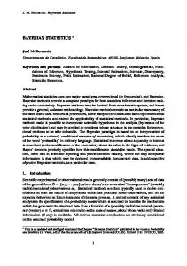
otherwise set (i) (i−1) (i−1) n(i), X 0:n , X 0:n (i −1) . (i ) = n 6. If iq0.95] = 57 [ES − 2σˆ T , ES + 2σˆ T ] [ES − 2σˆ T , ES + 2σˆ T ] D0=[42,142] = [25.0, 64.4] = [41.6, 62.8] In Figure IV we provide analysis of the mixing of the trans-dimensional sampler by considering the proportion of samples from the chain which were of length 1, which is used in the estimation of cˆ opt . We present these results as a function of the length of the chain N, for several different points at which we evaluate the annual loss distribution, x=10, 50, 200. It is clear from these sample paths that as the distance from the origin, at which we choose to evaluate our annual loss distribution fY(x) increases, the length of chain N required before this estimate stabilizes will increase. 0.5
14
We also note that the error in the approximation due to forming a piecewise linear approximation of the annual loss distribution is not accounted for in the calculation of σˆ . However, we know from the Central Limit Theorem that providing that the variance is finite the value of σˆ will → 0 as the number of importance samples N → ∞ [Kipnis & Varadhan,1986], for any given grid spacing. This does not however ensure our estimate of the quantile is consistent, only that the actual estimates of the annual loss distribution are asymptotically correct at the locations for which we place our grid points. However, as we can control this granularity, we can make this as accurate as we desire. Standard results may be used to bound the additional error introduced by this numerical integration stage [Robert & Casella, 2004]. Additionally, we have not accounted for error associated
20
with the fitting procedure to estimate the parameters of the severity and frequency distributions, this is future work. Figure IV: Proportion of time n=1 versus length of chain N as a function of x.
4.1.2) Computational Considerations. To compare the computation time, we consider two evaluations. The first is the time taken to obtain a single point estimate of the annual loss distribution, for roughly the same accuracy. The second is the computation time for expected shortfall. Note we have not made use of the fact that we can easily parallelize our computation, reducing the simulation time significantly for Algorithm 1 and Algorithm 2. All simulations were implemented in Matlab and performed on an Intel Core 2 Duo processor (2.4GHz) with 4GB RAM. Table II: Comparison of Computation Time Algorithm Computation of fY (10) Basic Monte Carlo N=50mil ∼ 171 min Standard Importance ∼ 0.1 min (N=10k, NT=100k) Sampling Algorithm 1 ∼ 0.6 min (N=50k, NT=500k) * M samples: fY (x = 10) ∼ 1 min (N=100k, NT=1000k) * N samples per grid point: ∼ 4.9 min (N=500k, NT=5000k) E[Y|Y>q0.95] Optimal Importance ∼ 2 min (N=10k, NT=60k) Sampling Algorithm 2 ∼ 3.5 min (N=50k, NT=100k) * N samples + (50k burn∼ 5.3 min (N=100k, NT=150k) in): ∼ 20.5 min (N=500k, NT=550k) fY (10) * N samples+(100k burn-in) per grid point: E[Y|Y>q0.95]
E[Y|Y>q0.95]
∼ 171 min N=50k per grid point {42,43…,142} ∼ 45 min (N=50k, NT=100k)
N=50k +(100k burn-in) NT=150k per grid point {42,43…,142} ∼13hrs (serial processing) N=50k +(100k burn-in) NT=150k per grid point-{42,43…,142} ∼ (100/3)*5.3 ≈ 171 min (parallel processing 3 CPUs) Table II demonstrates that the computational cost of using standard importance sampling under Algorithm 1 is a significant improvement in computation time compared to basic Monte Carlo. For more complex evaluation scenarios simple Monte Carlo will be unable 21
to provide solutions for a reasonable computational cost. Additionally, Algorithm 1 relies upon the simple importance distribution matching the target distribution reasonably well; if the function g is sharply peaked then this is unlikely to be the case and in such situations Algorithm 2 should remain an effective and efficient means of evaluating the quantities of interest at a fixed computational cost. It is clear that evaluation of the annual loss distribution at a fixed point x >> mode of fY when using the fixed importance sampling distribution, Algorithm 1, will degrade in performance as the function g becomes more peaked and hence the distance between x and the peak of g increases. This can be understood since if the importance distribution remains unchanged, then as the annual loss distribution becomes more peaked as a consequence of g becoming more peaked, relative to the importance sampling distribution, then the performance of such an importance sampling distribution will degrade in accuracy and variance. In these scenarios the optimal importance sampling distribution will be important. What is not so clear is how the performance of each algorithm compares if evaluating the annual loss distribution at different x values as g changes shape. We conclude by demonstrating in Figure V that the performance of MCMC importance sampling algorithm also significantly outperforms the standard importance sampler in these circumstances. To demonstrate this we present analysis of the impact of the shape of the severity distribution on the variance estimate obtained from each technique when performing evaluation of fY (x m ), where x m = max(1, arg max[g ( x )]) = max(1, arg max[ p1 f X ( x )]) . We only alter the parameters of the severity distribution and N for the standard importance sampling from Algorithm 1. Note, we do not change Pd since in practice, a good value for Pd will not be known a priori. We can then demonstrate that this is one of the advantages of trans-dimensional sampling since in Algorithm 2 popt(n) is “discovered” by the sampler on-line.
22
Overall, the results we obtained from using Algorithms 1&2, demonstrate that they work well. We show that unless one knows a priori that the function g is highly peaked, we advocate the use of the standard importance sampler as it is significantly faster and able to perform well. Only in more complex scenarios, if the standard importance sampler is producing variance in estimates which are not tolerable, should one then consider the trans-dimensional MCMC approach as a variance reduction technique. 4.2) Example 2: Poisson-GB2 compound process. Utilizing the analysis and subsequent advocated advice from example 1, we now build a more sophisticated model based on work presented in [Peters et al. 2006]. We develop a Poisson-GB2 compound process, Poisson(λ) frequency and GB2(a,b,p,q) severity distribution. We demonstrate that we again obtain accurate estimates of the annual loss distribution when compared to basic Monte Carlo if using Algorithm 1 as recommended from the analysis presented in Example 1 with significantly less computation time.
The flexibility of the GB2 distribution lies in the fact that it encompasses a family of distributions. Depending on the parameter values fitted using the loss data one can recover a range of parametric severity distributions with a flexible range of location, scale, skewness and kurtosis. We refer the reader to [Dutta et al. 2006, Peters et al. 2006] for discussion on the merits and properties of the GB2 distribution when used to model the severity distribution in an LDA framework. The GB2 distribution has density function given by a x ap−1 f (x ) = I 0,∞ (x ) , a p +q ( ) ap b B(p,q) 1+ (x /b)
[
]
(17)
where B(p,q) is the Beta function and the parameters a, p and q control the shape of the distribution and b is the scale parameter. For discussion of how the parameters are interpreted in terms of location, scale and shape see [Dutta et al. 2006]. It was demonstrated in [Bookstaber et al, 1987] that the GB2 distribution (17) encapsulates many different classes of distribution for certain limits on the parameter set. These include the lognormal ( a → 0 , q → ∞ ), log Cauchy ( a → 0 ) and Weibull/Gamma ( q → ∞ ) distributions, all of which are important severity distributions used in operational risk models in practice. Here we consider the parameter values for the GB2 family corresponding to the Lomax distribution (Pareto distribution of the 2nd kind or Johnson Type VI distribution) with parameters [a, b, p, q] = [1, b, 1, q], which when reparameterized in terms of q > 0, λ > 0 and x > 0, is given by −(q +1) q⎛ x⎞ . (18) h (x;α ,b) = ⎜1+ ⎟ b⎝
b⎠
The heavy-tailed Lomax distribution has shape parameter q and scale parameter b. Next we present three sets of analysis using our approach for a range of parameter values [a, b, p, q,λ].
23
The first analysis in Figure VI demonstrates the basic Monte Carlo versus the standard importance sampling procedure as a function of the number of importance samples N (=100,500,1k,10k). Demonstrating that as the number of importance samples increases, the accuracy improves as expected, we also include simulation time for the entire distribution on [0,100] in the figure. Figure VI: Analysis of Annual Loss Distribution Estimate vs N(number of I.S. samples).
The second analysis in Figure VII demonstrates, the performance as a function of λ(=0.01,1,10), note each plot also contains simulation time for each approach. In this example we use approximately the smallest N found to provide acceptable accuracy. Clearly this analysis demonstrates two points, our approach is highly accurate for a range of mean frequencies and secondly the computational time savings using our approach are significant. In the case in which λ=0.01 the basic Monte Carlo would require more than N>50mil to obtain the same accuracy obtained by our approach as x increases. Figure VII: Analysis of Annual Loss Distribution Estimate vs λ (mean of frequency distribution).
24
The third analysis in Figure VIII demonstrates the performance as a function of α(=q) (=0.1,1,10), the shape parameter of the severity distribution. Figure VIII: Analysis of Annual Loss Distribution Estimate vs q (shape of the severity distribution).
5) Discussion In this article, we have introduced new methodology to the simulation of annual loss distributions under an LDA framework for Operational Risk. We have demonstrated their performance on some real practical problems and compared with standard industry practices. We advocate that practitioners adopt these techniques as they can significantly improve performance for a given computational time budget. Furthermore, correlation between different Business unit/Risk types can be introduced under our approach in the usual manner used in financial institutions, via the use of Copula transforms in an LDA framework. In such settings, one could sample from each constructed annual loss distribution and apply a copula transform to these samples to obtain correlation at the annual loss level. Future work will consider developing a richer class of trans-dimensional Markov Chain Monte Carlo moves to reduce the computational effort when using minimum variance estimates. One could also consider extending such approaches to allow for introduction of correlation between severity and frequency during the simulation process. It would also be interesting to compare the performance of the algorithms discussed here when applied to more challenging distributions.
6) Acknowledgements The first author is supported jointly by an Australian Postgraduate Award, through the Department of Statistics at UNSW and a top-up research scholarship through CSIRO Quantitative Risk Management. Thank you goes to Pavel Shevchenko, Xiaolin Luo, Jerzy Sawa and Matthew Delasey for useful discussions. 25
References 1. Baker C. (2000). Volterra Integral Equations, Numerical Analysis Report No. 366, Manchester Centre for Computational Mathematics Numerical Analysis Reports. 2. Baker C. (1977). The Numerical Treatment of Integral Equations, Oxford Clarendon Press. 3. Bartolucci F., Scaccia L. and Mira A. (2006) Efficient Bayes factor estimation from the reversible jump output, Biometrika, 93(1), 41-52. 4. Bookstaber R. and J. McDonald (1987). A general distribution for describing security price returns. The Journal of Business, 60 (3), 401-424. 5. Brooks S., Giudici P. and Roberts G. (2003). Efficient Construction of Reversible Jump MCMC Proposal Distributions (with discussion), Journal of the Royal Statistical Society, Series B, 65, 3-55. 6. Chavez-Demoulin V., Embrechts P. and Neslehova J. (2006). Quantitative Models for Operational Risk: Extremes, Dependence and Aggregation. Journal of Banking and Finance, 30(10), 2635-2658. 7. Cruz M. (2002). Modelling, Measuring and Hedging Operational Risk. John Wiley & Sons, Chapter 4. 8. Devroye L. (1986). Non-Uniform Random Variate Generation. Springer-Verlag, New York. 9. Doucet A. and Tadic V. (2007). On Solving Integral Equations using Markov Chain Monte Carlo, Technical Report CUED-F-INFENG Cambridge University no. 444. 10. Doucet A., de Freitas N. and Gordon, N. (2001). Sequential Monte Carlo Methods in Practice. Springer-Verlag, New York. 11. Dutta K. and J. Perry (2006). A tale of tails: An empirical analysis of loss distribution models for estimating operational risk capital. Federal Reserve Bank of Boston, Working Papers No. 06-13. 12. Embrechts P., H. Furrer and R. Kaufmann (2003). Quantifying regulatory capital for operational risk. Derivatives Use, Trading & Regulation, 9 (3), 217—223. 13. Gelman A., J. B. Carlin, H.S. Stern and D.B. Rubin (1995). Bayesian Data Analysis. Chapman and Hall. 14. Gilks W., S. Richardson and D. Spiegelhalter (1996). Markov Chain Monte Carlo in Practice. Chapman and Hall. 15. Glasserman, P. (2003). Monte Carlo Methods in Financial Engineering. Springer. 16. Green P. (1995). Reversible Jump Markov Chain Monte Carlo Computation and Bayesian Model Determination, Biometrika, 82, 711-732. 17. Green P. (2003). Trans-dimensional Markov Chain Monte Carlo, chapter from Highly Structured Stochastic Systems, Oxford University Press. 18. Kipnis, C. and Varadhan, S. R. S. (1986). Central limit theorem for additive functionals of reversible Markov processes and applications to simple exclusions. Communications in Mathematical Physics, 104, 1—19. 19. Klugman, S. Panjer, H. and Willmot, G. (2004). Loss Models: From Data to Decisions. John Wilely, New York. 20. Linz P. (1987). Analytical and Numerical Methods for Volterra Equations, Mathematics of Computation, 48, No. 178, 841-842 26
21. Menn C. (2006). Calibrated FFT-based Density Approximation for alpha-stable Distributions. Computational Statistics and Data Analysis, 50, 8, 1891-1904. 22. Meyn S. and R. Tweedie (1993). Markov Chains and Stochastic Stability, Springer. 23. Neslehova J, Embrechts P. and Chavez-Demoulin V. (2006). Infinite Mean Models and the LDA for Operational Risk. Journal of Operational Risk, 1(1), 325. 24. Orsi A. (1996). Product Integration for Volterra Integral Equations of the Second Kind with Weakly Singular Kernels, Mathematics of Computation, 65, No. 215, 1201-1212 25. Panjer H. (2006). Operational Risk: Modeling Analytics, Wiley. 26. Panjer H. and Wilmott G. (1992), Insurance Risk Models, Chicago Society of Actuaries. 27. Panjer H. (1981). Recursive Evaluation of a Family of Compound Distributions, Astin Bulletin 12, 22-26. 28. Peters G. and Teruads V. (2007). Low Probability Large Consequence Events. Australian Centre of Excellence for Risk Analysis, Project No. 06/02. 29. Peters G. and Sisson S. (2006). Bayesian Inference Monte Carlo Sampling and Operational Risk. Journal Of Operational Risk, 1, No. 3. 30. Robert C.P. and Casella G. (2004). Monte Carlo Statistical Methods, 2nd Edition. Springer Texts in Statistics. 31. Rotar, V. (2007). Actuarial Models – The Mathematics of Insurance. Chapman & Hall CRC. 32. Shevchenko, P. and M. Wuthrich (2006). The structural modelling of operational risk via Bayesian inference: Combining loss data with expert opinions. CSIRO Technical Report Series, CMIS Call Number 2371. 33. Sisson, S. (2005). Trans-dimensional Markov Chains: A Decade of Progress and Future Perspectives. Journal Of American Statistical Association, 100, 10771089. 34. Stroter, B. (1984). The Numerical Evaluation of the Aggregate Claim Density Function via Integral Equations. Blatter der Deutschen Gesellschaft fur Versicherungs-mathematik, 17, 1-14. 35. Sundt, B and Jewel, W. (1981). Further Results on Recursive Evaluation of Compound Distributions. Astin Bulletin, 12, 27-39. 36. Willmot, G. and Panjer, H. (1985). Difference Equation Approaches in Evaluation of Compound Distributions. Insurance: Mathematics and Economics, 6, 195-202. 37. Willmot, G. (1986). Mixed Compound Poisson Distributions. Astin Bulletin, 16, S, S59-S79.
27