Author manuscript, published in "Natural Hazards and Earth Systems Sciences, 9 (2009) 15 p."
Bayesian stochastic modeling of a spherical rock bouncing on a coarse soil Franck Bourrier1, Nicolas Eckert1, François Nicot1, and Félix Darve2
[1] Cemagref - UR ETNA - 2, rue de la Papeterie - BP 76 - 38 402 Saint Martin d’Hères Cedex France [2] L3S-R - INPG, UJF, CNRS - Domaine Universitaire – BP 53 -38 041 Grenoble Cedex 9 France
hal-00456156, version 1 - 12 Feb 2010
Correspondence to: F. Bourrier (
[email protected])
Abstract: Trajectory analysis models are increasingly used for rockfall hazard mapping. However, classical approaches only partially account for the variability of the trajectories. In this paper, a general formulation using a Taylor series expansion is proposed for the quantification of the relative importance of the different processes that explain the variability of the reflected velocity vector after bouncing. A stochastic bouncing model is obtained using a statistical analysis of a large numerical data set. Estimation is performed using hierarchical Bayesian modeling schemes. The model introduces information on the coupling of the reflected and incident velocity vectors, which satisfactorily expresses the mechanisms associated with boulder bouncing. The approach proposed is detailed in the case of the impact of a spherical boulder on a coarse soil, with special focus on the influence of soil particles’ geometrical configuration near the impact point and kinematic parameters of the rock before bouncing. The results show that a firstorder expansion is sufficient for the case studied and emphasize the predominant role of the local soil properties on the reflected velocity vector’s variability. The proposed model is compared with classical approaches and the interest for rockfall hazard assessment of reliable stochastic bouncing models in trajectory simulations is illustrated with a simple case study.
Key words: Rockfall, Hazard, Trajectory analysis, Bouncing, Impact, Discrete Element Method, Hierarchical Bayesian Modeling.
1
1.
Introduction
Trajectory simulation models classically use Digital Elevation Models that define the topography, and geographic information systems that provide information on the rockfall sources and the spatial distribution of the parameters necessary to calculate the bouncing of the falling rocks at each point of the study site. The models classically used for bouncing calculations are based on restitution coefficients that express the dependence of the kinematic parameters of the rock after impact (reflected kinematic parameters) on the kinematic parameters of the rock before impact (incident kinematic parameters). However, experimental studies have proved the complexity of simulating this dependence by means of reasonably simple mechanical models (Wu, 1985; Bozzolo and Pamini, 1986; Chau et al., 1998; Ushiro et al., 2000; Chau et al., 2002;
hal-00456156, version 1 - 12 Feb 2010
Heidenreich, 2004). In addition, deterministic prediction of boulder bouncing remains highly speculative because the available information on the mechanical and geometrical properties of the soil and the boulder is not sufficient. Indeed, the spatial distributions of the parameters of the bouncing model integrated into the geographic information system result from a field survey which, for practical reasons, cannot be exhaustive. Moreover, as for many physical processes in the field of natural hazards, it seems impossible to predict the bouncing deterministically. Stochastic bouncing models have therefore been proposed to integrate most of the sources explaining the bouncing phenomenon’s variability using statistical laws (Paronuzzi, 1989; Pfeiffer and Bowen,1989; Azzoni et al., 1995; Dudt and Heidenreich, 2001; Guzzetti et al., 2002; Agliardi and Crosta, 2003). The variability sources can be divided into those associated with the soil properties (soil surface, porosity, particle size and shape, etc.) and those related to the incident conditions (incident kinematic parameters, boulder size, shape and orientation, etc.) (Pfeiffer and Bowen, 1989; Labiouse, 1999). Although an important step further, these approaches require a thorough calibration of the statistical laws using large data sets. Real rockfall events or field experiments are not directly usable for this purpose because either the data set is incomplete (rockfall events) or reproducible impact conditions are difficult to obtain (field experiments). Taking inspiration from other research fields such as hydrology (Rao, 1996; Perreault et al., 2000a; Perreault et al., 2000b) and avalanche science (Eckert et al., 2007; Eckert et al., 2008) in which dealing with stochasticity is more common, this paper aims at defining a bouncing model explicitly distinguishing these different sources of variability. In section 2, a general framework that aims at determining the kinematics of the boulder after bouncing from the kinematics before bouncing using a stochastic operator and its related Taylor 2
series expansion is presented first. This section also shows how the stochastic operator can be characterized using a Bayesian statistical analysis (Wickle, 2003; Clark, 2005) of numerical simulations. The study focuses on the impact of a boulder on a coarse soil, which is common in the context of rockfall trajectory analysis. In a first approximation, only the influences of the incident kinematic parameters and the soil particle configuration near the impact point of a spherical boulder are studied. In section 3, the stochastic bouncing model obtained using this approach is presented and discussed in detail. An extensive sensitivity analysis is performed to evaluate the bouncing model’s range of validity. Section 4 discusses the advantages and limitations of our approach with regard to classical approaches. The usefulness of using this stochastic bouncing model for the prediction of rockfall hazard is finally illustrated through a
hal-00456156, version 1 - 12 Feb 2010
simple case study. 2.
Materials and methods
2.1.
Stochastic modeling of the impact
The bouncing model is developed in a two-dimensional frame, which is classical in the field of trajectory analysis (Guzzeti et al., 2002; Dorren et al., 2004). A generalized velocity vector V composed of a normal-to-soil-surface velocity component v y , a tangential-to-soil-surface velocity component v x – both expressed at the gravity center of the falling rock – and a rotational velocity ω properly describes the kinematic parameters of the boulder: V = (v x
vy
Rbω )
t
(1)
where Rb is the mean radius of the boulder. For given mechanical and geometrical properties of the boulder and the soil, it is assumed that the incident V in and reflected V re generalized velocity vectors of the boulder can be related by ~ a stochastic operator f : ~ V re = f (V in )
(2)
~ The formulation of the operator f should express the complexity of the mechanisms leading to the dependence of the reflected velocity vector to the incident velocity vector. It should also be relevant for the variability of the bouncing process depending on the variability of the soil properties and the incident kinematic parameters.
3
~ Assuming that a Taylor series expansion of the operator f with respect to all components of the incident velocity vector V in exists, the operator Α composed of the coefficients of the n -order ~ Taylor series expansion of f is defined. The operator Α associates the reflected velocity vector V re with an incident velocity vector expressed as T in :
V re = AT in + R
(3)
hal-00456156, version 1 - 12 Feb 2010
with 1 a100 2 Α = a100 3 a100
1 1 a010 ... auvw ... a10 n 0
Tin = vxin
viny
2 2 a010 ... auvw ... a02n 0 3 3 a010 ... auvw ... a03n 0
1 a00 n 2 a00 n , 3 a00 n
... (vxin )u (v iny )v ( Rb win ) w ... (v iny ) n
t
( Rb win ) n , u ∈ [1, n] , v ∈ [1, n ] , w ∈ [1, n] ,
~ and R a remainder term denoting the difference between the operator f and its n-order Taylor series expansion. The number of the incident vector T in component is equal to 3 for a first-order ~ ~ Taylor series expansion of f , 7 for a second-order Taylor series expansion of f , etc. One can ~ note that, for a first-order Taylor series expansion of the operator f , the incident vector T in is equal to the incident velocity vector V in . The high variability of the local configurations of the soil and the incident kinematic conditions induces the operator Α and the remainder term R to take very different values. This suggests adopting a stochastic approach distinguishing the variability associated with both the operator Α and the remainder term R . Note that this paper only investigates in detail the case of the impact of a spherical boulder on a coarse soil. In a first approximation, the sources of variability considered are limited to the incident kinematic parameters and the soil particles’ geometrical configurations. However, the proposed framework is very general and could be applied to modeling boulder bouncing for impacts on different soil types and for different boulder mechanical and geometrical properties. Indeed, as exemplified in this paper, it allows extracting the respective contribution of the different sources of variability using Bayesian inference.
2.2.
Data set definition from numerical simulations
The large data sets needed for statistical analyses can be obtained from numerical simulations of impacts. Additionally, in the simulations, the influences of the geometrical configuration of the soil near the impact point and the incident kinematic parameters can be explored separately, since a precise and reproducible definition of these parameters is possible.
4
2.2.1.
Numerical modeling of impacts using the Discrete Element Method
Assuming that rocks composing the coarse soil can be considered as rigid locally deformable two-dimensional bodies, the software Particle Flow Code 2D (Itasca, 1999) based on the Discrete Element Method (Cundall and Strack, 1979) is used. In the Discrete Element Method (DEM), particles are subjected to gravitational forces and to contact forces. Contact forces are applied to neighboring particles in contact. For a given time step, once gravitational and contact forces have been computed, the translational and rotational velocities of the particles are determined by solving the balance equation using an explicit solving scheme. The resulting particle displacements are used to update particle locations for the next time step. In this study, the contact forces acting between particles are calculated using the Hertz-Mindlin model
hal-00456156, version 1 - 12 Feb 2010
(Mindlin and Deresiewicz, 1953). Contact forces are governed by three parameters set at classical values for rocks (Goodman, 1980): the shear modulus G is set at 40 GPa, the value of the Poisson ratio ν is set at 0.25 and the local friction angle φ is 30°. In addition, the density ρ of the boulder and the soil particles is set at 2650 kg/m3. This contact model takes frictional processes between adjoining particles into account. Other dissipation sources also exist within real granular soils subjected to dynamical loadings, such as local yielding near the contact surface, crack propagation, and rock breakage. However, in the context of the simulations where a boulder is approximately of the same size as the soil particles, other dissipation sources can be assumed to be negligible compared to frictional dissipation in a first approximation (Oger et al., 2005; Bourrier et al., 2008a). The mean radius of the soil particles is Rm = 0.3 m. Given that natural scree are polydisperse granular assemblies (Kirkby and Statham, 1975), the ratio between the mass of the soil’s smaller particles and larger particles is set at 10. In the case of an impact on a coarse granular soil, boulder and soil particle sizes are nearly the same. The boulder radius Rb varies from Rm to 5Rm. The influence of particle shape is also explored by defining two different soil samples composed of either spherical particles or elongated particles modeled by indivisible assemblies of spherical particles called clump particles, which can realistically model the shape of soil rocks (Bertrand et al. 2006; Deluzarche and Cambou 2006, Bourrier et al. 2008a). The soil sample generation procedure leads to soil porosity values of 0.204 for spherical particles and 0.171 for clump particles. Additional details on the soil properties can be found in Bourrier et al. (2008a). Although simulation results also depend on soil sample depth and porosity (Bourrier et al. 2008a), the influence of these parameters is not investigated in a preliminary approximation. Soil sample depth is set at 12Rm. Analyses of the influence of the model parameters on the impact 5
simulations (Bourrier et al., 2008a) have shown that, for a soil depth corresponding to classical values in the field of rockfall simulations, the bouncing of the boulder mainly depends on the ratio between the boulder radius Rb and the mean radius of a soil particle Rm, the shape of the particles, the incident kinematic parameters and the geometrical configuration of the soil particles near the impact point. We will focus on modeling the variability associated with the incident kinematic parameters and the geometrical configuration of the soil particles near the impact point using a stochastic bouncing model (see section 3). In addition, the influence of the ratio of the boulder radius Rb to the mean radius of a soil particle Rm and the shape of the particles on the parameters on the stochastic bouncing model will also be investigated in section 3 by means of sensitivity analyses. Once the soil sample is generated, impact simulations are run for varying impact points and
hal-00456156, version 1 - 12 Feb 2010
incident kinematic parameters. The location of each impact point is defined very precisely. In addition, incident kinematic conditions are fully determined by the magnitude of the incident velocity Vin, the incident angle αin and the incident rotational velocity ωin (Figure 1). These parameters are directly related to the normal and tangential velocity components by: v xin = V in sin(α in )
(4)
v iny = −V in cos(α in )
(5)
Finally, reflected velocities are collected when the normal component of the boulder velocity reaches its maximum, which corresponds to the last contact between the soil and the boulder.
Figure 1 It is important to note that the relevance of the numerical model has been proved by comparing its results to the available literature (Bourrier et al., 2008a) and to half-scale experiments of impacts on a coarse soil (Bourrier et al., 2008b). In particular, the impact model was calibrated and validated using laboratory experiments of the impact of a 10-cm spherical rock on a coarse soil composed of gravels ranging from 1 cm to 5 cm (Bourrier et al., 2009; Bourrier et al., 2008b). The incident velocity of the projectile was 6 m/s and the incident angle could reach values from 0° to 75°. Satisfactory agreement between the laboratory experiments and the numerical simulations of impacts proves that the stochastic impact model adequately expresses the energy transfers occurring during the impact of a boulder on a coarse soil. One limitation could stem from the differences in the sizes of the impacting and soil rocks during calibration and during application in this study. However, the influence of scale change effects was proved to be small by comparing the results of the numerical simulations of impacts at 6
different scales (Bourrier, 2008). This has been confirmed by results from the literature in the field of aeolian sand transport (Oger et al., 2005).
2.2.2. Numerical simulation campaign For given soil and boulder properties, several impact simulations were conducted for varying impact points and incident kinematic parameters. As stated above, the only sources of variability accounted for are the incident kinematic parameters and the soil particle geometrical configuration near the impact point. In addition, the dependency of the stochastic bouncing model parameter values on the boulder size and soil particle shape will be explored in section 3.3. Other impact model parameters are set at fixed values: the mechanical properties of the
hal-00456156, version 1 - 12 Feb 2010
particles (G, ν, φ, ρ), the porosity and grading curve of the soil sample and the boulder size are fixed parameters. Impact points are first precisely defined so that the same impact point can be used for several incident kinematic conditions: for a given impact point, a set of equally distributed incident kinematic parameters is explored. Kinematic parameter values range within the limits defined from rockfall events (Azzoni et al., 1992). For each impact point, all combinations of the chosen values for incident kinematic parameters (Table 1) are explored. Preliminary numerical investigations have shown that a minimum of P = 100 impact points has to be chosen to ensure that the mean values and standard deviations of the reflected velocity components (Bourrier et al., 2007) have reached their asymptotic value corresponding to the value obtained for very large numbers of impact points.
Table 1
2.3.
Stochastic analysis of simulation results based on Bayesian inference
2.3.1. Hierarchical stochastic modeling ~ First, at each impact point p ∈ [1, P ] , the Taylor series expansion (Eq. (3)) of the operator f defined in Eq. (2) is considered a linear regression of the reflected velocity vector V re with regard to the incident vector T in :
7
re Vpk ~N 3 ( Α p Tpkin , Σ)
(6)
re The reflected velocity Vpk is thus sampled from a local three-dimensional Gaussian vector fully
defined by its local mean vector Α p Tpkin varying from one impact event to another and its covariance matrix Σ , which is constant for all incident kinematic conditions k ∈ [1, K ] and impact points (homoscedascity assumption). The vector Α p Tpkin is the mean predictor in the ~ linear regression. Its variability quantifies the variability of the Taylor series expansion of f , while the covariance matrix Σ accounts for the variability of the remainder term R . Our stochastic model is therefore based on the assumption that the variability of the operator Α is
hal-00456156, version 1 - 12 Feb 2010
only related with the variability of the soil particles’ geometrical configuration, whereas the remainder term R is associated with all other variability sources accounted for in the impact model, for instance random uncertainties that are not modeled explicitly. The realism of the mechanical modeling representing the coupling between the reflected and incident velocity vector depends on the order of the Taylor series expansion. For convenience, the matrix Α p is rewritten 1 Α lp = a100 p
as 1 a010 p
1 ... auvw p
a
vector
... a01 n 0 p
a100 n p
having
2 2 a100 ... a00 np p
N 3 3 a100 ... a00 np , p
components with
1→3 auvw
denoting the coefficients of the matrix A defined in Eq (3) at the point p ∈ [1, P ] . The number N=(n+1)(n+2)(n+3)/2−3 of the vector’s coefficients is equal to 9 for a first-order Taylor series ~ ~ expansion of f (n = 1) , 27 for a second-order Taylor series expansion of f (n = 2) , etc. Second, it is assumed that the results observed at the different impact points are, in some ways, similar because the macroscopic properties of the soil (porosity, the particles’ mechanical properties, grading curve, etc.) are the same. This makes us use hierarchical modeling to allow information to be partially shared between the different impact points and to extract the common patterns in all samples. For all impact points p , the coefficients of the operator Α p are therefore assumed to be realizations of the same Gaussian vector such as:
A1p ~NN (M a , Σ a )
(7)
M a and Σ a are the mean vector and the covariance matrix of the N-dimensional Gaussian vector. M a models the mean behavior all over the different local soil particles’ geometrical
8
configurations, whereas the variability of Α lp measured by Σ a expresses how close the different reflected velocities at the different impact points are. Note that with a non hierarchical model only two extreme cases could have been considered: i) all samples are identically distributed, with the same operator A p for all impact points, or ii) the different samples are so different that they have to be modeled by independent distributions. On the contrary, even if it complicates model specification and inference, the hierarchical structure allows a comprehensive exploration of the grey zone situated between these two extreme cases. This makes each local estimation more robust and allows the overall quantities M a and Σ a to be captured.
hal-00456156, version 1 - 12 Feb 2010
The analytical formulation of the model developed can be summarized as follows. First, the analytical expression of p (Vpkre A p , Tpkin , Σ) , the probability of the observed reflected vector V pkre in is: knowing the values of A p , Σ and the observed incident kinematic conditions Tpk
p(V
re pk
1 re in t −1 re in − ( Vpk − A p Tpk ) Σ ( V pk − A p Tpk ) 1 2 A p , T , Σ) = e (2π )3/ 2 det( Σ )1/ 2
(8)
in pk
Second, the analytical expression of the probability p ( Α lp M a , Σ a ) of the nonobserved latent vector Α lp knowing the values of M a , Σ a is: 1 − ( Α lp − M a )t Σ a 1 p( Α M , Σ ) = e 2 (2π ) N / 2 det( Σ a )1/ 2 l p
a
a
−1
( Α lp − M a )
(9)
The unknown parameters of the stochastic model are M a , Σ a , Σ and the data are V pkre and Tpkin . The latent quantities Α lp with p ∈ [1, P ] have a hybrid status: with regard to the data V pkre they are parameters and therefore must be estimated, whereas they behave as data with regard to parameters M a and Σ a . Figure 2 gives a general overview of the model using a direct acyclic graph (DAG), which expresses conditional dependence. Circled nodes represent stochastic variables, while rectangles indicate observed values and diamonds model parameters. The DAG
9
clearly illustrates the three layers distinguished in our approach: impact that depends both on incident velocity and location, local soil configuration and the soil’s global parameters.
Figure 2
2.3.2.
Bayesian inference
Due to its hierarchical nature, determining the parameters of our stochastic model using a classical statistical approach (Fischer, 1934; Neyman and Pearson, 1933) is tricky. On the other hand, estimates for the parameters M a , Σ a and Σ and latent vectors Α lp , p ∈ [1, P ] can be
hal-00456156, version 1 - 12 Feb 2010
more easily obtained using Bayesian inference (Bayes, 1763). The result of applying the Bayes theorem is p ( Α lp , M a , Σ a , Σ Vpkre , Tpkin ) , the joint posterior probability distribution of all model in unknowns knowing the data V pkre and Tpk :
(10)
p( Α lp , M a , Σ a , Σ Vpkre , Tpkin ) = 1
χ
p(M a , Σ a , Σ) × p(Vpkre A p , Tpkin , Σ) × p ( Α lp M a , Σa )
The determination of p ( Α lp , M a , Σ a , Σ Vpkre , Tpkin ) therefore requires the probability of the reflected vector V pkre knowing the data, latent variables Α lp and the overall parameter Σ ( p (Vpkre A p , Tpkin , Σ) ) and the probability p ( Α lp M a , Σ a ) of the latent variables given the data and the overall parameters M a , Σ a . Both of them are fully defined by the hierarchical model detailed in section 2.3.1. Moreover, determining p ( Α lp , M a , Σ a , Σ Vpkre , Tpkin ) also requires specifying p (M a , Σ a , Σ ) .
χ = ∫ p (M a , Σ a , Σ) × p (Vpkre A p , Tpkin , Σ) × p ( Α lp M a , Σ a )dM a dΣ a dΣ
is
a
normalizing constant that does not depend on the problem’s unknowns, but makes all difficulty of Bayesian inference (see section 2.3.3). According to Bayesian interpretation, p (M a , Σ a , Σ) is a prior, which is a probability distribution function that expresses the expertise about the parameters that is available before the 10
data analysis. To respond to the classical objections to use such prior information, in this paper we use poorly informative priors (Box and Tiao, 1973) that lead asymptotically to the same estimators as classical approaches (Berger, 1985). To facilitate inference using Gibbs sampling (see section 2.3.3), the chosen poorly informative priors have been taken from conjugate families (see Gelman et al., 1995): a normal Gaussian vector with a null mean and very large variance for M a , and Wishart distributions with low degrees of freedom for the inverse of the covariance matrixes ( Σ, Σ a ) . Taking very poorly informative priors is possible since a data set as large as necessary is available given that numerical simulations were used to generate it. Poorly informative priors have the advantage of letting the data speak for themselves so as to infer
hal-00456156, version 1 - 12 Feb 2010
parameters with as much physical meaning as possible. Note finally that, contrary to classical statistical approaches, Bayesian inference provides a probability distribution rather than a point estimate associated with a confidence interval for each unknown quantity. For applications, the mean of the posterior distribution and the 95% credible interval [q 2.5 , q97.5 ] are generally chosen for each unknown parameter, which represents the best prediction given the data and the related uncertainty. In this paper, this convention has been followed. In addition, the coefficient of variation cv defined as the ratio between the standard deviation and the mean value of the posterior distribution is also provided. It is a normalized measure of the dispersion of the posterior distributions but has to be interpreted with care for distributions with small mean values.
2.3.3. MCMC methods For hierarchical models, the computation of Bayes theorem is generally analytically unfeasible because of the problems calculating the normalizing constant χ . Today this limitation is routinely overcome, even for very complex models, with Monte Carlo techniques based on Markov chain properties (Brooks, 2003; Gilks et al., 2001). A general discussion of these Markov Chain Monte Carlo (MCMC) methods can be found in Robert and Casella (1998). Their aim is to obtain the posterior distribution of all model unknowns (parameters and latent variables) using an iterative procedure. Reasonable results can only be obtained if the algorithm is handled with care. In particular, one must ensure that the convergence is attained for all
11
unknown parameters. In most cases, this requires launching many simulations for varying initial states and performing tests to check that the Markov chain has reached the stationary regime. Depending on the model and the choice of priors, partial analytical computations can sometimes be performed for rather simple hierarchical models. This is the case for our model, given its fully Gaussian nature and the choice of conjugate priors for all parameters. However, the full analytical expression of the joint posterior distribution remains out of reach, so that recourse to a simulation procedure is unavoidable (see Gelman et al., 1995, chapter 15). It was therefore decided to perform a MCMC simulation for all unknowns, but to take advantage of the model’s structure by running the Gibbs sampler (Geman and Geman, 1984). This MCMC algorithm is based on the different full conditional distributions of one unknown (parameter and latent
hal-00456156, version 1 - 12 Feb 2010
variables) given the others, which can actually all be obtained with our model. The Gibbs sampler is particularly suitable because, when it can be run, it ensures a quick convergence with regard to the more general but less efficient Metropolis-Hastings algorithm (Metropolis et al., 1953). Note finally that, if the hierarchical structure is dropped by neglecting the random noise Σ , all computations can be performed analytically (see section 3.2 for discussion). For all the models tested (different orders of the Taylor series expansion), 20,000 iterations were performed with different chains starting at different points of the parameter space. The first 10,000 iterations were deleted to ensure that the ergotic state was attained. Convergence was checked for the second group of 10,000 iterations by comparing the distributions obtained with the different chains. A few marginal posterior distributions are shown in Figure 3 for the firstorder model detailed in section 3.2. For all parameters, the credibility intervals obtained are small (Table 2). It therefore appears that the information conveyed by the data is sufficient and only the mean values and therefore be used with confidence.
Figure 3
Table 2
12
2.3.4. Evaluation of model quality The quality of the model is first evaluated by estimating the fraction of the variability of the reflected velocities that is captured by the random variable ΑT in corresponding to the n-order ~ Taylor series expansion of f with regard to the total variability of the results. For the p th impact point, the s th component of the reflected velocity vector V re and varying incident conditions k , the ratio rps is calculated such that:
rps =
V ( A p Tpkin ( s ))
(11)
V ( A p Tpkin ( s )) + Σ( s, s )
hal-00456156, version 1 - 12 Feb 2010
in in where V ( A p T pk ( s )) denotes the variance of the s th component of the random variable ΑT for a
fixed impact point p and varying incident conditions k , whereas Σ( s, s ) denotes the s th diagonal term of the covariance matrix Σ . If rps = 100%, all the variability of the results is explained by the random variable ΑT in . To facilitate the comparison between the models evaluated, global indicators are calculated from the rps values, p ∈ [1, P ] . The mean r s of rps values is calculated to estimate a mean percentage of variability explained by the random variable ΑT in for each reflected velocity component. In addition, an overall ratio r is defined as the mean of all rps values.
3.
Application to the definition and evaluation of a stochastic bouncing model
In this section, the statistical analysis of the data set obtained from numerical simulations is performed using the above-described procedure. This analysis allows defining a stochastic bouncing model and performing a detailed study of this model. All results obtained in this section are valid in the case of the impact of a spherical boulder on a coarse soil. In addition, the results obtained depend on the assumptions related to the numerical model of the impact, the procedure used for the numerical simulation campaign, and the statistical analysis. The assumptions made during this analysis, the validity domain of the bouncing model obtained and the possible generalization of this model for practical purposes will be discussed in section 4.
13
3.1.
A first-order model is sufficient
Several models corresponding to increasing dimensions of the incident vector T in were compared to determine the final formulation of the stochastic bouncing model. Particular attention was given to the precision and concision criteria since the bouncing model must satisfy a compromise between a precise simulation of the impact phenomenon and a small dimension of the incident velocity vector T in . Table 3 summarizes the values of the r s and r ratios for different models corresponding to increasing dimensions of the incident vector T in in the case of the impact of a boulder with the radius set at Rb = Rm on a soil composed of spherical particles. The size of the data set used was
hal-00456156, version 1 - 12 Feb 2010
the same for all the models evaluated: 150 different incident kinematic conditions and 100 different impact points. The results first show that most of the variability of the reflected velocity is captured by the random variable ΑT in for all models used because the r s coefficients are all greater than 75%. Since all the models evaluated provide satisfying results in terms of precision, the most concise model was chosen: a dimension of T in equal to 3, explaining most of the variability of the results by the random variable ΑT in for a very small set of parameters. This model will hereafter be called the first-order stochastic bouncing model.
Table 3
3.2.
Detailed analysis of the first-order stochastic bouncing model
The model chosen corresponds to an incident vector T in composed of three components, which ~ is equivalent to a first-order Taylor series expansion of the stochastic operator f :
vxre a1 re 3 v y ~N ( a4 re a7 Rbω
a2 a5 a8
a3 vxin Σ xx a6 viny , Σ xy a9 Rbω in Σ xω
Σ xy Σ yy Σ yω
Σ xω Σ yω ) Σωω
where the coefficients a i are sampled from a nine-dimensional Gaussian vector:
14
(12)
a a m1a Σ11 ... Σ19 a1 ... ~N9 ( ... , ... ... ... ) a a m9a Σ19 a9 ... Σ 99
(13)
This model separates the sources of variability for the reflected velocity vector. The variability of parameters ai ( i ∈ [1, 9] ) is quantified by the covariance matrix Σ a . It is associated with the variations in the local soil properties. On the contrary, the variability quantified by the covariance matrix Σ is related to the remainder term R and is therefore mainly associated with the incident velocities. For the s th component of the reflected velocity vector, the standard deviation es = Σ ss of the
hal-00456156, version 1 - 12 Feb 2010
regression residuals provides a quantitative estimation of the proportion of the reflected velocity vector associated with the remainder term R . The correlations between two components s and t of the reflected velocity vector can be estimated by the linear correlation coefficient cst =
Σ st ∈ [ −1,1] . Σ ss Σtt
The estimates obtained show that, for all components of the reflected velocity vector, the standard deviation e s is smaller than 1 m/s. Second, all the linear correlation coefficients range within the interval [− 0.2,0.2] , which means that the correlations between the components of the reflected velocity are small. The analysis of the covariance matrix Σ indicates that the remainder ~ term R of the Taylor series expansion of f is negligible compared to the term ΑT in . The reflected quantities can therefore be correctly predicted using only the random variable ΑT in and omitting the covariance matrix Σ . The variability of the reflected velocity is then only associated with the variability of the soil’s local properties through the covariance matrix Σ a . It should be noted that, for future investigations on other simulated data sets, the model inference will be much easier, which will possibly make it accessible to practitioners who are not familiar with recent statistical developments. Indeed, ignoring the random noise Σ makes the model lose its hierarchical nature, so that the analytical expression of the posterior distribution is accessible if the conjugate priors are kept for M a and Σ a .
15
Finally, the variability associated with the operator Α is estimated using the marginal normal probability distribution functions of parameters a i (Figure 4). The estimates for their mean values mia and standard deviations sia = Σiia are provided in Table 4. Complementary to the marginal probability distribution functions of each parameter a i , the calculation of the linear correlation coefficients cija =
Σija Σija Σija
( i ∈ [1, 9] ; j ∈ [1,9] ) between the extra-diagonal terms of
matrix Σ a shows strong correlations between parameters a i because the cija values are large.
hal-00456156, version 1 - 12 Feb 2010
Figure 4
Table 4
3.3.
Sensitivity analysis
3.3.1. Methodology for comparing the model’s parameters To investigate the influence of several numerical simulation parameters, such as the number of impact points, the spatial distribution of soil particles, the value of the size ratio Rb/Rm and the shape of the soil particles, the parameters a i obtained for different values of these simulation parameters must be compared. The analysis is based on the marginal probability distribution functions of parameters a i summed up by their mean value mia and their standard deviation sia . Complementary to the qualitative comparison of the mean value mia and the standard deviation sia obtained in the different cases, a comparison criterion Ci is calculated for each parameter a i . The criterion Ci evaluates the difference between the marginal distribution of parameter airef obtained using reference conditions and the marginal distribution of parameter aicomp obtained using different numbers of impact points, different spatial distributions of the soil particles, different soil particle shapes or different boulder sizes. Criterion Ci is calculated as follows: 16
Ci =
P (bi − ≤ aicomp ≤ bi + ) − P (bi − ≤ airef ≤ bi + ) P (bi − ≤ airef ≤ bi + )
(14)
The lower bi − and upper bi + bounds are calculated such that P (bi − ≤ airef ≤ bi + ) = 95% and P (airef > bi + ) = 2.5% . Knowing the values of bi − and bi + makes it possible to determine the
probability P (bi − ≤ aicomp ≤ bi + ) . The reference conditions correspond to the impact of a spherical boulder with its radius set at Rb = Rm on a soil sample composed of spherical particles. The other properties of the soil sample are similar to those defined in section 2.2.1. For the reference conditions, impacts are simulated on 100 different impact points. Criterion Ci can be interpreted
hal-00456156, version 1 - 12 Feb 2010
as the difference between the most probable values of parameter ai encountered with the reference conditions and the conditions evaluated for which only one simulation parameter (number of impact points, soil sample geometrical configuration, soil particle shape, boulder radius) is changed compared to the reference conditions.
3.3.2. Robustness to simulation parameters The first aim of this analysis is to quantify the number of simulations necessary to obtain relevant values for parameters ai , which are therefore calculated using different numbers of impact points P for the same soil sample. The analysis of the results obtained shows that the simulation on P = 20 different impact points is sufficient to obtain stable values for the probability distribution functions of parameter a i . Indeed, all the values of criterion Ci are less than 10% if the number of impact points is higher than 20 (Table 5).
Table 5
The dependence of parameters a i on the spatial configuration of the soil sample particles is also evaluated. The model estimation is carried out for four different soils with the same grading curves, porosity and particle mechanical properties (G, ν, φ, ρ). The only difference between the four samples is the spatial configuration of the particles. Soil sample no. 1 is the reference sample for the calculation of criterion Ci .
17
The results show that the sensitivity to the spatial configuration of the particles is relatively low for all the parameters (Table 6) because the maximum value obtained for criterion Ci is 24%. Greater differences are observed for parameters a3 , a7 and a9 for which Ci reaches values greater than 10% (respectively, 17%, 24% and 12%; Table 6). Moreover, the values of parameters a i can locally be slightly different from all other values for a given soil sample. In this case, the value of Ci obtained for the considered sample is very different from values obtained for all other samples. For example, the distribution of parameter a5 calculated using soil sample no. 2 is very different from the other values obtained ( C5 = 21 % for sample no. 2). A local analysis of the geometrical configuration of the particles for sample no. 2 highlights the
hal-00456156, version 1 - 12 Feb 2010
particles’ specific spatial distribution: several small particles are located above larger particles (Figure 5). When the compression wave (Bourrier et al. 2008a) initiated at the beginning of the impact reaches the large particles, the energy is partially reflected toward the soil surface because of the larger inertia of the large particles. Supplementary kinetic energy is therefore transferred again to the boulder after energy reflection, which leads to an increase in the reflected velocity and induces local changes in the values of parameter a5 .
Table 6
Figure 5
3.3.3. Influence of the soil and boulder size The influence of the characteristics of the soil and the boulder defines the model’s validity range. It is therefore essential for practitioners. Since an exhaustive parametrical study would be very long, the choice is made to limit the investigations to the influence of the parameters that are both accounted for in the impact model and commonly considered by practitioners (Dorren et al., 2006). In most cases, for coarse soils, the available data are limited to the mean size and the shape of the soil particles. Additionally, in a preliminary approximation, the influence of the geometrical and mechanical characteristics of the impacting boulder will not be studied. All simulations are therefore performed for the case of the impact of a spherical boulder. 18
To study the influence of soil particle shape, a set of parameters a i is calculated using a soil sample composed of clump particles with the same properties (see section 2.2.1) as the reference soil sample. The results show that variations in the parameter values are significantly greater (Table 7) than the variations attributable to the geometrical configuration observed previously (Table 6). In particular, the criterion Ci values (Table 7) exhibit significant differences for parameters a3 , a4 , a6 , a8 and a9 . These differences result from differences in both the shape of the soil surface and the porosity of the soil. Indeed, using clump particles provides a more irregular soil surface composed of both quasi-planar and curved surfaces (Bourrier et al., 2007). It also induces smaller porosity values because the rearrangement of particles is easier if the
hal-00456156, version 1 - 12 Feb 2010
particles have variable shapes (Bourrier et al., 2007). The difference stemming from the use of spherical particles cannot be considered insignificant. However, the results obtained using spherical particles provide a first-order approximation of the reflected velocities for a very short computation time compared to simulations using clump particles. Using spherical particles therefore provides an extensive parametrical analysis of the influence of the size ratio between the boulder and the soil particles.
Table 7
The physical processes involved during the impact vary greatly depending on the ratio of the falling boulder radius Rb to the mean radius Rm of the soil particles (Bourrier et al., 2008a). It is therefore necessary to investigate whether the parameters of the stochastic bouncing model depend to a large extent on this ratio. The influence of the Rb / Rm ratio is analyzed by calculating the parameters of the stochastic bouncing model using a soil sample composed of spherical particles with a 2D porosity of 0.204. The Rb / Rm ratio of the boulder radius to the mean radius of the soil particles ranges within [1,5] .
Figure 6
19
The values of the calculated criterion Ci allow a comparison of parameters a i obtained for different Rb / Rm ratios with the parameters obtained for Rb / Rm = 1 , which correspond to parameters airef . The results show that the criteria C5 , C6 strongly depend on the value of the Rb / Rm ratio (Figure 6) for 1 ≤ Rb / Rm ≤ 2.5 and that the criterion C9 also strongly varies
depending on Rb / R m for any value of Rb / R m . From a practical point of view, the variations observed clearly highlight that a single set of parameters a i is not sufficient to model the impact on a given soil type for all boulder sizes. Different sets of parameters a i have to be built,
hal-00456156, version 1 - 12 Feb 2010
corresponding to different Rb / Rm ratios.
4.
Discussion
4.1.
Comparison to classical approaches
The stochastic approach presented in this paper can be compared to classical approaches in the field of trajectory analysis. Classical models can be divided into several categories (Guzzetti and al., 2002) that consider the boulder either a single point or a rigid body. Moreover, some models differentiate two interaction types between the boulder and the soil: the falling rock can either roll or bounce onto the soil (Bozzolo and Pamini, 1986; Evans and Hungr, 1993; Kobayashi et al., 1990; Azzoni et al., 1995), whereas most approaches consider boulder rolling a succession of small bounces. To model boulder bouncing, very complex bouncing models (Falcetta, 1985; Koo and Chern, 1998; Dimnet and Fremond, 2000) have been developed. They can describe the elastic, plastic, frictional or viscous dynamical behavior of the soil during impact. Although the differences between the previously described approaches should not be omitted, the impact of the falling rock onto the soil is most often modeled using a tangential restitution coefficient et and a normal restitution coefficient en (Guzzetti et al., 2002): et =
en =
vxre vin x
(15)
v re y
(16)
vin y
20
The variability of the impact phenomenon is introduced as a last step by modeling the restitution coefficients and other parameters influencing the bouncing (Dudt and Heidenreich, 2001) as independent random variables that follow user-defined probability distribution functions (Dudt and Heidenreich, 2001; Agliardi and Crosta, 2003; Frattini et al., 2008; Jaboyedoff et al., 2005) derived from back analysis of previous events, experimental results or empirical expertise. In our model, the mean predictor is the expected reflected velocity vector E (V re ) :
m1a vxin + m2a viny + m3a Rbω in E (V re ) = m4a vxin + m5a viny + m6a Rbω in m7a vxin + m8a viny + m9a Rbω in
(17)
hal-00456156, version 1 - 12 Feb 2010
The usual restitution coefficients et and en can be compared to the tangential and normal components of the mean predictor E (V re ) divided by the tangential or the normal components of the incident velocity vector, respectively:
a m2 a et m1 e = a + n m5 a m4
Rbω in vxin vxin in vxin a Rbω + m 6 viny viny viny
(18)
+ m3a
Figure 7
The first term of Eq. 18 highlights that the mean predictor E (V re ) is partially composed of a term equivalent to classical restitution coefficients. However, the second term shows that the mean predictor E (V re ) also provides additional information on coupling effects between the incident kinematic parameters. The mean restitution coefficients et and en predicted by our model are not constant values; they depend heavily on all the incident kinematic parameters of the boulder (Figure 7). The strong dependency on the incident angle has already been integrated in previous bouncing models (see Pfeiffer and Bowen, 1989 and Dorren et al., 2004 for example). The difference between the proposed approach and other existing approaches is based on how this dependency is defined. In the proposed model, the dependency with the incidence angle is estimated from extensive statistical analysis, which allows exploring large impact configurations. On the contrary, in other existing approaches, this dependency was characterized 21
from the physical analysis of experiments on smaller data sets that do not allow exploring the complete variability range of the reflected velocity. Our stochastic bouncing model is therefore an extension of classical models that take into account the coupling between the incident kinematic parameters based on the analysis of the impact for very different incident kinematic conditions. The main difference between this model and the classical approaches is that the stochastic bouncing model is directly developed within an explicit stochastic framework. It therefore allows modeling and quantifying correlations between the parameters that cannot be obtained if the variability of the impact phenomenon is introduced separately. A particularly notable characteristic of our approach compared to standard approaches is the hierarchical nature of the model that separates the different sources of
hal-00456156, version 1 - 12 Feb 2010
variability in the reflected velocity vector, for instance, the variability associated with the local characteristics of the impacted soil and with the boulder’s incident kinematic parameters.
4.2.
Remaining limitations and outcomes for further developments
Although comparing this model with classical approaches in the field of rockfall simulations is important, one has to keep in mind the assumptions and the restrictions associated with the proposed stochastic bouncing model. These assumptions are related to the numerical impact model, the statistical analysis and the specificities of the case study for which the model was obtained. The numerical impact model is a simplified simulation of the impact of a spherical boulder on coarse soils. Although the Discrete Element Method was proved to be relevant to model the impact, several assumptions were used during the modeling phase. As extensive numerical simulation campaigns were necessary, 2D numerical simulations were performed although the impact is obviously a 3D phenomenon. However, the half-scale experiments conducted to calibrate the model showed that the deviation of the rock from its incident plane was fairly insignificant, which validates the use of 2D simulations (Bourrier, 2008). The numerical model also implies a simplified simulation of all contacts between rocks (in particular, contact between the boulder and the soil particles). Indeed, the model only accounts for energy diffusion inside the sample and for energy dissipation processes stemming from frictional processes. Other dissipation sources such as plastic dissipation at the contact points, the rocks’ partial or complete breakage fragmentation and elastic wave propagation are not accounted for in the model. 22
Moreover, the fact that the model was calibrated from half-scale experiments and used for realscale simulations could also be a limitation. However, investigations of the influence of scale changes made in this specific case study (Bourrier, 2008) and in other research fields (aeolian sand transport; see Oger et al., 2005) showed that scale change effects were very slight in this case. Finally, the impact model is only valid for a spherical boulder approximately the same size as the soil particle size, which corresponds to the case of a spherical projectile impacting a coarse soil. As mentioned above, despite these limitations, the results obtained in this study provide a basis for further simulation campaigns in which energy dissipation processes and impacting particle shape, in particular, would be modeled more precisely. Second, the stochastic approach proposed is also associated with several assumptions. In
hal-00456156, version 1 - 12 Feb 2010
particular, parameters a i are modeled as realizations of a normal probability distribution function. Since normal laws are defined over an infinite domain, the predictive use of the stochastic model can theoretically lead to the generation of negative values and large reflected velocities that would not be in accordance with energy conservation. However, given that the normal laws associated with parameters a i exhibit little variability, the problem is not relevant in practice. On the other hand, the numerical simulation campaigns and statistical analyses performed only account for the variability associated with the local properties of the soil near the impact point and with the incident kinematic parameters. Additionally, the model parameters were determined for different values of the boulder radius and for different soil particle shapes. The shape of the falling boulder, its orientation before impact, and the macroscopic properties of the soil (porosity, G, ν, φ, ρ, etc.) were not accounted for, although they are important sources of variability. The model obtained is therefore specific to a very particular configuration. However, the approach followed is a general framework for the precise characterization associated with each source of variability. It could be generalized over a large range of impact configurations to account for the above-mentioned effects. The main challenge would be to develop a relevant and numerical model of the impact for the different investigated configurations. It would then be necessary to calibrate it from real-scale experiments over a large range of incident conditions, which is obviously very difficult in practice. Third, the specificities of the case study (impact of a spherical projectile on a coarse soil) induce several particularities in the bouncing model obtained. One can first note that a first-order Taylor series expansion of the stochastic operator is sufficient to characterize boulder bouncing. 23
Moreover, the variability associated with the remainder term R is very small. In the case of the impact on fine soils, the limitation to a first-order Taylor series expansion of the operator would certainly not be valid. Indeed, a first-order model does not account for the dependency of the reflected velocity on the magnitude of the incident velocity. It is truly insignificant for impact on coarse soils (Oger et al. 2005; Bourrier et al., 2007; Bourrier, 2008) but has been proven to be more significant in other cases such as the impact on fine soils (see Pfeiffer and Bowen, 1989; Heidenreich, 2004). In addition, these particularities can be explained by the statistical analysis being performed from numerical simulations that provide a simplified vision of the “real” impact process. Finally, the results obtained would certainly be different if the influence of the shape and orientation of the boulder were integrated. All these restrictions of the model provide
hal-00456156, version 1 - 12 Feb 2010
interesting research topics for further studies.
4.3.
Perspective for the predictive use of the model
The advantages of using the approach presented to properly model the variability associated with boulder bouncing in the field of rockfall hazard assessment are illustrated with a simple 2D example. In the example (Figure 8), the study conducted aims at characterizing rockfall hazard on a homogeneous slope (100 m long, 35° slope) followed by a valley floor. The mean size of the soil particles is assumed to be Rm = 0.2 m along the slope and Rm = 0.1 m in the valley floor. The rockfall source, from which rocks detach starting with a 5-m-high freefall, is located at the top of the slope. The radius of the falling rocks is assumed to be 0.5 m. The first advantages of using the approach proposed for rockfall simulations lie in the clear physical meaning of the parameters to be assessed in the field. In addition, the number of parameters to be characterized in the field is reduced. Indeed, the validation of the stochastic bouncing model performed from real-scale experiments (Bourrier et al., 2009) showed that only the Rb/Rm ratio has to be characterized in the different zones of the study site. The other properties of the soil, such as substratum location (i.e., soil depth), porosity, and particle shape, can be set at fixed values for the entire site. The integration of the stochastic bouncing model in a rockfall trajectory simulation model is based on the definition of a database composed of several sets of parameters ai for varying values of the Rb/Rm ratio. The porosity of the soil, its depth and the particles’ shape at the study 24
site must also be evaluated. For each bouncing calculation, the reflected velocity vector is calculated from the incident velocity vector by using the stochastic bouncing model predictively. The values of parameters ai to be used for each bouncing calculation are determined depending on the value of the Rb/Rm ratio. A field survey must therefore be conducted to assess the spatial distribution of Rm over the study site. Additionally, the boulder radius Rb also has to be evaluated for each rockfall simulation. In France, a classical approach to assess risk associated with rockfall consists in quantifying the conjunction of the vulnerability of the elements at risk with rockfall hazard H(x), x representing the spatial coordinate measured along a horizontal axis starting at the rockfall source. In addition, rockfall hazard is considered the conjunction of probability P(D) for a rock to detach
hal-00456156, version 1 - 12 Feb 2010
from the cliff and the probability P(x|D) for the rock, once detached, to propagate through the location x (see Jaboyedoff et al., 2005, for example), such as: H ( x ) = P ( D ) P ( x | D)
(19)
The calculation of the detachment probability P(D) is not within the scope of this study. On the other hand, the use of the stochastic bouncing model can be highly advantageous for a reliable estimation of the cumulative distribution P(X ≥ x|D) = P(x|D) for the rock to exceed the abscissa x. The probability P(X ≥ x|D) = P(x|D) is calculated by integrating the discretized density p(x, y, Ec) of the falling rock passing through the point (x,y) with a kinetic energy E, which is a direct
outcome of trajectory simulations : ∞∞∞
P ( x|D) = P ( X ≥ x|D) = ∫ ∫ ∫ p ( x, y, Ec|D)dxdydEc
(20)
0 0 x
Figure 8
In the example considered here, a total of 10,000 trajectory simulations are performed following the above-described procedure. The decrease in the probability P(x|D) depending on the distance x from the release point (Figure 9) shows that most of the falling rocks reach the valley floor
because P(x|D) is greater than 85% for x ≤ 82 m. However, as soon as the valley floor is reached, the probability P(x) of a rockfall event occurring sharply decreases with distance x. In particular, it is smaller than 10% for x >120 m.
25
Figure 9
Additionally, using a reliable local discretized density p(x, y, Ec|D) means the rockfall hazard can be studied more precisely. It is, for example, possible to determine a 2D map that defines the probability for the occurrence of rockfall events at all points of the study site. In a 2D context, this information is associated with the following probability: ∞ y + δy / 2 ∞
P ( x, y | D) = P ( X ≥ x, y − δy / 2 < Y ≤ y + δy / 2 | D ) =
∫ δ∫ ∫ p( x, y, Ec | D)dxdydEc
(21)
0 y− y / 2 x
hal-00456156, version 1 - 12 Feb 2010
where δy is the vertical size of the cells resulting from the discretization of the study site. Figure 10
Figure 10 provides an illustration of this type of 2D map for the example. To compute this map, the horizontal δx and the vertical δy cell sizes associated with the discretization of the study site are set at 1 m. Figure 10 clearly shows that most of the falling rocks propagate near the slope’s surface. In addition, for x