BAYESIAN SUPERTREES

Chapter 9 BAYESIAN SUPERTREES

Fredrik Ronquist, John P. Huelsenbeck, and Tom Britton Abstract:

In this chapter, we develop a Bayesian approach to supertree construction. Bayesian inference requires that prior knowledge be specified in terms of a probability distribution and incorporates this evidence in new analyses. This provides a natural framework for the accumulation of phylogenetic evidence, but it requires that phylogenetic results be expressed as probability distributions on trees. Because there are so many possible trees, it is usually not feasible to estimate the probability of each individual tree. Therefore, Bayesians summarize the distribution typically in terms of taxon-bipartition frequencies instead. However, bipartition frequencies are related only indirectly to tree probabilities. We discuss two ways in which Bayesianbipartition frequencies can be translated into sets of multiplicative factors that function as keys to the probability distribution on trees. The Weighted Independent Binary (WIB) method associates factors to the presence or absence of taxon bipartitions, whereas the Weighted Additive Binary (WAB) method has factors with graded responses dependent on the degree of conflict between the tree and the partition. Although the methods are similar, we found that WAB is superior to WIB. We discuss several ways of estimating WAB factors from partition frequencies or directly from the data. One of these methods suggests a similarity between WAB factors and the decay index; indeed, the WAB factors represent a more natural measure of clade support than the bipartition frequencies themselves or the decay index and its probabilistic analog. WAB factors provide an efficient and convenient way of retrieving prior tree probabilities and WAB supermatrices accurately describe fully statistically specified supertree spaces, the latter of which can be sampled using MCMC algorithms with the computational efficiency of parsimony. This should allow construction of Bayesian supertrees with thousands of taxa.

Keywords:

Bayesian inference; Markov chain Monte Carlo; phylogeny; supertree; tree probability distribution; WAB factor

Bininda-Emonds, O. R. P. (ed.) Phylogenetic Supertrees: Combining Information to Reveal the Tree of Life, pp. 1–32. Computational Biology, volume 3 (Dress, A., series ed.). © 2004 Kluwer Academic Publishers. Printed in the Netherlands.

2

1.

Ronquist et al.

Introduction

Supertree construction is the meta-analysis of phylogenetics: results from the analyses of several smaller datasets are pieced together into larger hypotheses of relationships (Sanderson et al., 1998). It differs from ordinary phylogenetic analysis of large composite matrices in that it combines the results of smaller analyses instead of combining the underlying data. Supertree construction can be used to build very large trees from partially overlapping analyses, and it can also be applied in some situations when ordinary methods cannot. For instance, supertrees might be the only way of combining results from incompatible approaches, such as statistical analyses of discrete data and distance analyses of DNA-DNA hybridization data. Supertree methods can be fast polynomial algorithms for amalgamating trees (e.g., Semple and Steel, 2000; Steel et al., 2000; Page, 2002). More commonly, however, they are based on parsimony analysis of simplified matrices designed to describe phylogenetic trees or phylogenetic results so that they can be used as building blocks in constructing larger synthetic trees (Baum, 1992; Ragan, 1992). This method is referred to usually as matrix representation with parsimony analysis (MRP). Several refined methods exist for deriving appropriate matrix representations (e.g., Purvis, 1995; Ronquist, 1996; Bininda-Emonds and Bryant, 1998; Bininda-Emonds and Sanderson, 2001; see Baum and Ragan, 2004). In this chapter, we focus on the recently introduced Bayesian approach to phylogenetics and the new perspective it offers on supertree construction in general and on matrix or factorial representation of phylogenetic results in particular.

2.

Bayesian inference

Bayesian inference is based on Bayes’s rule, which can be formulated (1)

( )

f θ|X =

( ) ( ), f (X )

f θ f X |θ

where X represents the observations and θ is a vector of model parameters. In a phylogenetic problem, θ would include the topology of the tree, τ, as well as other parameters, and X would be the data matrix. The function f(θ ) is known as the prior-probability distribution, or simply the prior, and specifies the probability of the parameter values before the present data were collected. The function f (X⏐θ ) is referred to as the likelihood function; it is this function that is maximized in maximum likelihood (ML) inference. The denominator f (X ), which is a normalizing constant, is the marginal (or total)

Bayesian supertrees

3

probability of the data that is obtained by integrating and summing over all model parameters. Finally, the function f (θ⏐X ) is the posterior-probability distribution, or simply the posterior, which describes the probability of the model parameters after the observed data have been taken into account. In Bayesian inference, all conclusions are based on the posterior-probability distribution. Typically, it is not possible to calculate the posterior analytically. Instead, it is sampled using Markov chain Monte Carlo (MCMC) methods. It is beyond the scope of the current chapter to provide more detailed coverage of the Bayesian MCMC approach in general and its application to phylogenetic inference in particular. The interested reader is referred to recent papers for more detailed introductions and references to pertinent literature (Lewis, 2000; Huelsenbeck et al., 2001, 2002).

3.

Bayesian accumulation of evidence

In the context of constructing supertrees, a particularly intriguing aspect of Bayesian inference is that it provides a coherent framework for accumulating scientific knowledge. Because the start and end points of a Bayesian analysis are both formal probability distributions, we can easily use the results of one analysis as the starting point for another. Indeed, it can be shown that such a stepwise approach is equivalent to a simultaneous Bayesian analysis of all the available data given that the initial prior is the same. To see this, assume that we have two sets of data, XA and XB, and start with the prior f (θ ). In the analysis of the first set of data, XA, we obtain the posterior

(

)

f θ |XA =

(2)

( ) ( ). f (X )

f θ f X A |θ A

If we use this posterior as the prior in the analysis of the second data set, XB, we obtain the final posterior (3)

(

)

f θ | XB, X A =

(

)( f (X )

f θ | X A f X B |θ

).

B

By expanding f (θ⏐XA) according to equation (2), we obtain (given that XA and XB are independent)

4

Ronquist et al.

(4)

f θ | XB, X A =

(

)

( ) ( ) ( )= f (θ )f (X f (X ) f (X ) f (θ | X

f θ f X A |θ f X B |θ A

B

A, XB

|θ

A, XB

)

).

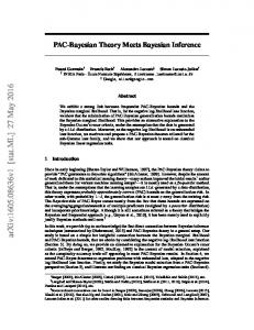
Thus, the final posterior-probability distribution is the same as the one we would have obtained in a single Bayesian analysis of both data sets combined. Note how the final posterior in the combined analysis is obtained by multiplying the likelihood functions f (XA⏐θ ) and f (XB⏐θ ) with the prior after appropriate normalization. Now, consider how knowledge about topology is accumulated in the framework of Bayesian phylogenetic inference (Figure 1). Before the analysis is started, a prior-probability distribution on trees is formulated. In the absence of background knowledge, all possible trees are given the same prior probability typically, a so-called uniform prior (Figure 1a). In most cases, different trees have very different probabilities of generating the observed data. These probabilities, or likelihoods, are simply multiplied with the corresponding prior probabilities to obtain the posterior probability of each tree. If the probabilities are measured on the log scale, we simply add the prior and likelihood scores to obtain the posterior score (Figure 1b). This is not a true probability distribution, however, because the probabilities do not sum to 1. After rescaling the values so that they do sum to 1, this is our posterior-probability distribution on trees (Figure 1c). Note that the normalization affects just the position of the baseline when probabilities are measured on the log scale; it leaves the relative tree probabilities (i.e., the absolute difference between log probabilities) unaffected. This is because normalization involves multiplication by a scaling factor, which is equivalent to addition of a constant value on the log scale. Now, if this posterior (Figure 1c) is used as the prior in a subsequent analysis, we need to add only the log-likelihood scores of the trees under the new data on top of the previous (unnormalized or normalized) posterior scores (Figure 1d). Renormalization results in the final posterior-probability distribution (Figure 1e). This distribution is equivalent to the posterior that would have been obtained in simultaneous Bayesian analysis of the two data sets combined (Figure 1f). The above description is somewhat simplified because topology does not specify a stochastic phylogenetic model fully. Typically, the parameter vector θ of such a model also includes branch lengths and substitution model parameters. We will return to this complication towards the end of the chapter; for now, we will ignore the other parameters and assume that θ contains only the topology (i.e., θ = τ).

Bayesian supertrees 1 2 3 4 5 6 7 8 9 10 11 12 13 14 15

1 2 3 4 5 6 7 8 9 10 11 12 13 14 15

0

0

-10

-10

-20

-20

(a)

(b)

-30

-30

log (probability)

1 2 3 4 5 6 7 8 9 10 11 12 13 14 15

1 2 3 4 5 6 7 8 9 10 11 12 13 14 15

0

0

-10

-10

-20

5

-20

(c) 1 2 3 4 5 6 7 8 9 10 11 12 13 14 15

(d) 1 2 3 4 5 6 7 8 9 10 11 12 13 14 15

10

10

0

0

-10

-10

(e)

(f) topology

Figure 1. Accumulation of evidence in Bayesian phylogenetic inference. All probabilities are given on a log scale and, because all are 1 specifying how much more probable a tree with the partition is compared with a tree without it (Huelsenbeck et al., 2002). For reasons that will become obvious later on, we refer to this as the Weighted Independent Binary (WIB) representation method. A single WIB factor r divides tree space into two classes of trees: those with the corresponding taxon bipartition b and those without it. A tree in the first class is r times more probable than a tree in the second class. If, as we will assume, the initial prior puts equal probability on all trees, then this statement is true for both the relative posterior probabilities f (τ⏐X ) and the relative likelihood scores f (X⏐τ ) of the trees. To calculate a factor r from the corresponding bipartition frequency s, assuming that the latter is the only factor changing the prior-probability distribution on trees, we need only know the number of trees in each class: ⏐T (bi+)⏐ and ⏐T (bi–)⏐. We have

(6)

and hence

() ()

r T bi+ s = 1− s T bi−

8

Ronquist et al.

r=

(7)

() s . T (b ) (1− s ) T bi−

+ i

The number of fully bifurcating trees supporting and opposing the taxon bipartition can be calculated easily. Suppose that B(n) is the number of fully bifurcating, unrooted trees for n taxa, and suppose that the bipartition b divides the n taxa into two sets with n0 and n1 taxa, respectively. The ratio of the number of trees with and without the partition is given by

(8)

( ) = B(n +1)B(n +1) , T (b ) B(n)− B(n +1)B(n +1)

T bi+

0

− i

1

0

1

where, from Felsenstein (1978),

(2n − 5)! ( ) n − 3 !2 = ∏ (2i − 5). ( ) n

(9)

Bn =

n−3

i=3

The formula in equation (8) follows from two facts: 1) the number of possible subtrees one can form on one side of the partition is equivalent to the number of rooted trees for the taxa on that side of the partition, and 2) the number of rooted trees for n taxa is equivalent to the number of unrooted trees for n + 1 taxa (Felsenstein, 1978). When we introduce more than one partition factor, the situation becomes more complicated. With k compatible partitions and partition-associated factors, we will be dividing tree space into 2k classes, each class containing trees with a unique combination of partition factors. For instance, assume that we have five taxa and score the frequency of two compatible bipartitions b1 and b2, which are also the most supported bipartitions. The corresponding factors r1 and r2 divide the 15 possible unrooted trees for five taxa into four classes (Table 1). One tree is compatible with both partitions and has the predicted relative probability r1r2. Two trees are compatible with partition 1 but not partition 2, and have predicted relative probability r1, whereas two other trees have predicted relative probability r2, and are compatible with partition 2 but not with partition 1. Finally, ten trees are not compatible with either partition and have predicted relative probability 1. Because each partition frequency is affected by both factors, we cannot obtain the partition factors independently from the corresponding partition frequencies. Instead, we need to solve the equation system

Bayesian supertrees

9

Table 1. WIB representation of a five-taxon tree space using two multiplicative factors r1 and r2 associated with compatible taxon bipartitions. Compatible with partition 1 partition 2 yes yes yes no no yes no no

Number of trees 1 2 2 10

Predicted relative probability r1r2 r1 r2 1

( ) ( )

( (

) )

( ) ( )

( ) ( )

(10)

T b1+ , b2+ r1r2 + T b1+ , b2− r1 s1 = 1− s1 T b1− , b2+ r2 + T b1− , b2−

(11)

T b1+ ,b2+ r1r2 + T b1− ,b2+ r2 s2 = . 1− s2 T b1+ ,b2− r1 + T b1− ,b2−

Some extra notation will help us generalize this equation system. Suppose that c is a matrix with each row ci defining a set of fully bifurcating trees by a vector of zeros and ones and recording whether the trees should be consistent with (1) or inconsistent with (0) the corresponding bipartition. That is, if cij = 1, then the trees in the set ci are consistent with partition bj; if cij = 0, then the trees in the set ci are inconsistent with partition bj. Furthermore, let N (ci) be the number of fully bifurcating trees consistent with the specified constraints. Now, obtaining the k partition factors involves solving the equation system

(12)

s1 1− s1

⎛ ⎜ N ci i, ci1 =1⎝ ⎛ ⎜ N ci i, ci1 =0 ⎝

( )∏ r ( )∏ r

∑ = ∑

⎞ ⎟ ⎠ cij ⎞ j ⎟ ⎠

cij j

j

j

M

(13)

sk = 1− s k

⎛ ⎜ N ci i, cik =1⎝ ⎛ ⎜ N ci i, cik =0 ⎝

∑ ∑

( )∏ r ( )∏ r j

j

⎞ ⎟ ⎠ . cij ⎞ ⎟ j ⎠

cij j

10

Ronquist et al.

The above equation system can be solved numerically using NewtonRaphson’s method or the secant method. Table 2 provides some examples of WIB factors calculated for a six-taxon tree to give a feel for the interaction between bipartition factors. Note that the factor associated with a particular support value varies greatly depending on context. If surrounding parts of the tree are well supported, the factor is smaller than if the surrounding parts are poorly supported. Even if all bipartitions have the same support, the factor will vary depending on whether it is associated with a peripheral or a central branch in the tree. The factor will be higher for a central branch simply because the proportion of trees consistent with the partition is smaller. Thus, it takes a stronger data factor to tip the result in favor of trees with such a bipartition. Some results are clearly counterintuitive. For instance, a bipartition frequency of 0.95 is associated with a stronger data effect if the other two partitions have frequencies of 0.70 and 0.95 than if both the other partitions have frequencies of 0.70.

5.

A parsimonious excursion

Assume that we find an optimal or near-optimal, fully bifurcating reference tree. In the Bayesian context, the reference tree can be the tree with maximum posterior probability (the MAP tree), or it can be obtained by building a fully resolved tree starting with the most frequent bipartition in the MCMC tree sample and then adding compatible bipartitions in order of decreasing frequency, a heuristic procedure that is likely to produce a good estimate of the MAP tree. The WIB factors are calculated from the frequencies of the bipartitions in the reference tree. Now we can understand the WIB method as classifying trees into different groups according to their distance from the reference tree using a single-sided, weighted partition metric (Robinson and Foulds, 1981), in which the weights are the WIB factors on the reference tree rather than on the edge lengths on both trees as Robinson and Foulds suggested originally. Like all partition metrics, WIB representation divides the part of tree space that is close to the reference tree very finely, whereas it loses its resolving power quickly as one moves away from the reference tree. Once all bipartitions in the reference tree have been lost, the WIB representation

Bayesian supertrees

11

Table 2. Hypothetical examples of partition frequencies (s) and partition factors (r) for an asymmetric six-taxon tree (as in Figure 4a). For each example, the value listed in the middle is the central branch in the tree (i.e., number 2 in Figure 4a). The partition odds (o) are calculated using the formula o = s / (1 – s). The partition factors (r) are given for both the WIB and the WAB methods, and were calculated by solving the appropriate equation system numerically. Finally, upper and lower bounds on the partition factors are given according to formulas discussed in the text. For the upper-bound equation, n is the number of trees without the partition divided by the number of trees with the partition. s1–s3

o

0.70 0.70 0.70 0.80 0.80 0.80 0.90 0.90 0.90 0.95 0.95 0.95 0.80 0.70 0.80 0.90 0.70 0.90 0.95 0.70 0.95 0.80 0.70 0.70 0.90 0.70 0.70 0.95 0.70 0.70

2.33 2.33 2.33 4.00 4.00 4.00 9.00 9.00 9.00 19.0 19.0 19.0 4.00 2.33 4.00 9.00 2.33 9.00 19.0 2.33 19.0 4.00 2.33 2.33 9.00 2.33 2.33 19.0 2.33 2.33

WIB r 6.79 9.11 6.79 10.43 12.95 10.43 20.74 23.48 20.74 40.89 43.75 40.89 11.76 7.21 11.76 26.44 5.76 26.44 55.56 5.18 55.56 12.03 8.08 6.65 27.99 7.15 6.50 60.11 6.73 6.42

WAB ln (r) 1.92 2.21 1.92 2.34 2.56 2.34 3.03 3.16 3.03 3.71 3.78 3.71 2.46 1.98 2.46 3.27 1.75 3.27 4.02 1.64 4.02 2.49 2.09 1.90 3.33 1.97 1.87 4.10 1.91 1.86

r 6.06 8.32 6.06 9.71 12.20 9.71 20.17 22.90 20.17 40.51 43.37 40.51 10.75 6.95 10.75 25.10 5.72 25.10 54.04 5.17 54.04 10.58 7.62 6.15 24.25 6.96 6.25 51.71 6.65 6.30

ln (r) 1.80 2.12 1.80 2.27 2.50 2.27 3.00 3.13 3.00 3.70 3.77 3.70 2.37 1.94 2.37 3.22 1.74 3.22 3.99 1.64 3.99 2.36 2.03 1.82 3.19 1.94 1.83 3.95 1.89 1.84

Min. ln (2o) 1.54 1.54 1.54 2.08 2.08 2.08 2.89 2.89 2.89 3.64 3.64 3.64 2.08 1.54 2.08 2.89 1.54 2.89 3.64 1.54 3.64 2.08 1.54 1.54 2.89 1.54 1.54 3.64 1.54 1.54

Max. ln (no) 2.64 3.21 2.64 3.18 3.75 3.18 3.99 4.56 3.99 4.74 5.31 4.74 3.18 3.21 3.18 3.99 3.21 3.99 4.74 3.21 4.74 3.18 3.21 2.64 3.99 3.21 2.64 4.74 3.21 2.64

no longer distinguishes between trees regardless of the fact that they often differ widely both in their resemblance to the reference tree and in their

12

Ronquist et al.

# tree classes (log scale)

108 107

ABa

106

ABs 3k

105 104 103

2k = IB

102 101

4

8

12

16

20

# taxa

Figure 2. Number of unique tree classes in IB and AB representation. With the IB method, trees are divided into 2k classes, where k is the number of interior branches in the reference tree. By contrast, the number of AB classes grows almost as fast as 3k for large trees. The number of unique tree classes is somewhat smaller for symmetric trees (ABs) than for asymmetric (comb-shaped) trees (ABa). Because the number of tree classes is given on a log scale, the difference in number of classes between AB and IB representation is dramatic for trees of any decent size.

actual posterior probability. This unresolved portion of tree space becomes more and more dominant as the number of taxa increases. Work on supertree construction using parsimony analysis suggests that there is an alternative factorial representation that extends the resolved part of tree space further away from the reference tree. Much of this work emanates from two papers discussing how phylogenies can be converted into matrices of binary characters for parsimony analysis (Baum, 1992; Ragan, 1992). Both papers arrive at the same method: the reference tree is represented by one binary (two-state) character for each taxon bipartition specified by the tree. This is equivalent to the additive binary coding scheme (Farris et al., 1970) used, among other things, to represent trees in coevolutionary and biogeographic studies (Brooks, 1981), so let us call it the Additive Binary (AB) representation. AB representation is the method commonly referred to as MRP. The AB matrix has several interesting properties. One of them is that it effectively defines a distance metric on trees based on their parsimony scores. The more distant a tree is to the reference tree, the higher its score will be using the AB matrix. For small tree spaces, the AB representation is equivalent to the unweighted version of the WIB method, which we refer to as Independent Binary (IB) representation. The reason is that a binary character can only have the parsimony length of 1 or 2 on trees with five or fewer taxa, and this is equivalent to the presence / absence of the partition under IB representation. For larger tree spaces, however, AB divides the trees more finely than IB using the same number of factors (Figure 2). This is easy to understand in the parsimony framework. Assume that we start with

Bayesian supertrees

13

a matrix of binary characters, each representing one of the taxon bipartitions in the reference tree. In other words, each character is equivalent to one of the b vectors discussed previously. Now, the score of a tree under the AB representation is equivalent to the difference in parsimony length between that tree and the reference tree, plus the length of the reference tree. In the IB representation, however, the score is equivalent to the number of homoplastic characters plus the length of the reference tree. Essentially, the IB factors have an on-off effect, whereas the AB factors show a graded response, the range of which is determined by the way in which the binary character divides the taxa. If the binary character divides the taxon set into subsets with n0 and n1 taxa each, then the number of levels of the corresponding AB factor will be min(n0, n1). Not all combinations of AB factor levels are possible, but the AB factors nevertheless divide tree space into many more unique classes than the IB factors (Figure 2). For instance, a 20-taxon tree space will be divided into 130 000 classes by the IB method, but, depending on tree shape, into 3.1 to 6.5 million classes by the AB method. An obvious improvement of the AB representation is to take the relative support of different taxon bipartitions into account. In such a Weighted Additive Binary (WAB) representation, trees that differ from the best tree only in weakly supported parts will be scored as being better than those that do not retain strongly supported groupings. In parsimony analysis, support is commonly measured using either resampling techniques — the bootstrap or the jackknife — or the decay index (Bremer support, branch support). Any of these support measures can be used to calculate the weights of a WAB matrix. For instance, let us examine the bootstrap-weighting scheme (Ronquist, 1996). Assume that an AB character bi, which represents the partition i in the best tree, is assigned the weight ri. Furthermore, assume that the probability of drawing character bi in bootstrap resampling is ri / R, where R = ∑ ri, and that we count taxon bipartition i as being present in the bootstrap tree when at least one character of type bi is present in the resampled matrix. Then, the bootstrap support si for partition i would be given by the formula si = 1 – (1 – ri / R)R. If R is large, then (1 – ri / R)R ≈ e-ri and we can calculate the weight of a particular bipartition from its support value as ri = ln (1 / (1 – si)). If R is small, then ri can be calculated without using this approximation; for instance, by an iterative method where the initial ri and R values are obtained using the e-ri approximation, and then the exact formula is applied repeatedly until the R and ri values stabilize. When the resultant WAB matrix is subjected to bootstrap resampling, the bootstrap support values of the original analysis should be reproduced accurately.

14

Ronquist et al.

A more direct relation to the original parsimony scores is obtained in decay-index-derived WAB representation. The decay index di for a bipartition i is the difference in parsimony score between the best tree with the partition and the best tree without the partition. The di values can be used directly as the weights of the corresponding characters in the WAB matrix. The decay-index-derived WAB scores should be correlated highly with the original parsimony scores, and one might expect the regression coefficient to be close to 1 because the difference between two trees in WAB scores should reflect the difference between them in parsimony scores. Despite the difference in approach, we might also expect a close correlation between the bootstrap-derived WAB score of a tree and its parsimony length, although the expected value of the regression coefficient is unclear. To illustrate these different representation methods in the parsimony context, we used a data set of 54 drosophilid sequences of the nuclear protein-coding gene ADH (771 bp; Russo et al., 1995). A set of 1000 bootstrap replications was generated in PAUP* v4.0b10 (Swofford, 2002), each analysis using one simple stepwise addition sequence, with Drosophila persimilis as the reference taxon, followed by TBR swapping. A fully resolved reference tree was assembled from the bootstrap bipartition frequencies by adding compatible bipartitions in order of decreasing frequency until the tree was fully resolved (only three bipartitions had frequencies less than 0.50). Bootstrap weights of bipartition factors were calculated as ln(1 / (1 – (1000s / 1001))), as if there had been one extra replication without all bipartitions. Without this correction, it is impossible to calculate the weights of the best supported bipartitions with s = 1.0 because ln(1 / 1 – s) = ln(1 / (1 – 1)) = ln(1/0) is undefined. The correction gives a minimum estimate of the strength of the factor associated with these partitions. The decay indices associated with the bipartitions of the reference tree were calculated in a series of constrained searches in PAUP* using the same heuristic strategy as the bootstrap searches. Finally, we generated 1000 random trees and compared their score using the original data with their score using unweighted, decay-index-weighted, and bootstrap-weighted versions of the IB and AB methods (Figure 3). Because the random trees were distant from the reference tree, the IB and WIB representations failed miserably in predicting tree scores (Figures 3a, c, e). However, all AB and WAB representations provided surprisingly good pictures of tree space, with the weighted versions providing a slight improvement over the unweighted one (Figures 3b,d,f). It is somewhat surprising that weighting does not improve the AB-based prediction more; however, as one moves closer to the reference tree, the importance of weighting the factors should increase. This is indicated by the results for smaller datasets reported by Ronquist (1996), in which random trees were

Bayesian supertrees

15

330

102

310 101

290

270 100

(a)

predicted tree score

4100

(b)

4300

4500

4700

4900

5100

250 4100

4300

4500

4700

4900

5100

4300

4500

4700

4900

5100

4300

4500

4700

4900

5100

1900

650 640

1800

630

1700

620 1600

(c)

610 4100

4300

4500

4700

4900

5100

(d)

4100

780 287 740

283

700

279

(e)

275 4100

(f)

4300

4500

4700

4900

5100

660 4100

actual tree score

Figure 3. Performance of different representation methods in predicting the parsimony scores of 1000 random trees for a 54-taxon data set of drosophilid ADH sequences: a) IB representation, b) AB representation, c) decay-index-weighted WIB representation, d) decay-index-weighted WAB representation, e) bootstrap-weighted WIB representation, and f) bootstrap-weighted WAB representation.

closer to the reference tree (Table 3). The IB and WIB methods were not included in this study, but one would expect the WIB representation to outperform IB as well as AB representation (equivalent to MRP) in the region close to the reference tree because the latter representation will be similar to IB in this part of tree space. Thus, given the success of the WAB method in the parsimony context, is it possible to use it for describing Bayesian tree probabilities?

16

Ronquist et al.

Table 3. Performance of AB, decay-index-weighted WAB, and bootstrap-weighted WAB representation in predicting parsimony tree scores of 1000 random trees for some different morphological data sets (modified from Ronquist, 1996). Data set

Taxa

Characters

Liopteridae Cynipidae 2 Ibaliidae Cynipoidea Cynipidae 2

11 12 18 19 32

54 108 82 110 158

6.

Coefficient of determination (r2) WABb AB WABd 0.833 0.933 0.929 0.889 – 0.852 0.686 0.922 0.912 0.867 0.933 0.929 0.642 – –

Weighted additive binary representation

Implementing WAB representation in the Bayesian framework is actually straightforward: we just translate each parsimony step in a WAB factor to a constant difference in log-likelihood scores between trees. For instance, assume that the binary parsimony character associated with a WAB factor r can have one, two, or three steps on different trees. The trees with two steps are then r times as likely as those with three steps. Similarly, the trees with one step are r times more likely than those with two steps and r2 times more likely than those with three steps. To solve for WAB instead of WIB factors, we make the following changes to our previous notation. Assume that l (bi, ci) is the parsimony length of the binary character bi on trees in the set defined by ci and that g (bi) is the maximum parsimony length of character bi on any tree. Now, let c be the matrix containing all unique rows ci, where each element cij ∈ (0, …, g (bj)). Each row ci will then define a set of trees where l (bj,ci) = g (bi) – cij. In some cases, the set will be empty; these rows can be deleted from c for more efficient calculation. With these changes, we can solve for the WABpartition factors using the same equation system defined above for the WIB factors (equations (12) to (13)). The only difference is that we must account for the fact that the elements of c might be greater than 1. The equation system thus becomes

(14)

s1 1− s1

⎛ ⎜ N ci i, ci1 ≥1⎝ ⎛ ⎜ N ci i, ci1 =0 ⎝

( )∏ r ( )∏ r

∑ = ∑

M

j

j

⎞ ⎟ ⎠ cij ⎞ j ⎟ ⎠

cij j

Bayesian supertrees D. picticornis D. affinidisjuncta D. planitibia D. adiastola D. nigra D. mimica

1

(a) 2

3

D. ambigua D. melanogaster D. sechellia Z. tuberculatus D. mimica D. borealis D. virilis_2 D. mettleri D. buzzatii_1 D. mojavensis_2

1

2 3

(b)

6 4 5

17

7

Figure 4. Subsets of the drosophilid data set used to examine factorial representation of Bayesian tree probabilities: (a) a six-taxon subset representing a small subsection of the best tree for the full data set, and (b) a ten-taxon subset spanning the entire best tree for the full data set. The taxon bipartition numbers are the same as those in Table 4.

(15)

sk = 1− s k

∑ ∑

⎛ ⎜ N ci

( )∏ r ⎛ ⎜ N (c )∏ r ⎝

i, cik ≥1⎝

i, cik =0

i

j

j

⎞ ⎟ ⎠ . cij ⎞ ⎟ j ⎠

cij j

Note that there will be more rows in the c matrix when we solve for WAB factors, reflecting the larger number of tree classes, but the number of WAB factors is still k. Asymmetric six-taxon trees are the smallest reference trees for which WIB- and WAB-representation methods differ: WIB representation results in eight tree classes, whereas WAB representation results in nine. Examination of hypothetical support values for such trees (Table 2) reveals that WIB and WAB factors are generally similar, although not identical. When they differ, WAB factors are smaller than WIB factors. As the support level increases, the WIB and WAB factors become more similar. To illustrate the efficiency of WIB and WAB representation in describing empirical Bayesian tree probabilities, we selected a six-taxon and a ten-taxon subset of the 54-taxon drosophilid ADH data set (Figure 4). For each data set, the best (MAP) tree was estimated through MCMC sampling (1 000 000 generations, sampled every 100th generation, first 50% of samples discarded as burn-in) under the GTR model with site-specific rates using MrBayes 3.0b4 (Ronquist and Huelsenbeck, 2003). Default values in MrBayes 3.0b4 were used for priors and other settings. For both data sets, all taxon bipartitions in the MAP tree were strongly supported.

18

Ronquist et al.

For the six-taxon data set, there are 105 possible unrooted trees, which the WIB and WAB methods divide into eight and nine classes, respectively, based on the reference tree. For the ten-taxon data set, there are about 2 × 106 different trees, which are divided into 128 (WIB) or 290 (WAB) classes based on the reference tree. For the six-taxon tree, we estimated the marginal posterior probability of each of the 105 possible trees using the harmonic mean of the likelihood values (Newton et al., 1994; for a discussion of alternative estimators of marginal likelihood values, see Gamerman, 1997) by feeding the program with the appropriate starting tree and setting the proposal probability of all topology proposals to zero. The estimated tree probabilities were used, in turn, to estimate the odds oi = si / (1 – si) for each taxon bipartition. For the ten-taxon problem, we used a similar approach, except that we selected one tree randomly from each of the 290 WAB classes and used only 500 000 generations in each topologyconstrained MCMC analysis. To increase the accuracy of the estimates of bipartition odds, we also estimated the marginal posterior probabilities for all trees differing from the reference tree with a WAB score of two or less, and included them in the estimate together with the 290 random trees, deleting duplicates. The bipartition odds were used to obtain the corresponding WIB and WAB factors by solving the appropriate equation system (i.e., (12) to (13)) using the secant method (Table 4). Finally, the estimated posterior tree probabilities were plotted against the tree probabilities predicted by the WIB and WAB methods (Figure 5).

Bayesian supertrees

19

Table 4. Measures of support for the six-and ten-taxon examples (Figures 4 and 5). The partition odds (o) were estimated from marginal tree probabilities as described in the text, and the partition factors (r) were calculated from these by solving the appropriate equation system. For these well-supported example trees, the WIB and WAB factors (r) are identical to the precision reported here. As predicted, the factors are higher than the corresponding partition odds. Two methods of estimating the factors are given. One is based on taking twice the partition odds (2o), which provides a lower bound on the factors. The other method is based on the harmonic mean (h) of the estimates from the two near-optimal trees breaking only that partition. Both methods provide accurate approximations of the partition factors. Partition Six-taxon tree 1 2 3 Ten-taxon tree 1 2 3 4 5 6 7

ln (o)

ln (r)

ln (2o)

ln (h)

4.76 6.89 4.08

5.45 7.62 4.78

5.45 7.58 4.78

5.45 7.56 4.77

32.77 73.89 31.82 5.85 9.25 45.60 4.65

33.46 74.58 32.52 6.54 9.96 46.30 5.34

33.46 74.58 32.51 6.54 9.94 46.29 5.34

33.75 75.81 32.51 6.65 9.94 46.32 5.38

For the six-taxon tree space, the WIB and WAB methods were very similar (Figures 5a, b). The WAB method split the worst trees into two classes, making the predicted probabilities match the actual probabilities better. The best trees had a probability that matched the predicted value closely (line in diagram). For the poor trees, the maximum probability of trees in each class was predicted more accurately than the average probability. For the ten-taxon trees, we saw much more of a difference between WIB and WAB representations (Figures 5c, d). Both methods predicted the nearoptimal trees accurately and overestimated the probability of poor trees. However, the WIB prediction degraded quickly as we moved away from the reference tree, whereas the WAB prediction remained distinctly correlated with the actual tree probability all the way to the trees that were most distant from the reference tree. Given that there are about two million trees in this tree space, it is remarkable that the WAB method managed to capture so much of its properties with only seven weighted factors. Is the increased power of the WAB method important in the Bayesian context? There are several reasons to suggest that the answer is yes. First, if there is significant conflict between the data set at hand and a prior based on

20

Ronquist et al. (a)

-ln (predicted tree probability)

25

(b)

25

20

20

15

15

10

10

5

5

0

0 0

400

10

20

30

40

0

50

400

(c)

300

300

200

200

100

100

0

10

20

30

40

50

(d)

0 0

200

400

600

800

0

200

400

600

800

-ln (actual tree probability)

Figure 5. Factorial representation of Bayesian tree spaces for a six- and a ten-taxon (Figures 4a, b, respectively) example: a) WIB representation of the six-taxon tree space, b) WAB representation of the six-taxon tree space, c) WIB representation of the tentaxon tree space, and d) WAB representation of the ten-taxon tree space. The line marks perfect prediction of tree probabilities. All tree probabilities are measured relative to the best tree.

the results from a previous analysis, then it becomes important to know what the previous analysis implied concerning the relative probabilities of trees that were poor in that analysis. Second, as trees become larger, the portion of tree space resolved by the WIB method becomes smaller. For large trees, the portion of tree space resolved by the WIB method might be simply too small for an appropriate description of the probability distribution on trees. Third, an MCMC sampler needs to move across topology space to find all the trees it should sample from. The presence / absence nature of the WIB factors might cause artificial threshold effects that prevent an MCMC sampler from moving around in tree space as it should.

7.

Estimating bipartition factors

Solving the equation system (12) to (13), even with iterative numerical methods, is feasible only for relatively small trees. Thus, it is desirable to develop more computationally efficient ways of estimating the WIB and WAB partition factors.

Bayesian supertrees

7.1

21

Upper and lower bounds

One can find upper and lower bounds on the WIB factors quickly and easily by focusing on the bipartition-odds equation,

r1 =

(16)

()s , T (b )1− s T b1−

1

+ 1

1

which is valid when there is only one factor affecting tree probabilities. The equation says that the partition factor r1 equals the ratio of inconsistent to consistent trees times the partition odds (ratio of samples with and without the partition). The fewer the consistent trees are in number relative to the inconsistent trees, the stronger the partition factor must be to achieve the observed partition frequency. As we have seen, the ratio of inconsistent to consistent trees is determined by the number of taxa in the two partitions according to equations (8) and (9). If we add a second taxon bipartition that is compatible with the first partition with the associated factor r2 > 1, we can use a similar equation for r1, but we need to take the altered probability of the other trees into account. Then we have

(17)

r1 =

( ) ( )s . T (b , b )r + T (b , b )1− s T b1− , b2+ r2 + T b1− , b2− + 1

+ 2

2

− 2

+ 1

1

1

How the addition of r2 affects the value of r1 depends on the relation between the ratio of the numbers we multiply with r2 (⏐T (b1– , b2+)⏐ / ⏐T (b1+, b2+)⏐) and the original ratio (⏐T (b1–)⏐ / ⏐T (b1+)⏐) (see equation (16)). If the ratio of numbers multiplied by r2 is smaller than the original ratio, the value of r1 will decrease. Because

(18)

( ) < T (b ), T (b , b ) T (b ) T b1− , b2+

− 1

+ 1

+ 1

+ 2

which can be shown using equations (8) and (9) to specify the number of trees satisfying each of the constraints, then r1 will always decrease when r2 is added. A similar argument can be used to show that r1 decreases when the next congruent partition is added, and so on. Therefore, the estimate of r1

22

Ronquist et al.

decreases monotonously as more and more compatible partitions are added to the equation, and, hence, equation (16) provides an upper bound on a WIB factor; that is,

(19)

ri ≤

()s . T (b )1− s T bi−

+ i

i

i

A lower bound on WIB factors is obtained by considering the case when all other possible taxon bipartitions are supported so strongly that we can ignore the trees inconsistent with them. Then we need to consider only the three remaining alternative trees centered on the taxon bipartition in focus, one of which is consistent with the bipartition and two of which are not. In other words, the lower bound on a WIB factor is (20)

ri ≥

2s i . 1− s1

Under similar conditions (all partitions are compatible), the lower and upper bounds of WIB factors apply to WAB factors as well. Actually, unlike WIB factors, it appears possible to derive a lower upper bound on WAB factors, but this is not attempted here. In practice, the real WIB or WAB factors are likely to be much closer to the lower than the upper bound, particularly in well-supported trees. This occurs because the upper bound is associated with trees in which all nodes except the one being examined have frequencies close to zero (given that the tree is not extremely small). Even a weakly supported tree is unlikely to be close to this situation. Thus, the lower-bound equation can be used as a good-and-fast approximation of the real partition factors. For example, for the well-supported six- and ten-taxon trees examined above, the lower-bound equation provides a very accurate approximation of the partition factors (Table 4). In trees with less strongly supported partitions, the partition factors will be considerably higher than the lower bound, but still far removed from the upper bound (Table 2).

7.2

Estimating partition odds directly

A problem with the lower-bound approximation is that the partition odds on which it is based are difficult to estimate for well-supported partitions. When a partition frequency approaches 1.0, the ordinary estimate of the odds (i.e., the ratio of samples with and without the partition) becomes unstable because there will be few MCMC samples without the partition. Indeed, one

Bayesian supertrees

23

encounters frequently partitions that are present in all MCMC samples, in which case this estimate becomes undefined (division by zero). A possible approach then is to estimate the odds using n / 1, where n is the number of MCMC samples, as if one had observed one sample without the partition. This solution is analogous to the one used above in calculating bootstrapderived weights for WAB or WIB characters. An obvious disadvantage of this method is that it puts an artificial cap on the values of partition factors, which will distort the factorial representation of tree probabilities unnecessarily. Furthermore, the method does not address the difficulty of estimating partition odds accurately when there are only few sampled trees conflicting with the partition. For instance, one or two sampled trees without the partition translates to a difference in estimated odds by a factor of two, which becomes important when one realizes that stochastic effects might well result in some runs giving one without the partition, whereas others will give two. A better (although computationally more complex) approach to estimating extreme partition odds is to evaluate the marginal likelihood of the alternative hypotheses using separate MCMC analyses, one constrained to sample from trees with the partition and the other one constrained to sample from trees without it. There are several estimators of the marginal likelihood that can be used for this purpose, of which the harmonic mean of the likelihood values used above (Newton et al., 1994) is the easiest one to implement. In our experience, this estimator is stable enough to provide a rough approximation of the likelihood ratio of the contrasting hypotheses. A more accurate estimate can be obtained in a subsequent analysis by increasing the likelihood of the trees inconsistent with the examined bipartition artificially such that the two alternative hypotheses can be contrasted in a single MCMC run.

7.3

Estimating partition factors directly

Similar methods can be used to estimate partition factors directly without calculating the partition odds first. Any pair of trees that differ from each other solely by a single step in one WAB factor could be used in estimating the magnitude of that factor because the factor is a predictor of the likelihood ratio of the trees. One way of utilizing this fact would be to estimate the partition factors in the reference tree by a series of searches, in each of which all bipartitions of the reference tree are fixed except one. This would leave only three alternative topologies (one consistent and two inconsistent with the bipartition) to be considered in estimating each partition factor. If the partition factor is weak, the relative probability of the three competing trees can be evaluated in a single run; if it is strong, one might have to estimate

24

Ronquist et al.

the likelihood scores of the two topologies that conflict with the partition in separate MCMC analyses or inflate their probability artificially to make accurate estimation of the factor possible in a single analysis, as discussed above for the estimation of partition odds. Because the topology space is so small for these analyses, they should be much less demanding computationally than those required in estimating partition odds. Our empirical results suggest that the harmonic mean of the estimates based on the two inconsistent trees comes very close to the true partition factor (Table 4). The method could be refined by examining two or more adjacent partitions at a time. The estimate of each partition factor would then be based on comparisons among more trees than the three used in the original formulation, but the computational burden would, of course, increase correspondingly.

8.

Partition factors: a better support measure?

The method of estimating partition factors suggests a similarity between partition factors and the probabilistic analog of the decay index. In the Bayesian context, the decay index would be the ratio between the marginal probabilities of the best trees with and without the partition. In many cases, the first tree would be the same as the reference tree and the second would differ only in that it was incongruent with the partition in question. Thus, the Bayesian decay index would be the same in many cases as selecting the minimum, rather than calculating the harmonic mean, of the two estimates of the partition factor based on near-optimal trees. To the extent that they differ, however, the partition factors should describe the partition-associated data effects more accurately than the decay indices, which will underestimate the effects systematically. In a sense, the partition factors provide the ultimate support measure, which are related to partition-associated data effects more intimately than both the decay index and the bipartition frequencies. The correlation between bipartition frequencies, in particular, and data effects is imprecise. A frequency of, say, 0.7 indicates considerable data support if it is associated with a partition in the middle of a poorly supported tree, but it implies only modest data support when tied to a peripheral partition in a well-supported tree. These effects are illustrated by the previously discussed hypothetical examples for a six-taxon data set (Table 2). In these, a taxon-bipartition frequency of 0.7 can be associated with a partition factor ranging from 5.2 to 8.3 depending on the context. Similarly, a taxon-bipartition frequency of 0.95 can translate to a partition factor ranging from 40.5 to 54.0. Larger trees will display even

Bayesian supertrees

25

more variability in the partition factors associated with a given partition frequency. Because the partition factors hold the key to the distribution of tree probabilities, which plays such a central role in Bayesian phylogenetic inference and supertree construction, it would be desirable if future Bayesian analyses reported partition factors in addition to, or even instead of, partition frequencies.

9.

Using partition factors to build supertrees

Using the WAB partition factors from one analysis to define a priorprobability distribution on trees for a subsequent Bayesian MCMC analysis is straightforward. As the MCMC procedure of the second analysis moves around among possible trees, it needs to evaluate the prior-probability ratio between trees from the partition factors. This is done easily by evaluating the difference in the WAB parsimony score of the trees using parsimony algorithms. The binary data matrix used in this step is exactly the same as the matrix used in MRP, except that the characters are weighted differently. Once the prior ratio is obtained, the likelihood ratio of the trees is calculated using standard procedures and the MCMC analysis proceeds as usual. A possible complication that might occur is that the WAB representation introduces some artificial step effects in the distribution of prior tree probabilities, which might cause difficulties for the MCMC procedure. Only empirical studies can determine whether this is an issue in real analyses, and this is outside of the scope of the present chapter. However, we note that the improved resolution of WAB representation over WIB representation should help to alleviate this problem. Similar considerations suggest that Bayesian analyses constrained by a single partition factor should use WAB rather than WIB in translating the partition factor to prior tree probabilities. Building a composite prior from several previous analyses only involves combining several WAB matrices. If there is partial rather than complete taxon overlap among the previous analyses, the WAB characters are simply coded as missing observations for the taxa that are not represented in the reference tree of a particular analysis. This results in the position of the missing taxa having no effect on the tree probabilities from that analysis, as is appropriate. The previous analyses need not be Bayesian as long as the results can be interpreted in terms of probabilities. For instance, the bootstrap proportions from a parsimony analysis could be treated simply as if they were Bayesian clade probabilities. This should result in a reasonable prior, given that the parsimony criterion is consistent for the type of data analyzed. Even a tree presented without support values could be accepted as providing some prior evidence concerning topology. One possible way of

26

Ronquist et al.

converting such a tree into probabilities would be to assume that each clade (taxon bipartition) was supported by one character in a parsimony analysis, corresponding to a bootstrap proportion of roughly 0.63 (ln(1 / (1 – 0.63)) ≈ 1.0). The independence of previous analyses is an additional problem that should be considered (see also Gatesy and Springer, 2004). Clearly, it is inappropriate to multiply the probabilities together from two previous analyses if they are based on the same or very similar data. Expressing prior knowledge in terms of probabilities is difficult and it is important to describe the approach taken clearly and to examine the robustness of the conclusions to alternative ways of formulating the prior. As synthesis becomes increasingly important in phylogenetics, however, it is a challenge that has to be faced. Constructing a Bayesian supertree is the same thing as sampling from a composite prior assembled by combining WAB matrices without adding any new data. As long as the WAB matrices provide efficient descriptions of the Bayesian tree probabilities and the underlying analyses and models are independent (see below), the supertree space is fully specified statistically. Perhaps the most intriguing aspect is that the supertree space can be sampled by an MCMC procedure considerably faster and more intelligently than an ordinary tree space. Sampling from an ordinary tree space involves calculating the likelihood ratios of trees, a computationally expensive operation that is responsible for the bulk of the execution time of a Bayesian MCMC analysis. Sampling from a supertree space requires only evaluation of the difference between two trees in weighted parsimony scores, a vastly more efficient operation. Using published shortcuts (Goloboff, 1996; Ronquist, 1998), this can be completed in time dependent linearly on the number of WAB factors, but independent of supertree size. Even more intriguing, the supertree space can be sampled using fully conditional (Gibbs) sampling. In normal MCMC sampling of topologies (using the Metropolis algorithm), new trees are proposed according to a proposal distribution and then evaluated according to their posterior probability. Because of the difficulties of formulating a good proposal distribution, most proposed trees have low posterior probability and are rejected. This leads to computational inefficiency; it is not unusual to see 90% or more of topology proposals being rejected, making it necessary to run the MCMC procedure much longer than otherwise necessary. In Gibbs sampling, however, the proposal distribution is the same as the posterior-probability distribution conditional on the present state (Gelman et al., 1995). This results in automatic acceptance of all proposals and more efficient MCMC sampling. In the Bayesian supertree context, one could implement Gibbs sampling for topologies easily. For instance, one could propose a new tree by erasing a few adjacent nodes in the existing tree, then calculate the parsimony score

Bayesian supertrees

27

(log probabilities) of all possible ways of reconstructing a fully bifurcating tree, and finally select among these according to their relative probabilities. Given these considerations, it is clear that the construction of a Bayesian supertree is comparable in computational complexity to the construction of a supertree using parsimony analysis of weighted or unweighted MRP matrices. Indeed, there are reasons to expect the Bayesian MCMC approach to be more efficient than parsimony. First, sampling a tree space adequately can be easier than exploring large islands of optimal or near-optimal trees. Second, the random component of MCMC sampling often appears to provide an efficient way of climbing from trees with poor likelihood scores to trees with optimal or near-optimal scores without becoming trapped in local optima. These advantages come in addition to the fact that the Bayesian supertree space is based on fully specified evolutionary models, with all the benefits associated with such an approach.

10.

Model independence assumption

Now it is time to return finally to the assumption made at the beginning of this chapter, namely that we could focus entirely on the topology parameter and ignore the other parameters in the phylogenetic model. As stated then, the phylogenetic model typically includes branch length and substitution model parameters in addition to topology. When a diffuse or noninformative prior is formulated, each parameter is associated typically with a completely independent probability distribution. Thus, the joint probability of a particular topology and a particular set of branch lengths, for example, is calculated by simply multiplying the probability of the topology and the probability of the branch lengths. When the posterior is obtained, it is not solely a probability distribution on trees; it is a joint-probability distribution on all the parameters in the model. The posterior tree probabilities we have been discussing so far are marginal probabilities that are obtained by integrating and summing out other parameters in the phylogenetic model from the joint posterior-probability distribution. What happens when we embark on a subsequent analysis and want to use the posterior distribution from the first analysis as the prior in the next? If the non-topology parameters for the new data set are entirely independent from those of the old data set, we can use the marginal tree probabilities without any problems. This involves assuming that, for instance, the branch length parameters are independent among partitions. If, some of the nontopology parameters are shared, however, we should take this into account. Unfortunately, this is rather complicated because of the dependence among parameters. In particular, branch-length parameters are likely to be highly dependent on topology. For instance, the joint posterior-probability

28

Ronquist et al.

distribution from the first analysis might specify that the probability of a certain branch (corresponding to a certain taxon bipartition) being of length v is p1 on topology 1 and p2 on topology 2. Similarly, if the branch is of length v1, topology 1 might be p1 more probable than topology 2, whereas a length of v2 implies that topology 1 is p2 more probable than topology 2. There are at least two possible ways to address this dependence among parameters. One is to ignore that the non-topology parameters are shared across data sets, which will obviously result in some loss of information. If the only effect is to make the probability distribution on trees slightly more diffuse, however, this might be a cheap price to pay for the ability to build supertrees. Another simplifying approximation, which will work for some parameters but not for branch lengths, is to ignore the dependence and use the marginal posterior distributions as truly independent priors. For instance, the posterior-probability distributions of GTR rate parameters or stationarystate frequencies might often be sufficiently robust to changes in topology that the dependence between these distributions can be ignored safely. In conclusion, then, it is often justifiable to use the marginal posterior tree probabilities of one Bayesian analysis as an independent priorprobability distribution on trees in a subsequent analysis, ignoring model parameters shared across data sets.

11.

Synthesis

Supertree construction is viewed usually as a procedure that takes trees resulting from individual phylogenetic analyses and puts them together into a larger tree. The Bayesian approach, with its emphasis on probability distributions, does not fit easily into this scheme. The result of Bayesian phylogenetic inference is not a single tree, but a distribution of tree probabilities. To build a true Bayesian supertree, we need to combine probability distributions on trees, not single trees. As we have seen, tree probability distributions are difficult to handle because of the enormous size of tree space. To work with tree probability distributions, we need efficient ways of describing them and taxonbipartition frequencies have become the standard tool in Bayesian phylogenetic inference. The partition frequencies are statements about the relative probability of different classes of trees, but they do not allow direct calculation of individual tree probabilities. To accomplish that, we have described two ways of translating partition frequencies to approximate tree probabilities. Both rely on the assumption that there are independent partition-associated multiplicative data effects. In one method (WIB), each data effect is either present or absent depending on whether or not the taxon bipartition is represented in the tree. In the other (WAB), there is a graded

Bayesian supertrees

29

response depending on the extent to which the tree conflicts with the taxon bipartition represented by the data effect. The level of the effect is determined by the parsimony score of a binary (MRP) character describing the partition. We have seen that the latter approach is superior in describing the tree-probability distribution, particularly for that part of tree space far removed from the best trees. We have also seen that the WAB data factors can be calculated rapidly from partition frequencies using the lower-bound estimate or estimated more accurately using specifically designed Bayesian MCMC analyses. WAB matrices from individual Bayesian analyses can be used to specify a prior-probability distribution on subsequent analyses. By combining several WAB matrices, we can define a supertree space that has special properties that reduce the computational complexity of sampling from it with Bayesian MCMC methods. We think that the field of supertree construction in general would benefit from more of a Bayesian perspective on phylogenetic inference. Instead of viewing phylogenetic methods as producing a single tree, we should focus on the way they translate data sets to distributions of tree scores (parsimony scores, maximum likelihood scores, bootstrap proportions). Just picking a single tree from each analysis amounts to discarding most of the information in the data. MRP is often regarded as a way of coding a single tree for inclusion in a supertree, but it is also an excellent way of summarizing tree scores. The tree used to derive the MRP characters is just a vehicle for finding the significant partition-associated data effects. As shown here and elsewhere, MRP is a surprisingly efficient key to the entire distribution of tree scores in the original analysis, particularly if the MRP characters are weighted differentially (Ronquist, 1996; Bininda-Emonds and Sanderson, 2001). The success of bootstrap-derived and, in particular, decay-indexderived weights in improving MRP prediction of tree scores can be understood easily because of their similarity to WAB partition factors. Indeed, the Bayesian WAB perspective suggests new and efficient ways of calculating MRP weights. There has been much emphasis lately on the advantages of polynomialtime algorithms for constructing supertrees (e.g., Semple and Steel, 2000; Steel et al., 2000; Page, 2002, 2004). However, the polynomial-time algorithms (e.g., MINCUTSUPERTREE; Semple and Steel, 2000) that have been discussed so far in the supertree context are consensus-like techniques that typically take one tree from each analysis as input and, therefore, ignore the distribution of tree scores. They can be improved by inputting sets of weighted trees from each analysis, but even a large set of weighted trees is a far less efficient way of representing the distribution of tree scores than factorial methods such as WAB. Ultimately, the choice of supertree method must depend on a balance between speed and accuracy. Factorial methods

30

Ronquist et al.

have the upper hand when it comes to accuracy, and supertrees can be constructed undoubtedly from factorial supermatrices using standard polynomial-time tree construction algorithms. We suspect, however, that many systematists will prefer more powerful supertree inference techniques. What is the computational complexity of building fully Bayesian supertrees based on MCMC sampling from tree spaces defined by WAB supermatrices? As we have tried to show, there is nothing to suggest that these analyses would be more complex computationally than parsimony analyses. Given that the parsimony method has been applied successfully to problems with thousands of sequences, it should be possible to construct Bayesian supertrees of at least this size. By being based on fully specified evolutionary models, the Bayesian method potentially could make more efficient use of the underlying information than all alternative supertree methods available today. What developments are necessary to enable the construction of Bayesian supertrees on a grand scale? Not much. Reporting taxon-bipartition frequencies is common practice already in Bayesian phylogenetic inference, and the frequencies can be converted rapidly to partition factors using the approximation based on the lower-bound equation as described above. However, as discussed in detail in this chapter, it is possible to estimate the partition factors more accurately, and it would be advantageous if it became standard practice to report such partition-factor estimates in addition to the partition frequencies in Bayesian analyses. Constructing an MCMC algorithm that samples from a supertree space defined by a WAB supermatrix is straightforward. In the near future, we hopefully will see the first Bayesian supertrees reported and learn more about the potential of this approach to supertrees.

Acknowledgements We would like to thank Olaf Bininda-Emonds for inviting us to write this chapter and for being patient with its delivery. Lars Cederberg performed some of the analyses. Sverker Holmgren, Karljohan Lundin, and Lars Gustavsson provided invaluable help in developing numerical methods for calculating partition factors from taxon bipartition frequencies. Olaf Bininda-Emonds, Rutger Vos, and an anonymous reviewer provided comments that helped improve the original version of the chapter. FR was supported by the Swedish Research Council (grant 621–2001–2963) and JPH by the National Science Foundation (grants DEB–0075406 and MCB– 0075404).

Bayesian supertrees

31

References BAUM, B. R. 1992. Combining trees as a way of combining data sets for phylogenetic inference, and the desirability of combining gene trees. Taxon 41:1–10. BAUM, B. R. AND RAGAN, M. A. 2004. The MRP method. In O. R. P. Bininda-Emonds (ed). Phylogenetic Supertrees: Combining Information to Reveal the Tree of Life, pp. xxx–xxx. Kluwer Academic, Dordrecht, the Netherlands. BININDA-EMONDS, O. R. P. AND BRYANT, H. N. 1998. Properties of matrix representation with parsimony analyses. Systematic Biology 47:497–508. BININDA-EMONDS, O. R. P. AND SANDERSON, M. J. 2001. Assessment of the accuracy of matrix representation with parsimony analysis supertree construction. Systematic Biology 50:565– 579. BROOKS, D. R. 1981. Hennig’s parasitological method: a proposed solution. Systematic Zoology 30:229–249. FARRIS, J. S., KLUGE, A. G., AND ECKHARDT, M. J. 1970. A numerical approach to phylogenetic systematics. Systematic Zoology 19:172–191. FELSENSTEIN, J. 1978. The number of evolutionary trees. Systematic Zoology 27:27–33. GAMERMAN, D. 1997. Markov Chain Monte Carlo. Chapman and Hall, Boca Raton, Florida. GATESY, J. AND SPRINGER, M. S. 2004. A critique of matrix representation with parsimony supertrees. In O. R. P. Bininda-Emonds (ed.), Phylogenetic Supertrees: Combining Information to Reveal the Tree of Life, pp. xxx–xxx. Kluwer Academic, Dordrecht, the Netherlands. GELMAN, A., CARLIN, J. B., STERN, H. S., AND RUBIN, D. B. 1995. Bayesian Data Analysis. Chapman and Hall, Boca Raton, Florida. GOLOBOFF, P. A. 1996. Methods for faster parsimony analysis. Cladistics 12:199–220. HUELSENBECK, J. P., RONQUIST, F., NIELSEN, R., AND BOLLBACK, J. P. 2001. Bayesian inference of phylogeny and its impact on evolutionary biology. Science 294:2310–2314. HUELSENBECK, J. P., LARGET, B., MILLER, R. E., AND RONQUIST, F. 2002. Potential applications and pitfalls of Bayesian inference of phylogeny. Systematic Biology 51:673– 688. LEWIS, P. O. 2000. Phylogenetic systematics turns over a new leaf. Trends in Ecology and Evolution 16:30–37. NEWTON, M. A., RAFTERY, A. E., DAVISON, A. C., BACHA, M., CELEUX, G., CARLIN, B. P., CLIFFORD, P., LU, C., SHERMAN, M., TANNER, M. A., GELFAND, A. E., MALLICK, B. K., GELMAN, A., GRIEVE, A. P., KUNSCH, H. R., LEONARD, T., HSU, J. S. J., LIU, J. S., RUBIN, D. B. LO, A. Y., LOUIS, T. A., NEAL, R. M., OWEN, A. B., TU, D. S., GILKS, W. R., ROBERTS, G., SWEETING, T., BATES, D., RITTER, G., WORTON, B. J., BARNARD, G. A., GIBBENS, R., AND SILVERMAN, B. 1994. Approximate Bayesian inference by the weighted bootstrap (with discussion). Journal of the Royal Statistical Society, Series B 56:3–48. PAGE, R. D. M. 2002. Modified mincut supertrees. In R. Guigó and D. Gusfield (eds), Algorithms in Bioinformatics, Second International Workshop, WABI 2002, Rome, Italy, September 17–21, 2002, Proceedings, pp. 537–552. Springer, Berlin. PAGE, R. D. M. 2004. Taxonomy, supertrees, and the Tree of Life. In O. R. P. BinindaEmonds (ed). Phylogenetic Supertrees: Combining Information to Reveal the Tree of Life, volume 3, pp. xxx–xxx. Kluwer Academic, Dordrecht, the Netherlands. PURVIS, A. 1995. A modification to Baum and Ragan’s method for combining phylogenetic trees. Systematic Biology 44:251–255. RAGAN, M. A. 1992. Phylogenetic inference based on matrix representation of trees. Molecular Phylogenetics and Evolution 1:53–58.

32

Ronquist et al.

ROBINSON, D. F. AND FOULDS, L. R. 1981. Comparison of phylogenetic trees. Mathematical Biosciences 53:131–148. RONQUIST, F. 1996. Matrix representation of trees, redundancy, and weighting. Systematic Biology 45:247–253. RONQUIST, F. 1998. Fast Fitch-parsimony algorithms for large data sets. Cladistics 14:387– 400. RONQUIST, F. AND HUELSENBECK, J. P. 2003. MrBayes 3: Bayesian phylogenetic inference under mixed models. Bioinformatics 19:1572–1574. RUSSO, C. A. M., TAKEZAKI, N., AND NEI, M. 1995. Molecular phylogeny and divergence times of drosophilid species. Molecular Biology and Evolution 12:391–404. SANDERSON, M. J., PURVIS, A., AND HENZE, C. 1998. Phylogenetic supertrees: assembling the trees of life. Trends in Ecology and Evolution 13:105–109. SEMPLE, C. AND STEEL, M. 2000. A supertree method for rooted trees. Discrete Applied Mathematics 105:147–158 STEEL, M., DRESS, A., AND BÖCKER, S. 2000. Simple but fundamental limitations on supertree and consensus tree methods. Systematic Biology 49:363–368. Swofford, D. L. 2002. PAUP*. Phylogenetic Analysis Using Parsimony (*and Other Methods). Version 4. Sinauer, Sunderland, Massachusetts.