Bayesian Updating vs. Reinforcement and Affect: A Laboratory Study Gary Charness and Dan Levin* July 23, 2003
Abstract: We examine decision-making under risk and uncertainty in a laboratory experiment. The heart of our design is directed at studying how one’s propensity to use Bayes’ rule is affected by whether this rule is aligned with reinforcement or clashes with it. We create a decision problem where there are two states of the world, two ‘urns’ containing different proportions of desirable ‘balls’ in each state, and two draws with replacement from these urns. In some cases, Bayesian updating after a successful outcome should lead to a second draw from the other urn, but should lead to a second draw from the same urn after an unsuccessful outcome. We observe striking patterns of behavior: When reinforcement and Bayesian updating are aligned, nearly all people respond as expected. However, around 50% of all decisions are inconsistent with Bayesian updating when reinforcement clashes with it. We also find a pronounced preference for simplicity, as people tend to make costly initial choices that eliminate uncertainty/complexity in a subsequent decision, thereby minimizing the chances for regret or cognitive dissonance. Follow-up treatments suggest that, to a large extent, errors are driven by the affect experienced from the initial draw, with positive affect being a particularly strong force.
Acknowledgements: We thank Mark Brinkman and Arun Qamra for their help with designing the software and conducting the experimental sessions. We have benefited from discussions with, and suggestions from, Ted Bergstrom, James Choi, Ido Erev, Guillaume Frechette, Rod Garratt, Itzhak Gilboa, David Laibson, Jim Peck, David Schmeidler, Bill Zame, Richard Zeckhauser, and seminar participants at UCSB, Columbia University, Harvard University, the Econometric Society Summer 2003 meeting, and the Stony Brook 2003 Workshop on Experimental Economics and Game Theory. All errors are our own. This version of the paper was completed while the second author was a visiting scholar in Harvard Business School and he wishes to thank HBS for its hospitality.
•
Contact: Gary Charness, Department of Economics, University of California, Santa Barbara, 2127 North Hall, Santa Barbara, CA 93106-9210,
[email protected], http://www.econ.ucsb.edu/~charness. Dan Levin, Department of Economics, The Ohio State University, 1945 N. High Street, Columbus, OH 43210-1172,
[email protected], http://www.econ.ohio-state.edu/levin/
I. Introduction
Economists and psychologists have long been interested in how people make decisions under uncertainty. One particular issue concerns the manner in which people process new information and update prior beliefs. The Bayesian updating rule is ubiquitous in economic theory and its application. Bayesian updating is also the way we come to think about applying Expected Utility (EU) theory; together these concepts form the linchpin of the standard approach to decision-making under risk. Loosely speaking, Bayes’ rule is a formula that instructs us how to update our prior beliefs about distribution functions once we observe realizations of random variables from the true distribution. The posterior beliefs formed represent a precise way of weighting the base belief with the ‘recent evidence’. There have been a number of experimental investigations in economics and psychology that study whether people indeed update information according to Bayes’ rule. In three early papers,1 Daniel Kahneman and Amos Tversky find evidence that people instead evaluate “the probability of an uncertain event … by the degree to which it is similar in essential properties to its parent population.” Grether (1980, 1992) tests this representativeness heuristic with the methodology of experimental economics, finding support for the view that individuals often ignore prior information when forming beliefs, contrary to Bayes’ rule. More recent studies (e.g., Ouwersloot, Nijkamp & Rietveld, 1998; Zizzo, Stolarz-Fantino, Wen & Fantino, 2000) also provide strong evidence that at least experimental subjects are not ‘perfect Bayesians’ and often are not even very close. We use ‘reinforcement’ in a general sense, to reflect the idea that choices (actions) associated with successful outcomes are reinforced by being picked more often than choices
1
Tversky and Kahneman (1971, 1973) and Kahneman and Tversky (1972).
1
associated with less successful outcomes.2 There are many models of reinforcement learning in both the economics and psychology literature; these models successfully capture much observed behavior in laboratory experiments, using only a modest number of parameters. The basic reinforcement models (e.g., Roth and Erev 1995; Erev and Roth 1998a) assume an initial propensity for a particular choice and utilize a payoff sensitivity parameter. A refinement of these models (e.g., Erev and Roth 1998b) considers reinforcement learning models in which people learn among cognitive learning strategies.
Camerer and Ho (1998, 1999) combine
reinforcement and belief learning (e.g., Cheung and Friedman 1997; Fudenberg and Levine 1998) by using experience-weights and updated levels of attraction. Case-based decision theory (Gilboa and Schmeidler 1995, 2001) formalizes the thrust of reinforcement heuristics in a nonexpected utility framework wherein people follow a decision rule that chooses an act with the highest relative score, based on performance in past cases and the similarity of those cases to the current decision case. It is standard in these models to only consider reinforcement in terms of material payoffs. In addition, experimental work on learning in games by reinforcement rarely attempts to associate the choice itself with affect, a general term in psychology for feelings, emotions, or moods.3 In contrast, our design explicitly enables us to examine separately the effects on behavior of overall payoff reinforcement and the immediate reinforcement from the success or failure of the choice. Often in life, choices we make and/or the actions we take result in simultaneously experiencing sensations (e.g., success or failure, warm glow) and receiving additional information about the state of our environment.
2
Reinforcement is by nature a descriptive theory, while Bayesian updating is normative (of course, to the extent that people are instructed to follow Bayesian updating, it may also become descriptive). 3 However, some psychology studies (e.g., Suppes and Atkinson 1960) ignore material payoffs, arguing that a ‘win’ is a reinforcing event, in and of itself). Yet we are not aware of any reinforcement model that considers affect in the payoffs.
2
For example, imagine an agency having to choose between two salespersons. The first is young and inexperienced, with a wage of $15 per hour. The second is a veteran, experienced salesperson with a wage of $30 per hour. Suppose further that the agency decided to send the rookie, and that after a week this person’s campaign has been quite successful. The agency must now decide whom to send out in the second week. The first reaction might be: “Well the young person did so much better than expected that we ought to send him/her again.” However, upon reflection, it may occur to the agency that the unexpected successes may also contain information that the relevant business conditions out there are very favorable, so that the stakes are much higher than anticipated. Under these circumstances, a switch to the more experienced salesperson may well be the better course of action.4 In such situations there may be a clash between two fundamental ‘heuristics’ and it is not clear how a decision maker (DM) will resolve this tension.5 Thus, our main objective in designing, conducting and reporting our experiments is not merely to provide an additional evidence on whether or not Bayes’ rule is a good descriptive model for how and whether people update priors when making choices under uncertainty. Rather, we wish to highlight the roles of the informational context and behavioral environment in explaining the pattern of departures from Bayes’ rule and/or reinforcement. Much observed behavior (both in the field and in the laboratory) can be rationalized by both expected utility theory and reinforcement models.
We devise an experiment that
successfully discriminates between these two approaches: At some decision nodes Bayesian updating with expected utility maximization (BEU) leads to one continuation, while reinforcement and case-based decision theory lead to another continuation. In addition, the
4 5
We thank Richard Zeckhauser for providing the essence of the above example. We use the term ‘heuristic’ loosely, as Bayes’ rule is indeed quite precise.
3
initial choice differs according to whether the individual values information that can (by Bayesian updating) be used to improve one’s expected utility. To the best of our knowledge, this is the first study to explicitly examine what happens when these forces clash.6 Our constructed case where the reinforcement heuristic leads one astray can be applied more generally to situations where favorable direct information about one choice may be indirectly even more favorable for an alternative choice, as is illustrated in the salesperson example above. In our design, each participant chooses a ‘ball’ from one of two ‘urns’, where the same (but undisclosed) state of the world determines the composition of valuable balls in each of the urns. After observing the outcome and replacing the ball, the participant then chooses the urn from which to draw a second ball, knowing that the state of the world is the same across these two draws. One urn contains either only valuable balls or only valueless balls (depending on the state), while the other contains a mix that is more favorable in the good state. A critical element of our environment is the different character of the information provided by the first draw made, depending on which urn is chosen for this draw. We shall see that this plays a major role in the behavior that we observe. We observe striking patterns of behavior: When both heuristics, reinforcement and Bayesian updating, are aligned, nearly all people respond as expected. However, results are dramatically different when these two heuristics clash. In our first treatment, nearly 50% of all second draws are made from the wrong urn, from the perspective of BEU. We also find a pronounced tendency toward ‘complexity aversion’, as people tend to make costly initial choices that mitigate or eliminate uncertainty/complexity in a subsequent decision. This behavior changes little over time, even though it is costly. In this sense, reinforcement from overall lower
6
Note that our set-up is quite different from the “two-armed bandit” problem, where the separate machines have independent distributions rather than a common state.
4
payoffs does not seem to lead to improved choices, although there is a strong relationship between the cost of an error and its frequency. Based on our initial treatment, we develop hypotheses regarding the source of this behavior and test them in two follow-up treatments. In our second treatment, we maintain the affect attached to reinforcement at a similar level as in the previous study but significantly increase the clarity of the information gleaned from the first draw. We find some shifts in behavior, in the directions predicted. In our third treatment, we maintain the clarity of the information provided by the first draw from the urn; however, we eliminate the affect associated with this draw by neither paying for the realized outcome nor even associating it with success or failure.
Here there is a dramatic improvement in the error rate after what would have been a
successful outcome, and a more modest improvement after what would have been an unsuccessful outcome. This suggests that, to a large extent, errors are driven by the affect experienced from the initial draw, with positive affect being a particularly strong force. In the next section we describe the design of our experiments, presenting the Bayesian predictions and the conjectures/hypotheses that motivated our follow-up treatments. In Section III we summarize our results as addressing six questions that we pose. In Section IV we analyze the results and discuss the implications. Our last section provides a summary and points to possible future research.
II. Experimental Design and Predictions Treatment 1 We conducted a Web-based experiment on the UCSB campus. Participants met in the lab and were given a handout (read aloud to the group) explaining the experimental set-up; these supplemental instructions can be found in Appendix A. After answering questions, we had 5
participants direct their browsers to: http://www.econ.ucsb.edu/~gcsurvey. Instructions on the series of pages provided more detailed, hands-on instructions regarding the mechanics of making choices in the experiment.7
There were also questions testing comprehension (calculating
payoffs in scenarios) that had to be answered correctly before a participant could move on. In our design, there are two equally likely states of the world, the ‘good state’ (UP) and the ‘bad state’ (DOWN) and two lotteries (LEFT and RIGHT), consisting of ‘urns’ from which the individual can draw ‘balls’. The urns contain some combination of black balls and white balls, where only black balls have value. In state UP, the LEFT urn has four black balls and two white balls, while the RIGHT urn has six black balls. In state DOWN, the LEFT urn has three black balls and three white balls, while the RIGHT urn has six white balls.
Up (p = .5) Down (p = .5)
Left Urn
Right Urn
••••oo
••••••
•••ooo
oooooo
A decision-maker (DM) who does not know the state of the world makes two draws with replacement. The state of the world in the first draw remains the same for the second draw in that period, a fact clearly explained to the DM. Each DM made choices in 60 periods. We wished to ensure that participants gained some familiarity with a variety of strategies and outcomes, and also wished to insure that we would have a number of observations on switching decisions after draws from both urns. Thus, we imposed restrictions on the first draw during the first 20 periods (Phase I): In each odd (even) period, participants were required to start with the
7
The instructions on the Web initially were designed to be self-sufficient, but we discovered some serious comprehension problems in a pilot session when no additional instructions were given.
6
LEFT (RIGHT) urn.
During the next 30 periods (21-50, Phase II) we retained the same
parameters, but people chose whichever side they wished for all draws. In these first 50 periods, every time the DM draws a black ball from the LEFT urn, the DM receives 1 experimental unit; the pay is 7/6 experimental units for each black ball drawn from the RIGHT urn. White balls have no payoff value. After the first ball is drawn (and observed), the DM is asked to choose the lottery (LEFT/RIGHT) from which to draw the second ball. In other words, the DM is asked whether s/he would stay with the same lottery (side) or switch to the other lottery (side). In the final 10 periods (51-60, Phase III), we reversed the payoffs, with a black draw from LEFT paying 7/6 units and a black draw from RIGHT paying 1 unit; in all other respects Phase III was identical to Phase II. The results for each participant were tallied and participants were paid individually, at the rate of $0.30 per experimental unit. Average earnings were $23.14, with sessions averaging 40 minutes in duration. There were 59 participants in our first treatment, and we have a complete record of behavior for each person. One characteristic of this decision task is that both urns offer the same expected utility if there is only one draw, but one should optimally start with RIGHT on the 1st draw if there are two draws. The reason for such a change is quite clear: Observing the outcome of the first LEFT draw does not resolve uncertainty regarding the state of the world as the first RIGHT draw does. The more precise information about the state of the world from a RIGHT initial draw improves the expected payoffs from the second draw. If there is only one draw, the expected payoff for both LEFT and RIGHT is the same: 1 2 1 1 7 EU ( LEFT ) = × + × = 2 3 2 2 12
EU(RIGHT) =
1 7 1 7 × + ×0 = . 2 6 2 12
7
With two draws, first suppose that RIGHT is chosen on the first draw. Then the expected utility of both draws is 17/12 (calculations for this and subsequent cases can be found in Appendix B). On the other hand, suppose LEFT is chosen on the first draw. The expected utility of the 1st draw is 7/12, as before. Suppose the 1st ball drawn is black; then the expected utility of making the 2nd draw from LEFT is 25/42 and the expected utility of making the 2nd draw from RIGHT is 28/42. Thus, if the DM draws a black ball from the LEFT urn on the 1st draw (a good outcome), it is optimal to switch (!) to the RIGHT urn for your 2nd draw. On the other hand, suppose that the 1st ball drawn is white; then the expected utility of making the 2nd draw from LEFT is 17/30 and the expected utility of making the 2nd draw from RIGHT is 14/30. Thus, if a white ball s drawn from the LEFT urn on the 1st draw (a bad outcome) it is optimal to stay (!) with the LEFT urn for the 2nd draw. Thus, starting with LEFT gives an expected utility of both draws is 87/72.
By
comparison, the expected utility of both draws after a RIGHT start is 102/72, about 17% greater than that expected by starting with LEFT. It is therefore BEU-optimal to start from RIGHT and to update as is obvious. It is particularly interesting to notice the updating after a LEFT initial draw. After having a successful result, an initial draw of a black ball, a BEU decision-maker should switch to the RIGHT urn. But such a DM should prefer to stay with the LEFT urn and not switch after a bad outcome, an initial draw of a white ball. Quite clearly, such predictions are not aligned with reinforcement learning models (and do not sit well with case-based decision theory). We also consider the same environment with a slight modification: Instead of paying 7/6 for black balls drawn from the RIGHT urn and 1 unit for black balls drawn from the LEFT urn, we reverse these proportions. With these new prizes a BEU decision-maker should draw first from LEFT and stay with the LEFT urn on the 2nd draw no matter what the observed outcome. 8
With these reversed payoffs, suppose RIGHT is chosen on the first draw. In this case the expected utility of both draws is 31/24. On the other hand, suppose LEFT is chosen on the first draw. If the 1st ball drawn is black (p = 7/12), the expected payoff of a 2nd LEFT draw is 25/36 and the expected payoff of a RIGHT 2nd draw is 4/7; thus, a DM who starts with LEFT and draws a black ball should stay with LEFT for the 2nd draw. If the 1st ball drawn is white, the 2nd draw should also be made from the LEFT urn, since it was already optimal to do so with the nonreversed payoffs, and the reversed payoffs tilt more in favor of the LEFT urn. So a DM who starts with LEFT should stay with LEFT, regardless of the 1st outcome. Since the expected payoff for both draws when starting with LEFT is 98/72, larger than the 93/72 expected from starting with RIGHT, it is optimal to start with LEFT. As shall be seen, we observed very low switching-error rates (DMs’ decisions regarding from which side to draw the second ball) after drawing the first ball from the RIGHT but quite high rates after drawing the first ball from the LEFT. Noting that after an initial draw from the LEFT the two heuristics clash, we speculated that a DM has a much harder time deciding what to do next as s/he is “pulled” in opposite directions. People who are impacted by both heuristics, may attach different weights to each and end up either going with one heuristic or experimenting by alternating their choices when it’s not obvious what to do. What if we increase significantly the precision of the information obtained from the first LEFT draw, while keeping constant the psychological affect attached to reinforcement at a similar level as in the previous study? Since switching-error rates were much lower following the precise information received after a RIGHT draw, we conjectured that sharpening the informative quality of LEFT draws should lead to some reduced error rates. Alternatively, what if we significantly reduce the affect received from the first draw, while keeping constant the precision of the information obtained? Does affect play an important role in the observed 9
behavior? Does reinforcement flow from the level of payoffs received, or is it more closely tied to visceral reactions to success or failure? Accordingly, we designed two additional treatments to help to clarify some of the issues that were raised. In these treatments, we manipulate the relative impact of one heuristic while controlling the other at the previous level, shedding light on the relative strength of the heuristics and motivating forces at play. For Treatment 2, we made a single change in our Treatment 1 design. We changed the composition of the LEFT urn in the DOWN state to two black balls and four white balls (instead of three black and three white that we had before), reversing the composition of the LEFT urn in the UP state; consequently, RIGHT becomes a more attractive option. In all other respects, Treatment 2 is identical to Treatment 1. We expected that there would be more choices made from the Right side, since it is now relatively more favorable (a priori, more black than before). We also conjectured that the resulting symmetry in the Up and the Down states would enable people to calculate more easily, so that there would be fewer deviations from the BEU framework. We had 54 participants in Treatment 2, who earned an average of $22.06. The change in color composition changes the expected payoffs and a starting decision in Treatment 2. Starting with RIGHT in periods 1-50 leads to expected payoffs of 4/3, with the obvious switching choices. If instead a DM starts with LEFT, optimal decision-making leads to an expected payoff of 10/9. Thus, the RIGHT urn is still the best choice for the 1st draw in periods 1-50.
However, in periods 51-60 the greater attractiveness for RIGHT relative to
Treatment 1 means that the expected payoff from starting with LEFT becomes just slightly higher (129/108 vs. 127/108, about a 2% difference) than that from starting with RIGHT. One switching choice changes in Treatment 2 – after drawing a black ball from LEFT in periods 51-60, it is now better to switch to RIGHT, by the narrow margin of 36/54 to 35/54. All 10
other switching choices remain the same as in Treatment 1 again with the expected payoffs changing. In periods 1-50, switching to RIGHT after drawing a black ball from LEFT gives an expected payoff of 7/9, compared to 5/9 from making the 2nd draw from LEFT. After drawing a white ball from LEFT, a 2nd draw from LEFT leads to an expected payoff of 4/9, compared to 7/18 for switching to RIGHT. In periods 51-60, switching to RIGHT after drawing a black ball from LEFT gives an expected payoff of 7/9, compared to 5/9 from making the 2nd draw from LEFT. After drawing a white ball from LEFT, a 2nd draw from LEFT leads to an expected payoff of 8/18, compared to 7/18 for switching to RIGHT. In Treatment 2, we keep constant the affect received from a draw, while increasing the precision of the information obtained by starting with LEFT. A LEFT-black (LB) initial draw in Treatment 2 means that the posterior probability of the UP state is 2/3 (66.7%), compared to the posterior probability of 4/7 (57.1%) in Treatment 1; similarly, a LEFT-white (LW) initial draw in Treatment 2 means that the posterior probability of the UP state is 1/3 (33.3%), compared to the posterior probability of 2/5 (40.0%) in Treatment 1. Given the higher informational content (greater precision) of the outcome of a LEFT draw in Treatment 2 compared to Treatment 1 (while the affect is the same), we would expect fewer updating errors after a LEFT draw. Formally, we have the following hypothesis:
H1 – Switching-error rates after LEFT draws will be lower in Treatment 2 than in Treatment 1. In addition, as a consequence of the manner in which we increase the informational precision, LEFT draws are less attractive (fewer black balls in the LEFT urn in the DOWN state). In the absence of countervailing forces, this gives the following hypothesis:
H2 – There will be fewer LEFT choices in Treatment 2 than in Treatment 1, for both initial choices and switching decisions.
11
Treatment 2 provides a bridge to Treatment 3, where symmetry between Black and White is crucial. In Treatment 3, we keep the same color composition and payoffs as in Treatment 2; however now we require people to start from the Left side throughout the session. The results of this first draw do not count towards monetary payoffs; instead, the draw is for observational and informational purposes only. There is also a random draw every period for the color that pays off for the 2nd ball drawn in that period.8 People do not learn which color will be rewarded until the same time that they learn the color drawn from the Left. In this way, we remove the emotional reaction of ‘winning’ or ‘losing’ that otherwise goes along with observing the outcome and deciding what to do next. We had 52 participants in Treatment 3, who earned an average of $17.82. Given the higher affect (emotional response) of the outcome of a LEFT draw in Treatment 2 compared to Treatment 1 (while the informational precision is the same), we would expect fewer updating errors in Treatment 2 after a LEFT draw. To the extent that affect is involved in the observed switching errors after LEFT, we have the hypothesis:
H3 – The error rates will be lower in Treatment 3 than in Treatment 2 for switching after initial LEFT draws.
III. Results Our benchmark for analyzing our results is the behavior of a BEU decision-maker, and we define ‘errors’ to be deviations from that benchmark. We first present aggregated summary
8
The 2nd draw pays off the same way as in the other studies (and the updating calculations remain the same as in Treatment 2), as we did not wish to change the marginal incentives for each choice. To partially compensate for the fewer paying draws, we had 80 periods in Treatment 3, compared to the 60 periods in Treatments 1 and 2 (note that the 2nd draw has a higher expected payoff than does the 1st draw), with the payoffs reversed in the last 10 periods.
12
statistics and evaluations of our hypotheses, followed by charts of individual error distributions. We then close out the section with a discussion of six basic questions.
Table 1 – Treatment 1 Switching-error Rates
Draw
After a RIGHT draw Phase II III
I
Aggregated
Black
12/286 (4.2%)
20/596 (3.4%)
20/161 (12.4%)
52/1043 (5.0%)
White
15/304 (4.9%)
23/683 (3.4%)
7/160 (4.4%)
45/1147 (3.9%)
Combined
27/590 (4.6%)
43/1279 (3.4%)
27/321 (8.4%)
97/2190 (4.4%)
Aggregated I and II
Phase III
After a LEFT draw Phase Draw
I
II
Black
179/332 (53.6%)
180/272 (66.2%)
359/604 (59.4%)
31/157 (19.7%)
White
98/258 (38.0%)
63/219 (28.8%)
161/477 (33.8%)
17/112 (15.2%)
Combined9
277/590 (46.9%)
243/491 (49.4%)
520/1081 (48.1%)
48/269 (17.8%)
It is immediately apparent that switching errors are relatively rare after a RIGHT draw, but are quite common after a LEFT draw. The error rate appears to be much higher after drawing a black ball from the LEFT than after drawing a white ball from the LEFT. Starting errors apply only to Phase II and Phase III. There were 491 LEFT 1st draws of the total of 1770 in Phase II, or 27.7%. Recall that starting from LEFT is optimal in Phase III; we see that 321 of 590 (54.4%) 1st draws in Phase III were nevertheless from the RIGHT urn.
9
Note that combining Black and White with the weights based on the number of draws creates a bias in favor of the Black rate, since (on the LEFT) Black should be drawn 7/12 of the time. If we give the Black and White rates equal weight, the corresponding percentages are 45.8%, 47.5%, 46.6%, and 17.5%.
13
Table 2 – Treatment 2 Switching-error Rates
Draw
After a RIGHT draw Phase II III
I
Aggregated
Black
32/255 (12.5%)
31/642 (4.8%)
20/178 (11.2%)
83/1075 (7.7%)
White
12/285 (4.2%)
16/627 (2.6%)
3/161 (1.9%)
31/1073 (2.9%)
Combined
44/540 (8.1%)
47/1269 (3.7%)
23/339 (6.8%)
114/2148 (5.3%)
Aggregated I and II
Phase III
After a LEFT draw Phase Draw
I
II
Black
95/258 (36.8%)
75/155 (48.4%)
170/413 (41.2%)
69/99 (69.7%)*
White
157/282 (55.7%)
102/196 (52.0%)
259/478 (54.2%)
30/102 (29.4%)
Combined
252/540 (46.7%)
177/351 (50.4%)
429/891 (48.1%)
99/201 (49.3%)*
*In Treatment 2, it is BEU-optimal to switch to Right after a Black draw from Left, in contrast to the BEU-optimal strategy in Study 1.
Once again we see that switching errors are relatively rare after a RIGHT draw and quite common after a LEFT draw. The overall switching-error rates in Phases I and II are quite close to the corresponding rates in Treatment 1. However, now the error rate appears to be lower after drawing a black ball from the LEFT than after drawing a white ball from the LEFT. Concerning starting errors, there were 351 LEFT 1st draws of the total of 1620 in Phase II, or 21.7%.10 Recall that starting from RIGHT is (barely) best in Phase III; we see that 201 of 540 (38.7%) 1st draws in Phase III were made from the LEFT urn.
10
There were 70 periods in Phase I of Treatment 3, so we could also choose to compare only the first 50 of these to their equivalent in Treatment 2. However, we shall see that error rates are quite similar in periods 21-50 and 51-70 of Treatment 3.
14
Table 3 – Treatment 3 Switching-error Rates Phase Draw
I
II
Combined
Favorable
245/1811 (13.5%)
78/259 (30.1%)*
323/2070 (15.6%)
Unfavorable
776/1829 (42.4%)
96/261 (36.8%)
872/2090 (41.7%)
Combined
1021/3640 (28.0%) 174/520 (33.5%)* 1195/4160 (28.7%) *In Study 3, it is BEU-optimal to switch to Right after a Left, Favorable draw, in contrast to the BEU-optimal strategy in Study 1.
Since it is not possible to start with RIGHT in Treatment 3, there are no starting errors or decisions after RIGHT draws here. By ‘Favorable’ (‘Unfavorable’) we just mean that our randomization of the prized color in the second draw picked the same (other) color as the DM’s initial draw.
Evaluation of Hypotheses We can evaluate Hypothesis 1 and Hypothesis 2 on the basis of Tables 1 and 2. Regarding the first hypothesis, we see that the switching-error rate at LB is indeed lower in Treatment 2 than in Treatment 1, but this is not the case after LW. Comparing the aggregated switching-error rate after LEFT in Treatments 1 and 2, we find no support for Hypothesis 1. The rates are almost identical in Phase I and Phase II.11 It does not appear that the increased precision of the information is effective in reducing this error rate. Hypothesis 2 finds widespread support, as LEFT draws are less likely in Treatment 2 for every comparison. In Phase I-II, people switch to RIGHT after LB 40.4% of the time in Treatment 1 vs. 58.8% of the time in Treatment 2; after LW in Phase I-II of Treatment 1 (Treatment 2), people switch to RIGHT 33.8% (54.2%) of the time. In Phase III, people switch 11
The rate is actually higher in Treatment 2 than in Treatment 1 during Phase III, but the BEU optimal switching changes after LB, making comparisons a bit problematic.
15
to RIGHT after LB 19.7% of the time in Treatment 1 vs. 30.3% of the time in Treatment 2; after LW, the respective rates of switching to RIGHT are 15.2% and 29.4%. With respect to starting rates, 27.7% (21.7%) of starts are from LEFT in Phase II of Treatment 1 (Treatment 2). LEFT starts are also more frequent in Treatment 1 during Phase III, 54.4% to 62.8%. The striking difference between Treatment 3 and Treatment 2 is that the error rate after the equivalent of LB draws in the initial phase are much rarer, dropping to 13.5% (from 36.8% in the first 20 periods, when LEFT 1st draws were are involuntary. The switching-error rate also drops after the equivalent of LW draws, but this decline is smaller (42.4% compared to 55.7% in the first 20 periods). Thus, Hypothesis 3 is supported both after LB draws (switching-error rates of 36.8% vs. 13.5%) and after LW draws (55.7% vs. 42.4%) in Phase I, the proper comparison. In Phase III, we see error rates lower in Treatment 3 after LB draws (69.7% to 30.3%), but not after LW draws (29.4% to 36.8%).
Individual Error Rates These aggregations ignore the fact that there is extensive heterogeneity in behavior across the experimental population. People followed dramatically different patterns, and we discuss individual decisions at greater length when we perform statistical tests. Here we simply display histograms for the distribution of individual error rates in our three treatments.
16
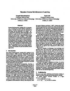
Figure 1 - Individual Starting-error Rates, T1 100%
% of population
75%
50% Phase II Phase III 25%
0% 0-10%
10-30%
30-50%
50-75% 75-100%
individual starting-error rates
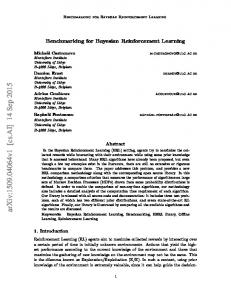
Figure 2 - Individual Switching-error Rates, T1
% of population
100%
75%
R, I-II-III LB, I-II LW, I-II L, III
50%
25%
0% 0-10%
10-30%
30-50%
50-75% 75-100%
individual switching-error rates
Figure 1 shows a great deal of variation in starting choices. Figure 2 shows that only a handful of participants make many (over 10%) switching errors after an initial RIGHT draw, as shown in the column to the far left of the chart. On the other hand, there is a wide spread (high variance across individuals) in switching-error rates after a draw from the LEFT. In Phase I-II, there are many individuals in each of the categories displayed; this is the case for both Black and White initial observations. In Phase III, there are only a few people who switch to RIGHT more than half the time, but there is still considerable variance across the first three categories. Thus,
17
there is broad consensus on updating after a RIGHT draw, but considerable variation in behavior after a LEFT initial draw.
Figure 3 - Individual Starting-error Rates, T2
% of population
100%
75%
50% Phase II Phase III 25%
0% 0-10%
10-30%
30-50%
50-75%
75-100%
individual starting-error rates
Figure 4 - Individual Switching-error Rates, T2
% of population
100%
75%
R, I-II-III LB, I-II LW, I-II L, III
50%
25%
0% 0-10%
10-30%
30-50%
50-75%
75-100%
individual switching-error rates
18
Figure 5 - Individual Switching-error Rates, T3
% of population
100%
75%
50%
F, I U, I All II
25%
0% 0-10%
10-30%
30-50%
50-75%
75-100%
individual switching-error rates
The patterns here are very similar to those in Treatment 1, with starting errors being a bit less common in Treatment 2.
Questions Q1. Do people follow the optimal switching rules? After starting from RIGHT the switching decision is simple, as the outcome fully resolves uncertainty regarding the state of Nature. Thus, the decision to stay with RIGHT both ‘feels’ right and is ‘rational’. Not surprisingly, we observe a very close correspondence between BEU-predictions and actual decisions when DMs start with RIGHT. The aggregate error rate after RIGHT draws is 4.4% in Treatment 1 and 5.3% in Treatment 2. Even this low proportion masks the fact that there are ‘worst offenders.’ In Appendix C we present tables that consider error rates excluding people who make abundant switching errors (or alternatively, any switching errors) after RIGHT. We exclude seven DMs as worst offenders in each of Treatments 1 and 2. These people, who constitute roughly 12% of the population (7/59 and 7/54), are responsible for
19
about 75% of all errors.12 Apart from those seven people, the aggregate error rate is between 1% and 2% in every category.13 After starting from LEFT the decision how to continue is much more complex. Again, drawing a Black (White) ball here means success (failure) and is likely to reinforce continuing drawing (switching to drawing) from the LEFT (RIGHT). However, even without precise (Bayes) calculations one may sense that here as well, as in RIGHT, observing a Black ball raises the likelihood that the state of nature is UP (DOWN), thus creating an incentive to switch to the RIGHT (stay with LEFT). These two opposite forces are not so easily resolved. Thus, we expected a higher error rate after starting from LEFT.14 In fact, what we see is a very different picture than with RIGHT initial draws. There is a rather poor correspondence between BEU-predictions and actual decisions; switching-error rates in Phase I and Phase II are substantial (between 34% and 59%) after LEFT draws, for both Treatments 1 and 2. Recall that in these earlier phases a BEU must switch after a success and not switch after a failure, the opposite of the prediction of a reinforcement or case-based model. The error rates in Phase III of Treatment 1, where a BEU should never switch from LEFT regardless of the 1st draw, are much lower than in the earlier phases, but are still substantial; in Treatment 2 these error rates are definitely higher, particularly after a black ball is drawn. Thus, the answer to Q1 depends on the starting side.
12
For example, the high error rate for Phase III after a Black draw in Treatment 1 reflects three DMs who made 16 of the 20 errors in this case. 13 This is about as good as it gets in laboratory tasks. A colleague points out that this is lower than the percentage of students who forget to write a name on the exam book after being reminded three times. 14 A careful reader may wish to keep in mind that the reinforcement forces after starting from LEFT may have a different impact on a DM in Phase I as compared to Phase II, due to the restriction on the initial draw. It seems plausible that the emotional reaction to the results of the first draw might be stronger when one has chosen LEFT voluntarily.
20
Q2. Are the switching-error rates the same after Black and White draws? After initial RIGHT draws in Treatment 1, the low aggregate switching-error rate is largely independent of whether the first draw was black or white. In contrast, when the 1st draw is from the LEFT in Phases I-II of Treatment 1, the error rate after drawing a black ball is nearly double the (still-substantial) error rate after drawing a white ball. For statistical purposes, we cannot treat each observation as being independent, so we must examine individual behavior. A Wilcoxon signed-ranks test (see Siegel and Castellan 1988) comparing each individual’s respective switching-error rates rejects the hypothesis that there is no difference in these switching-error rates, with Z = 3.08, p = 0.002 (two-tailed test). This large difference is also present when we exclude either worst offenders or all offenders. There is little difference in switching-error rates in Phase III of Treatment 1. There is a slight difference in switching-error rates after RIGHT draws in Treatment 2; however, this vanishes when the worst offenders are excluded.
In Phases I-II of Treatment 2,
the direction of the difference in switching-error rates after LEFT draws is reversed, with errors more common after observing a white ball than after observing a black ball. The Wilcoxon signed-ranks test again finds a significant difference between these switching-error rates, with Z = 2.01, p = 0.044 (two-tailed test). However, this difference is eliminated when we exclude the worst offenders, and seems to reverse slightly when we exclude all offenders. In Phase III, we see a very large difference in switching-error rates, which appears to actually increase when we remove subsets of offenders. The aggregate Phase I-II switching-error rate from LEFT in both Treatments 1 and 2 is close to 50%. Since ‘flipping a coin’ is often used as a metaphor for presenting one’s decision rule when clueless, one might be tempted to argue that this is the situation a DM finds himself
21
after drawing from the LEFT. However, a more careful examination reveals that this 50% aggregated switching-error rate is an artifact of the data. In Treatment 3, the switching-error rate after ‘unfavorable draws’ (different color than what is desired for the 2nd draw) in Phase I triple the corresponding rate after ‘favorable draws’ (same color as what is desired for the 2nd draw). On the other hand, there is only a modest difference between these rates in Phase II, where the payoffs have been reversed.
Q3. Is there any evidence that switching-error rates diminish over time? A natural consideration is whether the errors that we observe represent initial confusion or whether they generally persist through later periods. At a first rough cut, switching-error rates do not appear to diminishing over time. One comparison is between the first and second Phases of each Treatment. In Treatment 1, switching-error rates after RIGHT draws drop slightly from 4.9% in Phase I to 3.4% in Phase 2. However, the switching-error rate after LB actually increases from 53.6% in Phase I to 66.2% in Phase II. The rate does drop over slightly over time after LW. The overall error rate after starting with LEFT is slightly higher in Phase II than in Phase I (49.7% vs. 46.9%). However, since individuals make their initial choices voluntarily in Phase II and are forced to do so in Phase I, there is a self-selection issue that may confound comparisons across these phases. An alternative test of changes in behavior over time is to consider switching-error rates for time segments of the penultimate phase in each treatment, since the environment is constant for a relatively long interval. Table 4 shows these rates:
22
Table 4 – Switching Error Rates over Time Segments
Initial Draw RB RW LB LW
Initial Draw RB RW LB LW
Initial Draw F U
Treatment 1 Switching-error Rates Periods 21-30 Periods 31-40 5.0% 4.4% 60.4% 27.8%
2.5% 3.3% 61.4% 26.7%
Treatment 2 Switching-error Rates Periods 21-30 Periods 31-40 3.9% 0.5% 49.1% 49.2%
5.4% 2.3% 52.0% 54.3%
Treatment 3 Switching-error Rates Periods 1-20 Periods 21-50 13.4% 46.2%
13.9% 41.0%
Periods 41-50 2.6% 2.3% 77.8% 33.8%
Periods 41-50 5.4% 4.6% 58.0% 52.2%
Periods 51-70 13.1% 41.5%
The switching-error rate after RB decreases over time in both Treatments 1 and 2; however, while the rate after RW also increases over time in Treatment 1, it decreases over time in Treatment 2. In any case, all of these differences are rather small. The switching-error rate is either slightly increasing over time or is relatively flat after LEFT draws in all three treatments.15 Thus, overall we see little in the data to indicate that switching-error rates drop over time.
Starting decisions Let us next examine whether DMs make initial draws in accordance with the BEU model.
15
Since there are more Black draws than White draws from LEFT, and since the initial level of the LEFT switchingerror rates is higher for Black, we might expect the Black error rate to decrease more quickly than the White error rate. However, our results are not in accord with this expectation.
23
Q4. Do people make-errors in choosing a side for the first draw? First, recall that the correct BEU choice in Treatment 1 is to start from RIGHT in Phase II and to start from LEFT in Phase III; in Treatment 2, it is best to start with RIGHT at all times. Since our calculations were made assuming a risk-neutral BEU, an obvious natural question to is whether our reported errors here can be rationalized by having a risk-averse BEU. To address this concerns we repeated our calculations, assuming that the DM has a constant-relative-riskaversion (CRRA) utility of the form: u(x) = x1−ρ, where ρ ∈ [0,1) is the CRRA coefficient. We find that, in Treatment 1, a very high and unreasonable degree of CRRA is needed to rationalize reversal in Phase II and no CRRA is sufficient for this in Phase III.16 Table 5 shows voluntary initial draws in Phase II and III of Treatments 1 and 2:
Table 5 – Starting-error Rates Treatment
Phase
BEU-start
Error Rate
1 2 1 2
II II III III
R R L R
491/1770 (27.7%) 351/1620 (21.7%) 321/590 (54.4%) 201/540 (37.2%)
In Phase II of both Treatments 1 and 2, the strong majority of people choose RIGHT, in accordance with the BEU prediction, although LEFT is chosen more than 20% of the time.17 People are somewhat more likely to start with RIGHT in Treatment 2 than in Treatment 1, in accordance with the fact that black balls are relatively less prevalent in Treatment 2. Wilcoxon tests on individual tendencies find the difference to be only marginally significant for Phase II (Z 16
Similar conclusions follow for the calibration in Treatments 2 and 3 We can also examine whether people are more likely to start with RIGHT over time, by considering Phase II behavior. In periods 21-30 of Treatment 1, 413 of 590 starts (70.0%) were from RIGHT. This increased slightly to 426 of 590 starts (72.2%) in periods 31-40, and to 439 of 590 (74.4%) in periods 41-50. In periods 21-30 of Treatment 2, 426/540 starts (78.9%) were from RIGHT. This decreased very slightly to 420 of 540 starts (77.8%) in periods 31-40, and to 423 of 540 (78.3%) in periods 41-50. 17
24
= 1.26, p = 0.104), but quite significant for Phase III (Z = 2.32, p = 0.010). On the other hand, it is interesting to note that the error rates for Phase II initial draws are much lower than for the switching decisions. This is a bit puzzling, since calculating the correct initial side from which to draw involves solving the switching problem (from both sides). In our later discussion, we provide some possible explanations regarding how DMs who did so poorly on the switching decisions do so much better on this more difficult problem.
Cost and Frequency of Errors Q5. Does the cost of an error affect the frequency of the error?
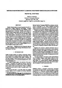
A natural question for economists is whether the frequency of decision errors is at least inversely related to the cost of such errors, even if complex BEU calculations may be beyond the ability of the general population. In fact, Table 6 and Figure 6 show that this is the case:
25
Table 6 – Cost and frequency of decision errors Error
EU of Choice
Size of Loss
% possible lost by error
Frequency of error
Treatment 1 Start Left, 21-50 Start Right, 51-60 Left after R, Black, 1-50 Right after R, White, 1-50 Right after L, White, 1-50 Left after L, Black, 1-50 Left after R, Black, 51-60 Right after R, White, 51-60 Right after L, White, 51-60 Right after L, Black, 51-60
87/72 93/72 2/3 0 7/15 25/42 7/9 0 2/5 4/7
15/72 (.208) 5/72 (.069) 1/2 (.500) 1/2 (.500) 7/36 (.194) 1/14 (.071) 2/9 (.222) 7/12 (.583) 47/180 (.261) 31/252 (.123)
14.7% 5.1% 42.9% 100.0% 29.4% 10.7% 22.2% 100.0% 39.5% 18.3%
.277 .544 .047 .039 .338 .594 .124 .044 .197 .152
Treatment 2 Start Left, 21-50 Start Left, 51-60 Left after R, Black, 1-50 Right after R, White, 1-50 Right after L, White, 1-50 Left after L, Black, 1-50 Left after R, Black, 51-60 Right after R, White, 51-60 Right after L, White, 51-60 Left after L, Black, 51-60
10/9 127/108 2/3 0 7/18 5/9 7/9 0 1/3 35/54
2/9 (.222) 1/54 (.019) 1/2 (.500) 1/3 (.333) 1/18 (.056) 2/9 (.222) 2/9 (.222) 7/18 (.389) 5/27 (.185) 1/54 (.019)
16.7% 1.6% 42.9% 100.0% 12.5% 28.6% 22.2% 100.0% 35.7% 2.8%
.217 .372 .070 .031 .542 .412 .112 .019 .294 .697
Treatment 3 Right after L, ‘White’, 1-70 Left after L, ‘Black’, 1-70 Right after L, ‘White’, 71-80 Left after L, ‘Black’, 71-80
7/18 5/9 1/3 35/54
1/18 (.056) 2/9 (.222) 5/27 (.185) 1/54 (.019)
12.5% 28.6% 35.7% 2.8%
.414 .134 .368 .301
26
Figure 6 - Cost and Frequency of errors 0.75 0.60 0.45 0.30 0.15 0.00 0
0.1
0.2
0.3
0.4
0.5
0.6
Cost of error
While the relationship is not completely smooth, it is clear that the higher the cost of an error, the less likely it is to be made. Every error that costs more than .30 has a frequency of less than 5%, while every error that costs less than .30 has a frequency greater than 11.2%. We perform simple OLS regressions on these data to examine the frequency of an error as a function of its cost:
Adjusted R2 = .6243
Frequency of error = 0.395 - 0.635*cost of error (11.4)
(-6.39)
Frequency of error = 0.474 – 1.441*cost of error + 0.120*cost2 (11.1)
(-4.62)
Adjusted R2 = .7047
(2.69)
The t-statistics are in parentheses and are all highly significant. These confirm the strong inverse relationship seen in the graph.
27
Gender Q6. Are there differences in error rates across gender? We have seen that there is considerable heterogeneity in the population. Can we find any determinants for this – specifically, are there any differences in behavior across gender? The motivation for such an inquiry is the possibility that females and male are responding with systematic differences to different triggers, the reinforcement response and the forward and rational reaction to the (pure) informational signal upon observing the color of the first draw. Table 7 shows male and female error rates:
28
Table 7 – Error Rates by Gender Error
Size of Loss
Male Error Rate
Female Error Rate
Difference
Wilcoxon Test Z
Treatment 1 Start Left, 21-50 Start Right, 51-60 Left after R, Black, 1-50 Right after R, White, 1-50 Right after L, White, 1-50 Left after L, Black, 1-50 Left after R, Black, 51-60 Right after R, White, 51-60 Right after L, White, 51-60 Right after L, Black, 51-60
.208 .069 .500 .500 .194 .071 .222 .583 .261 .123
.251 .523 .018 .020 .291 .611 .029 .000 .028 .094
.298 .561 .052 .053 .371 .585 .194 .076 .337 .203
-.047 -.038 -.034 -.033 -.080 .026 -.165 -.076 -.309 -.109
-1.28 -0.12 -0.07 -1.85* -1.41 -0.11 -0.98 -1.72* -0.37 -2.91***
Treatment 2 Start Left, 21-50 Start Left, 51-60 Left after R, Black, 1-50 Right after R, White, 1-50 Right after L, White, 1-50 Left after L, Black, 1-50 Left after R, Black, 51-60 Right after R, White, 51-60 Right after L, White, 51-60 Left after L, Black, 51-60
.222 .019 .500 .333 .056 .222 .222 .389 .185 .019
.180 .391 .056 .005 .438 .299 .159 .015 .233 .744
.242 .359 .081 .046 .608 .479 .083 .021 .339 .661
-.062 .032 -.025 -.041 -.170 -.180 .076 -.006 -.106 .083
-1.04 -0.78 -0.85 -1.30 -1.95** -2.02** 0.31 -0.31 -0.12 -0.06
Treatment 3 Right after L, ‘White’, 1-70 .056 .397 .445 -.048 -0.52 Left after L, ‘Black’, 1-70 .222 .065 .194 -.129 -2.88*** Right after L, ‘White’, 71-80 .185 .300 .302 -.002 -0.56 Left after L, ‘Black’, 71-80 .019 .277 .458 -.181 -0.25 *significant at p = 0.10 (two-tailed test) ** significant at p = 0.05 *** significant at p = 0.01 We use the Wilcoxon-Mann-Whitney ranksum test on individual error rates, with around 25-30 individuals of each gender for each comparison. Ranksum tests have the advantage of implicitly putting less weight on outliers, since a very high error rate for an individual translates only into a poor ranking. Thus, some of the apparently large differences that are due to outliers are not significant.
29
While only a few of the comparisons are significant on an individual basis, there does seem to be a pattern here. The female error rate is higher is 20 of the 24 comparisons.18 A binomial test thus rejects equality at p = 0.002, two-tailed test. In addition, the difference seems to be sharper when errors are more costly. For the 12 costliest errors of the 24 listed (cost at least .222), male error rates were lower in 11 cases, with the single exception being at the lowest cost in the range. Five of these 12 differences were at least marginally significant. Aggregated over treatments, 36 (70.6%) of the 51 male participants made no switching errors after initial RIGHT draws; this compares with 33 (53.2%) of the 62 female participants. The difference in the proportions of error-free draws after a RIGHT initial draw is marginally significant (Z = 1.88, p = 0.065, two-tailed test). It would appear that the reinforcement heuristic is relatively stronger for the female participants in our study.
IV. Discussion On a basic (or even evolutionary) level, reinforcement seems a simple and natural mechanism for living organisms to use for guidance and learning, since no elaborate cognitive process is needed. Even simple living mechanisms, once equipped with a utilitarian/hedonistic capacity, can be guided to increase the frequency of choices and actions that align with that hedonistic capacity, serving as an effective proxy for Nature’s grand design. In contrast, the ability to update priors, even if in an imperfect (Bayesian) way seems to require enormously more: brain, reasoning, cognition, etc.
However, good quality solutions to many decision
problems in general, and economic ones in particular, require one to update priors when new information arrives. 18
The observant reader will notice that 23 of the 24 signs for the nonparametric tests are negative, an even stronger result. Apparently three of the cases where the difference was positive were so outlier-driven that the rank-sum test
30
A sophisticated DM when confronted with a decision problem framed in terms of priors and additional information (as in our experiment) may recognize the environment and apply some updating heuristics (Bayesian if he or she is a good student of decision theory). But how likely is it that in a real life (and unframed) situation a less-than-fully-sophisticated DM will indeed apply something close to Bayes’ rule? distinction is all that important.
Another relevant question is whether this
One might question whether decisions where these two
heuristics clash are very common. We suspect that in most situations both heuristics are at least partially aligned, so that relying on reinforcement alone may be effective. Nevertheless, our results indicate that both heuristics are at work, and that when they clash we can expect confusion and divergence from optimality. We feel that this observation provides an important insight. We suspect that there tends to be at least a kernel of updating from negative inferences in many decisions. In any case, even if reinforcement and Baysian updating often give the same advice, we argue that observing the results of this clash and the relative strengths of the conflicting forces may help to explain differential intensities of certain behaviors even when they do not clash. In some cases, DMs experience both forces, while others are experiencing only one. Consider, for example, an investor whose recent portfolio has performed very well, beyond investor expectations. Choi, Laibson, Madrian & Metrick (2003) find the puzzling result that people who experience orthogonal positive wealth shocks (higher appreciation than expected) in their 401k retirement accounts do not increase their consumption, in violation of standard theory. As differences in capital gains in one’s own portfolio vs. capital gains in another investor’s portfolio should be irrelevant for forecasting future returns, in principle the informational content of the recent idiosyncratic success can be ignored.
gives them them a negative (but not significant) test statistic.
31
However, in practice this does not appear to be the case. Since future returns on any given portfolio are equally available to all investors and information about past returns is public, one might wonder why these two investors appear to process information differently, as seems to be implied by their results. In terms of our work, an explanation might be that the affect of a successful choice gives an additional ‘push’ for successful investors to invest in the 401(k). We would further conjecture that investors who personally select their own 401k portfolios would be particularly prone to this influence. Some evidence relevant to this conjecture emerges from our study, as we can test this point by comparing switching decisions after voluntary and involuntary initial draws.
A
successful portfolio (black, in Treatments 1 and 2) can be the outcome of ‘investing’ in either RIGHT or LEFT. Successful investors in RIGHT will continue to invest in RIGHT, as would any observer learning the outcome of the draw. However, a successful investor in LEFT who has elected to invest initially in LEFT (Phase II) is more likely to invest in LEFT in the next draw than is the investor who has also had a good outcome, but did not choose where to invest (Phase I). LB switching rates are about 12 percentage points higher in Phase II than in Phase I in both Treatment 1 and Treatment 2. This difference corresponds to about a 20-25% increase. On the other hand, switching errors after LW draws in fact decrease slightly from Phase I to Phase II, in both treatments. Thus, DMs who observe a white ball after an initial LEFT draw are more likely to persist with LEFT for the 2nd draw when the first LEFT draw was voluntary. In terms of the portfolio story, this means that an investor who chooses a portfolio tends to invest more in it after a bad outcome than does an investor who has observed the outcome without personal involvement. We do not find that increasing the precision of the information received after a LEFT draw reduces the switching-error rate (Hypothesis 1). On the other hand, we find evidence that 32
removing the affect from ‘winning’ on the 1st draw (Treatment 3) reduces errors, as average error rates in Treatment 3 are indeed considerably lower (Hypothesis 3).
Finally, it is perhaps
reassuring that when LEFT is made less attractive (by changing the composition of the balls in the LEFT urn in the UP state), the LEFT choice is always less frequent in starting and in switching decisions. We do find a strong relationship between the cost and frequency of errors. However, if the cost of error is the primary consideration, one might expect that error rates diminish over time, as people tried to avoid these costs.
Yet we find little or no evidence that error rates
decrease over time, as one might expect with some form of reinforcement learning. In fact, our results go to the question of the nature of reinforcement. On the one hand, the reinforcement from payoffs does not appear to be a major factor, given the lack of change over time. On the other hand, we see a strong influence from affect, which could be considered reinforcement on a more visceral level. Since this affect seems to play such a large role, it would appear that reinforcement models might be improved by considering the affective reward as part of the overall ‘payoff’. Regarding initial draws, there seems to be a pronounced tendency to prefer to make the first draw from the RIGHT, unrelated to BEU calculations. In Treatment 1, this is selected 72% of the time in Phase II (when it is correct under BEU) and 54% of the time in Phase III (when it is not correct under BEU). In Treatment 2, RIGHT is selected first 78% of the time in Phase II (when it is correct under BEU) and 63% of the time in Phase III (when the expected payoff is nearly the same for RIGHT and LEFT starts).19 Perhaps one explanation for this behavior can be traced to the fact that making the first draw from the RIGHT leads to easy subsequent
19
This 63% figure is perhaps the clearest evidence of the start-from-RIGHT bias, since the expected (optimal) payoffs from starting with either urn are nearly identical.
33
switching decisions. In contrast, starting from LEFT leads to a difficult decision node after the first draw; this is true both conceptually and as evidenced by the data. We see at least two plausible explanations for this phenomenon. First, there may be a ‘curiosity effect’; people express interest in learning whether the actual state in the period was Up or Down.
Making at least one choice from RIGHT ensures that the DM learns this
information, while LEFT choices leave this question unanswered. Second, a DM who selects LEFT initially and then gets a bad outcome on the next draw might at that point be haunted by the suspicion that he or she updated incorrectly and was therefore instrumental with respect to the bad outcome. Loomes and Sugden (1982) introduce the notion of regret in choice under uncertainty. If an individual chooses between two actions and the outcome resulting from her choice is less desirable than the outcome that would have resulted (in the ex post state of the world) from the other action, this may serve to diminish the pleasure that the individual might otherwise receive from the less desirable outcome.20 In our context, this could lead to regret over the initial choice. To the extent that DMs anticipate or experience this, first draws from RIGHT become more likely. The second explanation ties in with the notion of ‘complexity aversion’ (Sonsino and Mandelbaum, 2001) and with having a preference for avoiding cognitive dissonance.21 In our context, participants are quite likely to be unclear about the BEU updating after a LEFT draw. People prefer to avoid environments where the cognitive burden is high or even beyond their capability, as poor outcomes lend themselves to the unpleasantness of cognitive dissonance. Regarding switching decisions, we find that there seems to be a reluctance to switch when the first draw is from LEFT, since the error rate is much higher when one is supposed to 20
The authors motivate the concept by pointing to the difference between the sensation of losing a sum of money at a horse race and the sensation of losing the same sum as the result in income tax rates.
34
update and switch (black draw) than when one is supposed to update and stay (white draw). People who voluntarily start with LEFT (in Phase II) tend to ‘stick to their guns’ and not switch more frequently than when they are constrained to start with LEFT (Phase I). This suggests that there is less updating in this more complex cognitive task than in the simpler one after starting with RIGHT, where the switching patterns closely match the predictions. Note that this contrasts with Grether (1980), who finds that “individuals tend to give too much weight to the ‘evidence’ and thus too little weight to their prior beliefs, though priors are not ignored.” Perhaps the fact that the first ‘draw’ contained information, but no affective element, can help reconcile this difference.
In any case, this behavior seems entirely consistent with the status quo bias
(Samuelson and Zeckhauser 1988), which predicts that people are reluctant to make changes when risky outcomes are involved. Another possible explanation for such different error rates (switching behavior after success vs. after failure) beyond differential cost of errors that we discuss below would be that positive reinforcement affects behavior more than negative reinforcement does – “carrots are more effective than sticks”.
However, it is far from clear that this is the case.
In fact,
Baumeister, Bratslavsky, Finkenauer & Vohs (2001) discuss the pervasive evidence that “bad is stronger than good.”
Nevertheless, our results in Treatment 3 strongly suggest that
psychological affect plays a major role in switching decisions, and that positive affect is a stronger motivational force than negative affect; while removing affect from initial LEFT draws reduces the error rate after ‘black’ (favorable) draws by 63% (from 36.8% in Phase I of Treatment 2 to 13.5% in Treatment 3), the corresponding reduction in the error rate after ‘white’ (unfavorable) draws is only 24% (from 55.7% to 42.4%).
21
This complexity aversion is not what is referred in the literature as ambiguity or uncertainty aversion where a DM is uncertain about relevant probability distributions. See for example Camerer and Weber (1992, p. 330).
35
V. Conclusion We conduct an experiment that permits us to compare the motivating force of BEU to that of reinforcement (or case-based) learning. The heart of our design is to construct situations where these two motivations are aligned and situations where they conflict. Our results indicate that both heuristics are at work, and that when they clash we can expect divergence from BEU. We believe that examining the relative strengths of the conflicting forces is useful for explaining differential intensities of behavior even when the forces do not clash. When BEU predictions agree with those of reinforcement/case-based decision theory models, nearly all people respond as expected. However, there is a mixture of behavior when these predictions point in opposing directions. Nearly 50% of all switching decisions after LEFT draws violate the Bayes updating rule in Treatments 1 and 2; this drops substantially in Treatment 3, where the LEFT initial draw is stripped of its affect. It appears that much of the power of reinforcement comes from the psychological affect induced by an outcome, rather than from a more cortical consideration of one’s received payoffs. We find evidence of a preference for simplicity, as exemplified by a start-from-RIGHT bias. Choosing to choose a ball from the clearer environment helps the decision-maker avoid potential regret and cognitive dissonance. We also observe that people seem to be reluctant to switch urns for their second draw, particularly when there is affect involved. This reluctance to switch is stronger when the decision-maker has the opportunity to decide the urn from which to make the initial choice. This behavior is consistent with the Samuelson and Zeckhauser (1988) status quo bias. Our initial foray into this area leaves much more work to be done, and we plan to pursue this rich vein. One area concerns differences in individual behavior. With better controls on 36
individual background (beyond gender), one could assess the roles that age, education level and sophistication (e.g., math and stat background) play in the weights assign to the different heuristics when they clash. Another conjecture that emerges and can be tested is that lower animals, say rats, would have even higher switching error rates from LEFT. Finally, in our design, the simple errors (i.e., incorrect updating after a RIGHT draw) are the most costly. It should be interesting to see what happens when the simpler decision errors are not so costly (in expectation), while decision errors in more complex environments are relatively expensive. We suspect that the cost of the error is not the true independent variable, as people are hardly calculating the cost of an error and then choosing how careful to be.
References Baumeister, R., E. Bratslavsky, C. Finkenauer & K. Vohs (2001), “Bad is Stronger than Good,” Review of General Psychology, 5, 323-370. Camerer, C. and T. Ho (1998), “Experience-Weighted Attraction in Games: Estimates from Weak-link Games,” in D. Budescu and R. Zwick,editors, Games and Human Behavior, Essays in Honor of Amnon Rapaport, 31-53, Hillsdale: NJ. Camerer, C. and T. Ho (1999), “Experience-Weighted Attraction Learning in Games: A Unifying Approach,” Econometrica, 67, 827-874. Camerer, C. and M. Weber (1992), “Recent Developments in Modeling Preferences: Uncertainty and Ambiguity,” Journal of Risk and Uncertainty, 5, 325-370. Choi, J., D. Laibson, B. Madrian & A. Metrick (2003), “The Marginal Propensity to Consume Out of Retirement Wealth Shocks is Weakly Negative,” mimeo. Cheung, Y. and D. Friedman (1997), “Individual Learning in Normal Form Games: Some Laboratory Results,” Games and Economic Behavior, 19, 46-76. Erev, I. and A. Roth (1998a), “Predicting How People Play Games: Reinforcement Learning in Experimental Games with Unique, Mixed Strategy Equilibria,” American Economic Review, 88, 848-881. Erev, I. and A. Roth (1998b), “On the Role of Reinforcement Learning,” in D. Budescu and R. Zwick, eds, Games and Human Behavior, Essays in Honor of Amnon Rapaport, Hillsdale: NJ. Fudenberg, D. and D. Levine (1998), The Theory of Learning in Games,” MIT Press: Cambridge, MA.
37
Gilboa, I and D. Schmeidler (1995), “Case-Based Decision Theory,” Quarterly Journal of Economics, 110, 605-639. Gilboa, I and D. Schmeidler (2001), A Theory of Case-Based Decisions, Cambridge: Cambridge University Press. Grether, D. (1980), “Bayes Rule and the Representativeness Heuristic: Some Experimental Evidence,” Journal of Economic Behavior and Organization, 17, 31-57. Grether, D. (1992), “Testing Bayes Rule as a Descriptive Model: The Representativeness Heuristic,” Quarterly Journal of Economics, 95, 537-557. Kahneman, D. and A. Tversky (1972), “Subjective Probability: A Judgment of Representativeness,” Cognitive Psychology, 3, 430-454. Loomes, G. and R. Sugden (1982), “Regret Theory: An Alternative Theory of Rational Choice Under Uncertainty,” Economic Journal, 92, 805-824. Ouwersloot, H., P. Nijkamp & P. Rietveld (1998), “Errors in Probability Updating Behaviour: Measurement and Impact Analysis,” Journal of Economic Psychology, 19, 535-563. Roth, A. and I. Erev (1995), “Learning in Extensive-form Games: Experimental Data and Simple Dynamic Models in the Intermediate Term,” Games and Economic Behavior, 8, 164-212. Samuelson, W. and R. Zeckhauser (1988), “Status Quo Bias in Decision-Making,” Journal of Risk and Uncertainty, 1, 7-59. Sonsino, D. and M. Mandelbaum (2001), On Preference for Flexibility and Complexity Aversion: Experimental Evidence,” Theory and Decision, 51, 197-216. Suppes, P. and R. Atkinson (1960), Markov Learning Models for Multiperson Interaction, Stanford University Press, Palo Alto, CA. Tversky, A. and D. Kahneman (1971), “Belief in the Law of Small Numbers,” Psychological Bulletin, 76, 105-110. Tversky, A. and D. Kahneman (1973), “Availability: A Heuristic for Judging Frequency and Probability,” Cognitive Psychology, 5, 207-232. Zizzo, D, S. Stolarz-Fantino, J. Wen & E. Fantino (2000), “A Violation of the Monotonicity Axiom: Experimental Evidence on the Conjunction Fallacy,” Journal of Economic Behavior and Organization, 41, 263-276.
38
APPENDIX A
SUPPLEMENTAL INSTRUCTIONS
Decision task Think of your decision task as consisting of drawing colored balls from urns. There are two urns (LEFT and RIGHT) from which the individual can draw balls, and there are two equally likely states of the world (UP and DOWN). The urns contain some combination of black balls and white balls. In state UP, the LEFT urn has 4 black balls and 2 white balls and the RIGHT urn as 6 black balls. In state DOWN, the LEFT urn has 3 black balls and 3 black balls, while the RIGHT urn has 6 white balls. You get paid for drawing black balls. You make a draw from either the LEFT or the RIGHT urn in the 1st decision in the period, and then this ball is put back into the urn. You then make a 2nd draw from either the LEFT or the RIGHT urn, knowing that if the state was UP (or DOWN) for the first draw, it is also UP (or DOWN) for the 2nd draw. There will be 60 periods in this experiment, in blocks of 10. There are two draws in each period. A critical point is that it is the same state (UP or DOWN) for both of these draws. In the first 50 periods (100 draws), you get paid 30 cents for each black ball drawn from the LEFT urn and 35 cents for each black ball drawn from the RIGHT urn. In the last 10 periods, this is reversed: you will be paid 35 cents for each black ball drawn from the LEFT urn and 30 cents for each black ball drawn from the RIGHT urn. In the first 20 periods, you are restricted for your first draw. In some periods, you must make your 1st draw from the LEFT urn and in other periods you must make your 1st draw from the RIGHT urn. You are never restricted as to your 2nd draw in the period. On the computer, we don’t have actual urns. We simulate this by having 6 cards on the LEFT side and 6 cards on the RIGHT side. You will pick one of the cards (on whichever side you wish, subject to the constraint on the 1st draw for the 1st 20 periods), learn the outcome, and the card is replaced (with the 6 cards on that side re-shuffled). You then make the 2nd draw for the period and learn the outcome. We then move to the next period. The experimental instructions are on the computer screen, but hopefully these supplemental instructions are helpful. Any questions?
39
APPENDIX B AN EXAMPLE OF EXPECTED UTILITY CALCULATIONS With two draws in Phase I or Phase II of Treatment 1, first suppose that RIGHT is chosen on the first draw. Then the expected utility of both draws is 17/12: EU (both draws) =
1 7 7 1 1 17 × + + = 2 6 6 2 2 12
The reasoning is that if a black ball is drawn, the state is UP, so the DM again selects the RIGHT urn on the 2nd draw. However, if a white ball is drawn, the state is DOWN, so that the DM switches to LEFT, with a probability of 1/2 of drawing a black ball on the 2nd draw. On the other hand, suppose LEFT is chosen on the first draw. The expected utility of the 1st draw is 7/12, as before. Note that Pr[UP|black] = 4/7 and that Pr[UP|white] = 2/5. Suppose the 1st ball drawn is black; this occurs with a probability of 7/12. Then, 4 2 3 1 25 EU ( LEFT on 2nd draw) = × + × = 7 3 7 2 42
However, EU(RIGHTon 2nd draw) =
4 7 28 × = 7 6 42
Thus, if the DM draws a black ball from the LEFT urn on the 1st draw, it is optimal to switch to the RIGHT urn for your 2nd draw. Now instead suppose that the 1st ball drawn is white; this occurs with a probability of 5/12. Then, 2 2 3 1 17 EU ( LEFT on 2nd draw) = × + × = 5 3 5 2 30
and 2 14 3 14 EU(RIGHTon 2nd draw) = × + ×0 = 5 12 5 30
Thus, if a white ball is drawn from the LEFT urn on your 1st draw, it is optimal to stay with the LEFT urn on your 2nd draw. So after starting start with LEFT, EU(both draws) =
7 7 28 5 17 87 = + × + × 12 12 42 12 30 72
Since 87/72 < 102/72 = 17/12, starting with RIGHT is optimal when there are two draws.
40
APPENDIX C – Individual Behavior INDIVIDUAL ERROR RATES, STUDY 1 Gender F
SE, II 0.03
SE, III 0.80
LB, I-II 0.63
LB, III 0.00
LW, I-II 1.00
LW, III 0.00
All L, III 0.00
RB, I-II 0.00
RB, III 0.00
RW, I-II 0.00
RW, III 0.00
All R, III All R, I-III 0.00 0.00
M M M M F F M M M F F M
0.00 0.00 0.00 0.00 0.10 0.20 0.00 0.00 0.03 0.60 0.13 0.43
1.00 0.00 1.00 1.00 0.10 0.80 1.00 1.00 0.00 0.10 0.00 0.30
0.14 1.00 0.00 0.00 0.17 0.13 0.71 0.00 0.00 0.94 0.50 0.31
0.00 0.00 1.00 0.00 0.00 0.00 0.00
0.67 0.00 0.17 1.00 0.71 0.88 0.67 0.00 1.00 0.00 0.63 0.71
0.00 0.50 0.00 0.00 0.00 0.00 0.25
0.00 0.11 0.50 0.00 0.00 0.00 0.14
0.00 0.00 0.00 0.00 0.00 0.00 0.00 0.00 0.00 0.00 0.00 0.00
0.00 0.20 0.00 0.00 0.00 0.00 0.00 0.50
0.00 0.00 0.00 0.00 0.04 0.06 0.00 0.00 0.00 0.00 0.00 0.00
0.00 0.00 0.00 0.25 0.00 0.00 0.00 0.00
0.00 0.10 0.00 0.00 0.13 0.00 0.00 0.00 0.33
0.00 0.00 0.02 0.00 0.03 0.05 0.00 0.00 0.00 0.00 0.00 0.03
M M F F M M M M M F M M
0.00 0.00 0.07 0.63 0.40 0.47 0.47 0.87 0.70 0.57 0.03 0.60
0.90 1.00 0.90 0.00 0.70 0.00 0.00 0.10 0.00 0.50 1.00 0.30
0.25 0.20 0.50 0.00 0.50 0.85 0.00 1.00 1.00 0.69 1.00 1.00
0.88 0.00 0.00 0.00 0.00 0.00 0.50 0.00
0.50 0.20 0.50 0.06 0.40 0.82 0.33 0.00 0.00 0.36 0.00 0.50
1.00 0.00 0.00 0.50 0.00 0.25 0.00 0.00 0.00 -
1.00 0.00 0.70 0.33 0.00 0.10 0.00 0.00 0.20 0.00
0.00 0.05 0.00 0.00 0.00 0.44 0.00 0.00 0.00 0.50 0.00 0.00
0.00 0.00 0.00 0.00 0.00 0.50 0.00 0.00
0.00 0.00 0.06 0.00 0.14 0.29 0.00 0.00 0.00 0.55 0.00 0.09
0.00 0.00 0.00 0.00 0.33 0.00 0.00
0.00 0.00 0.00 0.00 0.00 0.40 0.00 0.00
0.00 0.02 0.02 0.00 0.06 0.35 0.00 0.00 0.00 0.50 0.00 0.04
F F F M F
0.27 0.20 0.33 0.50 0.27
0.60 0.40 0.80 0.50 0.60
0.08 0.75 0.54 0.56 0.73
1.00 0.60 1.00 0.00 0.00
0.33 0.50 0.29 0.22 0.43
0.00 1.00 0.00 0.00
1.00 0.50 1.00 0.00 0.00
0.00 0.05 0.00 0.00 0.00
0.00 0.00 1.00 0.00 0.00
0.00 0.17 0.00 0.00 0.00
0.00 0.00 0.00 0.00 0.00
0.00 0.00 0.75 0.00 0.00
0.00 0.08 0.16 0.00 0.00
F F F F M F F
0.17 0.17 0.17 0.03 0.00 0.43 0.27
0.40 0.80 0.80 1.00 0.00 0.70 0.60
0.50 0.50 0.80 0.80 0.86 0.83 0.27
1.00 0.00 0.00 0.00
0.43 0.67 0.60 0.50 0.33 0.36 0.14
0.75 0.50 0.50 0.00 0.00 0.00
0.83 0.50 0.50 0.00 0.00 0.00
0.76 0.00 0.00 0.00 0.08 0.00 0.00
0.00 0.00 0.00 0.00 0.00
0.28 0.00 0.00 0.00 0.00 0.07 0.00
0.00 0.00 0.00 0.00 0.00 0.00
0.00 0.00 0.00 0.00 0.00 0.00
0.46 0.00 0.00 0.00 0.03 0.03 0.00
F M M F F F F M F F M M
0.03 0.53 0.30 0.17 0.20 0.13 0.00 0.40 0.27 0.83 0.27 0.53
0.00 0.00 0.60 0.90 0.10 1.00 1.00 0.60 1.00 1.00 0.60 0.00
0.80 0.93 0.45 0.50 0.91 0.86 0.00 0.64 0.30 0.95 0.22 0.93
0.17 0.00 0.00 0.40 0.00 1.00 0.00
0.17 0.00 0.25 0.43 0.40 0.43 0.00 0.55 0.13 0.47 0.11 0.00
0.00 0.00 0.00 0.00 0.50 1.00 0.00 0.00
0.10 0.00 0.00 0.00 0.44 0.25 0.50 0.00
0.00 0.00 0.06 0.00 0.00 0.13 0.00 0.00 0.00 0.00 0.00 0.00
0.00 0.00 0.67 0.00 0.00 0.00 1.00 0.00 -
0.00 0.00 0.00 0.00 0.00 0.00 0.00 0.00 0.00 0.25 0.00 0.00
0.00 0.00 0.00 0.00 0.25 0.00 0.00 1.00 0.00 -
0.00 0.00 0.00 0.40 0.10 0.00 0.00 1.00 0.00 -
0.00 0.00 0.03 0.00 0.00 0.13 0.02 0.00 0.00 0.48 0.00 0.00
F M F F F F F M F F
0.90 0.00 0.00 0.50 0.77 0.03 0.53 0.00 0.50 0.33
0.00 1.00 1.00 0.50 0.00 1.00 0.50 1.00 0.10 0.50
1.00 0.00 0.75 0.69 0.16 0.80 0.82 1.00 0.27 0.45
0.00 0.00 0.57 0.25 0.25 0.00
0.00 0.00 0.83 0.33 0.00 0.67 0.67 0.00 0.40 0.44
0.00 0.00 0.00 1.00 1.00 0.33
0.00 0.00 0.40 0.40 0.33 0.20
0.00 0.00 0.00 0.33 0.00 0.00 0.00 0.00 0.00 0.00
0.00 0.00 0.00 0.00 0.00 0.00 1.00 0.00
0.00 0.00 0.04 0.06 0.00 0.00 0.00 0.00 0.56 0.00
0.00 0.00 0.00 0.00 0.00 0.00 0.00
0.00 0.00 0.00 0.00 0.00 0.00 1.00 0.00
0.00 0.00 0.02 0.13 0.00 0.00 0.00 0.00 0.38 0.00
1
INDIVIDUAL ERROR RATES, STUDY 2 Gender F
SE, II 0.23
SE, III 0.00
LB, I-II 0.00
LB, III 0.00
LW, I-II 0.00
LW, III 0.00
All L, III 0.00
RB, I-II 0.00
RB, III -
RW, I-II 0.00
RW, III -
All R, III -
All R, I-III 0.00
F M F F F F F F F M F F
0.00 0.33 0.00 0.40 0.00 0.07 0.53 0.00 0.67 0.00 0.40 0.13
0.20 0.40 0.60 0.40 0.60 0.70 0.20 0.20 0.10 0.40 0.50 0.30
0.00 0.30 1.00 1.00 0.80 0.00 0.67 0.50 0.14 0.00 0.67 0.80
1.00 0.50 1.00 0.80 0.00 1.00 0.00
0.00 0.40 1.00 1.00 0.80 0.00 1.00 0.75 0.94 0.14 0.50 0.44
0.50 1.00 1.00 0.25 0.00 0.00 0.38
0.60 0.75 1.00 0.56 0.00 0.67 0.33
0.00 0.00 0.00 0.00 0.00 0.00 0.00 0.00 0.75 0.00 0.00 0.00
0.00 0.00 0.00 0.00 0.00 1.00 0.00 1.00 0.00 0.00 -
0.00 0.08 0.00 0.13 0.00 0.00 0.07 0.00 0.58 0.05 0.00 0.05
0.00 0.00 0.00 0.00 0.00 0.00 0.00 0.00 0.17 0.00 0.00
0.00 0.00 0.00 0.00 0.00 0.00 1.00 0.00 0.50 0.10 0.00 0.00
0.00 0.03 0.00 0.06 0.00 0.00 0.08 0.00 0.64 0.04 0.00 0.03
M F F F M M F F F M M M
0.00 0.00 0.03 0.27 0.00 0.50 0.00 0.00 0.23 0.03 0.03 0.00
0.70 0.80 0.40 0.70 0.50 0.40 0.60 0.30 0.10 0.00 0.60 0.10
0.25 0.00 0.00 0.22 0.00 0.77 0.00 0.25 0.27 0.33 0.20 0.00
1.00 1.00 1.00 1.00 0.00
1.00 0.67 0.60 1.00 1.00 0.33 0.71 0.83 0.17 0.38 0.33 0.00
1.00 0.50 0.00 0.00 0.25
1.00 0.60 0.60 0.50 0.10
0.00 0.00 0.00 0.42 0.00 0.00 0.00 0.00 0.00 0.00 0.05 0.00
0.29 0.75 0.00 0.00 0.00 0.00 0.00 0.00 1.00 0.00 -
0.00 0.00 0.06 0.46 0.00 0.00 0.05 0.00 0.00 0.00 0.00 0.00
0.00 0.00 0.00 0.50 0.00 0.00 0.00 0.00 0.00 0.00 -
0.20 0.60 0.00 0.17 0.00 0.00 0.00 0.00 0.20 0.00 -
0.04 0.12 0.02 0.42 0.00 0.00 0.02 0.00 0.03 0.00 0.02 0.00
M F F F M F
0.33 0.03 0.00 0.07 0.07 0.43
0.50 0.70 0.50 0.10 0.30 0.50
0.75 0.33 1.00 0.00 0.00 0.18
1.00 0.67 1.00
0.17 0.88 0.00 0.50 0.33 0.25
1.00 0.17 0.00 0.00
1.00 0.33 0.00 0.33
0.00 0.00 0.00 0.04 0.00 0.00
0.00 0.00 0.00 0.67 0.00
0.00 0.00 0.28 0.15 0.00 0.00
0.00 0.00 0.00 0.00 0.00 0.00
0.00 0.00 0.00 0.00 0.29 0.00
0.00 0.00 0.10 0.08 0.04 0.00
2
F F M M M F M
0.63 0.03 0.07 0.70 0.00 0.37 0.00
0.20 0.60 0.50 0.50 0.50 0.30 0.10
0.75 0.00 0.25 0.00 0.00 0.67 0.00
1.00 0.75 1.00
0.65 1.00 0.13 0.55 0.00 0.33 0.20
0.00 0.00 0.00 0.00 0.00
0.60 0.00 0.00 0.43 0.71
0.00 0.88 0.00 0.00 0.00 0.00 0.00
0.00 0.00 0.00 0.00 0.00 0.00 0.00
0.00 0.00 0.00 0.00 0.00 0.00 0.00
0.00 0.00 0.00 0.00 0.00 0.00
0.00 0.00 0.00 0.00 0.00 0.00 0.00
0.00 0.31 0.00 0.00 0.00 0.00 0.00
M M M F F M M M M F F F
0.00 0.13 0.60 0.27 0.20 0.23 0.23 0.47 0.23 0.40 0.90 0.53
0.30 0.00 0.30 0.40 0.40 0.40 0.20 0.40 0.60 0.30 0.70 0.70
0.60 0.14 0.50 0.67 0.80 1.00 0.25 0.26 0.00 1.00 0.06 0.77
1.00 1.00 0.75 1.00 1.00 1.00 0.33 0.00 1.00 0.00 -
0.40 0.00 0.81 0.42 0.67 0.20 0.69 0.60 1.00 0.50 1.00 0.23
0.00 0.00 0.50 1.00 0.00 0.33 0.00 0.00 1.00 -
0.67 0.80 0.63 1.00 1.00 0.33 0.33 0.00 0.60 0.70 -
0.00 0.00 0.86 0.13 0.00 0.00 0.00 0.00 1.00 0.00 1.00 0.00
0.00 1.00 0.00 0.00 0.00 0.00 1.00 0.00 0.00
0.00 0.00 0.00 0.00 0.00 0.00 0.00 0.00 0.00 0.00 0.00 0.00
0.00 0.00 0.00 0.00 0.00 0.00 0.00 0.00 0.00 0.00
0.00 0.50 0.00 0.00 0.00 0.00 0.00 0.60 0.00 0.00
0.00 0.00 0.29 0.05 0.00 0.00 0.00 0.00 0.47 0.00 0.46 0.00
F M F F
0.13 0.00 0.43 0.33
0.50 0.20 0.30 0.00
0.83 0.00 0.71 0.22
1.00 1.00 1.00
0.88 0.00 0.89 0.00
0.00 0.00 0.00
0.00 1.00 0.75 0.50
0.21 0.00 0.00 0.00
0.00 0.00 0.00 -
0.00 0.00 0.00 0.00
0.33 0.00 0.00 0.00
0.13 0.00 0.00 0.00
0.11 0.00 0.00 0.00
3
INDIVIDUAL ERROR RATES, STUDY 3 Gender
F, I
U, I
II
F F F F F F F F F F F F F F F F F F F F F F F F F F F F F M M M M M M M M M M M M M M M M M M M M M M
0.00 0.13 0.11 0.00 0.00 0.34 0.21 0.50 0.00 0.29 0.06 0.09 0.38 0.39 0.24 0.17 0.32 0.27 0.00 0.53 0.14 0.26 0.55 0.00 0.23 0.00 0.00 0.30 0.00 0.05 0.03 0.03 0.00 0.03 0.00 0.02 0.03 0.00 0.00 0.00 0.00 0.40 0.00 0.00 0.14 0.15 0.00 0.00 0.09 0.20 0.00
0.00 0.50 0.79 1.00 0.00 0.69 0.78 0.42 0.09 0.23 0.10 0.89 0.50 0.11 0.41 0.15 0.64 0.53 0.00 0.33 0.67 0.44 0.88 0.13 0.40 0.14 0.28 0.59 0.56 0.33 0.06 0.17 0.21 1.00 0.05 0.00 0.00 0.00 0.03 0.19 0.56 0.58 0.41 1.00 0.63 0.53 0.42 0.43 0.80 0.83 0.13
0.00 1.00 1.00 0.40 0.00 0.80 0.60 0.10 0.00 0.60 0.10 0.30 0.50 0.40 0.40 0.10 0.50 0.60 0.00 0.50 0.40 0.40 0.80 0.00 0.00 0.00 0.20 0.50 0.60 0.80 0.00 0.30 0.70 0.50 0.00 0.10 0.00 0.00 0.00 0.20 0.40 0.50 0.10 0.40 0.40 0.20 0.10 0.10 0.80 0.30 0.20