BayesOWL: Uncertainty Modeling in Semantic Web Ontologies

BayesOWL: Uncertainty Modeling in Semantic Web Ontologies Zhongli Ding1,2 , Yun Peng1,3 , and Rong Pan1,4 1

2 3 4

Department of Computer Science and Electrical Engineering, University of Maryland Baltimore County, Baltimore, Maryland 21250, USA [email protected] [email protected] [email protected]

It is always essential but difficult to capture incomplete, partial or uncertain knowledge when using ontologies to conceptualize an application domain or to achieve semantic interoperability among heterogeneous systems. This chapter presents an on-going research on developing a framework which augments and supplements the semantic web ontology language OWL 5 for representing and reasoning with uncertainty based on Bayesian networks (BN) [26], and its application in ontology mapping. This framework, named BayesOWL, has gone through several iterations since its conception in 2003 [8, 9]. BayesOWL provides a set of rules and procedures for direct translation of an OWL ontology into a BN directed acyclic graph (DAG), it also provides a method based on iterative proportional fitting procedure (IPFP) [19, 7, 6, 34, 2, 4] that incorporates available probability constraints when constructing the conditional probability tables (CPTs) of the BN. The translated BN, which preserves the semantics of the original ontology and is consistent with all the given probability constraints, can support ontology reasoning, both within and across ontologies as Bayesian inferences. At the present time, BayesOWL is restricted to translating only OWL-DL concept taxonomies into BNs, we are actively working on extending the framework to OWL ontologies with property restrictions. If ontologies are translated to BNs, then concept mapping between ontologies can be accomplished by evidential reasoning across the translated BNs. This approach to ontology mapping is seen to be advantageous to many existing methods in handling uncertainty in the mapping. Our preliminary work on this issue is presented at the end of this chapter. This chapter is organized as follows: Sect. 1 provides a brief introduction to semantic web 6 and discusses uncertainty in semantic web ontologies; Sect. 2 5 6

http://www.w3.org/2001/sw/WebOnt/ http://www.w3.org/DesignIssues/Semantic.html

2

Zhongli Ding, Yun Peng, and Rong Pan

describes BayesOWL in detail; Sect. 3 proposes a representation in OWL of probability information concerning the entities and relations in ontologies; and Sect. 4 outlines how BayesOWL can be applied to automatic ontology mapping. The chapter ends with a discussion and suggestions for future research in Sect. 5.

1 Semantic Web, Ontology, and Uncertainty People can read and understand a web page easily, but machines can not. To make web pages understandable by machines, additional semantic information needs to be attached or embedded to the existing web data. Built upon Resource Description Framework (RDF) 7 , the semantic web is aimed at extending the current web so that information can be given well-defined meaning using the description logic based ontology definition language OWL, and thus enabling better cooperation between computers and people 8 . Semantic web can be viewed as a web of data that is similar to a globally accessible database. The core of the semantic web is “ontology”. In philosophy, “Ontology” is the study of the existence of entities in the universe. The term “ontology” is derived from the Greek word “onto” (means being) and “logia” (means written or spoken discourse). In the context of semantic web, this term takes a different meaning: “ontology” refers to a set of vocabulary to describe the conceptualization of a particular domain [14]. It is used to capture the concepts and their relations in a domain for the purpose of information exchange and knowledge sharing. Over the past few years, several ontology definition languages have emerged, including RDF(S), SHOE 9 , OIL 10 , DAML 11 , DAML+OIL 12 , and OWL. Among them, OWL is the newly released standard recommended by W3C 13 . A brief introduction about OWL is presented next. 1.1 OWL: Web Ontology Language OWL, the standard web ontology language recently recommended by W3C, is intended to be used by applications to represent terms and their interrelationships. It is an extension of RDF and goes beyond its semantics. RDF is a general assertional model to represent the resources available on the web through RDF triples of “subject”, “predicate” and “object”. Each triple in RDF makes a distinct assertion, adding any other triples will not change the meaning of the existing triples. A simple datatyping model of RDF called RDF 7 8 9 10 11 12 13

http://www.w3.org/RDF/ http://www.w3.org/2001/sw/ http://www.cs.umd.edu/projects/plus/SHOE/ http://www.ontoknowledge.org/oil/ http://www.daml.org/ http://www.daml.org/2001/03/daml+oil-index http://www.w3.org

BayesOWL: Uncertainty Modeling in Semantic Web Ontologies

3

Schema (RDFS) 14 is used to control the set of terms, properties, domains and ranges of properties, and the “rdfs:subClassOf” and “rdfs:subPropertyOf” relationships used to define resources. However, RDFS is not expressive enough to catch all the relationships between classes and properties. OWL provides a richer set of vocabulary by further restricting on the set of triples that can be represented. OWL includes three increasingly complex variations 15 : OWL Lite, OWL DL and OWL Full. An OWL document can include an optional ontology header and any number of class, property, axiom, and individual descriptions. In an ontology defined by OWL, a named class is described by a class identifier via “rdf:ID”. An anonymous class can be described by value (owl:hasValue, owl:allValuesFrom, owl:someValuesFrom) or cardinality (owl:maxCardinality, owl:minCardinality, owl:cardinality) restriction on property (owl:Restriction); by exhaustive enumeration of all the individuals that form the instances of this class (owl:oneOf); or by logical operations on two or more other classes (owl:intersectionOf, owl:unionOf, owl:complementOf). The three logical operators correspond to AND (conjunction), OR (disjunction) and NOT (negation) in logic, they define classes of all individuals by standard setoperations of intersection, union, and complement, respectively. Three class axioms (rdfs:subClassOf, owl:equivalentClass, owl:disjointWith) can be used for defining necessary and sufficient conditions of a class. Two kinds of properties can be defined in an OWL ontology: object property (owl:ObjectProperty) which links individuals to individuals, and datatype property (owl:DatatypeProperty) which links individuals to data values. Similar to classes, “rdfs:subPropertyOf” is used to define that one property is a subproperty of another property. There are constructors to relate two properties (owl:equivalentProperty and owl:inverseOf), to impose cardinality restrictions on properties (owl:FunctionalProperty and owl:InverseFunctionalProperty), and to specify logical characteristics of properties (owl:TransitiveProperty and owl:SymmetricProperty). There are also constructors to relate individuals (owl:sameAs, owl:sameIndividualAs, owl:differentFrom and owl:AllDifferent). The semantics of OWL is defined based on model theory in the way analogous to the semantics of description logic (DL) 16 . With the set of vocabulary (mostly as described above), one can define an ontology as a set of (restricted) RDF triples which can be represented as an RDF graph. 1.2 Why Uncertainty? Ontology languages in the semantic web, such as OWL and RDF(S), are based on crisp logic and thus can not handle incomplete or partial knowledge about an application domain. However, uncertainty exists in almost every aspect of 14 15 16

http://www.w3.org/TR/rdf-schema/ http://www.w3.org/TR/owl-guide/ http://www.w3.org/TR/owl-semantics/

4

Zhongli Ding, Yun Peng, and Rong Pan

ontology engineering. For example, in domain modeling, besides knowing that “A is a subclass of B”, one may also know and wishes to express that “A is a small 17 subclass of B”; or, in the case that A and B are not logically related, one may still wishes to express that “A and B are largely 18 overlapped with each other”. In ontology reasoning, one may want to know not only if A is a subsumer of B, but also “how close of A is to B”; or, one may want to know the degree of similarity even if A and B are not subsumed by each other. Moreover, a description (of a class or an individual) one wishes to input to an ontology reasoner may be noisy and uncertain, which often leads to overgeneralized conclusions in logic based reasoning. Uncertainty becomes more prevalent in concept mapping between two ontologies where it is often the case that a concept defined in one ontology can only find partial matches to one or more concepts in another ontology. BayesOWL is a probabilistic framework that augments and supplements OWL for representing and reasoning with uncertainty based on Bayesian networks (BN) [26]. The basic BayesOWL model includes a set of structural translation rules to convert an OWL ontology into a directed acyclic graph (DAG) of a BN, and a mechanism that utilizes available probabilistic information in constructing conditional probability table (CPT) for each node in the DAG. To help understand the approach, in the remaining of this section, a brief description of BN [26] is provided. 1.3 Bayesian Networks In the most general form, a BN of n variables consists of a directed acyclic graph (DAG) of n nodes and a number of arcs. Nodes Xi in a DAG correspond to variables, and directed arcs between two nodes represent direct causal or influential relation from one node to the other. The uncertainty of the causal relationship is represented locally by the conditional probability table (CPT) P (Xi |πi ) associated with each node Xi , where πi is the parent node set of Xi . Under a conditional independence assumption, the graphic structure of BN allows an unambiguous representation of interdependency between variables, which leads to one of the most important feature of BN: the joint probability distribution of X = (X1 , . . . , Xn ) can be factored out as a product of the CPTs in the network (named “the chain rule of BN”): P (X = x) =

n Y

P (Xi |πi )

i=1

With the joint probability distribution, BN supports, at least in theory, any inference in the joint space. Although it has been proven that the probabilistic 17

18

e.g., a probability value of 0.1 is used to quantify the degree of inclusion between A and B. e.g., a probability value of 0.9 is used to quantify the degree of overlap between A and B.

BayesOWL: Uncertainty Modeling in Semantic Web Ontologies

5

inference with general DAG structure is NP -hard [3], BN inference algorithms such as belief propagation [25] and junction tree [20] have been developed to explore the causal structure in BN for efficient computation. Besides the expressive power and the rigorous and efficient probabilistic reasoning capability, the structural similarity between the DAG of a BN and the RDF graph of an OWL ontology is also one of the reasons to choose BN as the underlying inference mechanism for BayesOWL: both of them are directed graphs, and direct correspondence exists between many nodes and arcs in the two graphs.

2 The BayesOWL Framework In the semantic web, an important component of an ontology defined in OWL or RDF(S) is the taxonomical concept subsumption hierarchy based on class axioms and logical relations among the concept classes. At the present time, Constructor rdfs:subClassOf owl:equivalentClass owl:disjointWith owl:unionOf owl:intersectionOf owl:complementOf

DL Syntax Class Axiom Logical Operator C1 v C2 * C1 ≡ C2 * C1 v ¬C2 * C1 t ... t Cn * C1 u ... u Cn * ¬C *

Table 1. Supported Constructors

we focus our attention to OWL ontologies defined using only constructors in these two categories (as in Table. 1). Constructors related to properties, individuals, and datatypes will be considered in the future. 2.1 Structural Translation This subsection focuses on the translation of an OWL ontology file (about concept taxonomy only) into the network structure, i.e., the DAG of a BN. The task of constructing CPTs will be given in the next subsection. For simplicity, constructors for header components in the ontology, such as “owl:imports” (for convenience, assume an ontology involves only one single OWL file), “owl:versionInfo”, “owl:priorVersion”, “owl:backwardCompatibleWith”, and “owl:incompatibleWith” are ignored since they are irrelevant to the concept definition. If the domain of discourse is treated as a non-empty collection of individuals (“owl:Thing”), then every concept class (either primitive or defined) can be thought as a countable subset (or subclass) of “owl:Thing”. Conversion of an OWL concept taxonomy into a BN DAG is done by a set of structural translation rules. The general principle underlying these rules is

6

Zhongli Ding, Yun Peng, and Rong Pan

that all classes (specified as “subjects” and “objects” in RDF triples of the OWL file) are translated into nodes (named concept nodes) in BN, and an arc is drawn between two concept nodes in BN only if the corresponding two classes are related by a “predicate” in the OWL file, with the direction from the superclass to the subclass. A special kind of nodes (named L-Nodes) are created during the translation to facilitate modeling relations among concept nodes that are specified by OWL logical operator. These structural translation rules are summarized as follows: (a) Every primitive or defined concept class C, is mapped into a binary variable node in the translated BN. Node C in the BN can be either “True” or “False”, represented as c or c¯, indicating whether a given instance o belongs to concept C or not. (b) Constructor “rdfs:subClassOf ” is modeled by a directed arc from the parent superclass node to the child subclass node. For example, a concept class C defined with superconcept classes Ci (i = 1, ..., n) by “rdfs:subClassOf” is mapped into a subnet in the translated BN with one converging connection from each Ci to C, as illustrated in (Fig. 1).

C1

C2

...

Cn

C Fig. 1. “rdfs:subClassOf”

(c) A concept class C defined as the intersection of concept classes Ci (i = 1, ..., n), using constructor “owl:intersectionOf ” is mapped into a subnet (Fig. 2) in the translated BN with one converging connection from each Ci to C, and one converging connection from C and each Ci to an L-Node called “LNodeIntersection”.

C1

C2

...

Cn

C LNodeIntersection

Fig. 2. “owl:intersectionOf”

BayesOWL: Uncertainty Modeling in Semantic Web Ontologies

7

(d) A concept class C defined as the union of concept classes Ci (i = 1, ..., n), using constructor “owl:unionOf ” is mapped into a subnet (Fig. 3) in the translated BN with one converging connection from C to each Ci , and one converging connection from C and each Ci to an L-Node called “LNodeUnion”.

C

C1

C2

...

Cn

LNodeUnion

Fig. 3. “owl:unionOf”

(e) If two concept classes C1 and C2 are related by constructors “owl:complementOf ”, “owl:equivalentClass”, or “owl:disjointWith”, then an LNode (named “LNodeComplement”, “LNodeEquivalent”, “LNodeDisjoint” respectively, as in Fig. 4) is added to the translated BN, and there are directed links from C1 and C2 to the corresponding L-Node.

Fig. 4. “owl:complementOf, owl:equivalentClass, owl:disjointWith”

Based on rules (a) to (e), the translated BN contains two kinds of nodes: concept nodes for regular concept classes and L-Nodes which bridge concept nodes that are associated by logical relations. L-nodes are leaf nodes, with only in-arcs. With all logical relations, except “rdfs:subClassOf”, handled by L-nodes, the in-arcs to a concept node can only come from its parent superclass nodes. This makes C’s CPT smaller and easier to construct. L-nodes also help to avoid forming cycles in translated BN. Since L-nodes are leaves, no cycles can be formed with L-nodes. The only place where cycles can be defined for OWL taxonomies is by ”rdf:subClassOf” (e.g., A is a subclass of B and B is a subclass of A). However, according to OWL semantics, all concepts involved in such a ‘subclass’ cycle are equivalent to each other. We can always detect this type of cycles in the pre-processing step and use rule (e), instead of rule (b), to handle the translation.

8

Zhongli Ding, Yun Peng, and Rong Pan

In the translated BN, all arcs are directed based on OWL statements, two concept nodes without any defined or derived relations are d-separated with each other, and two implicitly dependent concept nodes are d-connected with each other but there is no arc between them. Note that, this translation process may impose additional conditional independence to the nodes by the d-separation in the BN structure [26]. For example, consider nodes B and C, which are otherwise not related except that they both are subclasses of A. Then in the translated BN, B is conditionally independent of C, given A. Such independence can be viewed as a default relationship, which holds unless information to the contrary is provided. If dependency exists, it can be modeled by using additional nodes similar to the L-Nodes. 2.2 CPT Construction To complete the translation the remaining issue is to assign a conditional probability table (CPT) P (C|πC ) to each variable node C in the DAG, where πC is the set of all parent nodes of C. As described earlier, the set of all nodes X in the translated BN can be partitioned into two disjoint subsets: concept nodes XC which denote concept classes, and L-Nodes XL for bridging concept nodes that are associated by logical relations. In theory, the uncertainty information about concept nodes and their relations may be available in probability distributions of any arbitrary forms, our observation, however, is that it is most likely to be available from the domain experts or statistics in the forms of prior probabilities of concepts and pair-wise conditional probabilities of concepts, given a defined superclass. Therefore, the method developed in this chapter accommodates two types of probabilities with respect to a concept node C ∈ XC : prior probability with the form P (C), and conditional probability with the form P (C|OC ⊆ πC ) where OC 6= ∅. Methods for utilizing probabilities in arbitrary forms and dimensions is reported elsewhere [28]. Before going into the details of constructing CPTs for concept nodes in XC based on available probabilistic information (Subsect.2.2.3), CPTs for the L-Nodes in XL are discussed first. 2.2.1 CPTs for L-Nodes CPT for an L-Node can be determined by the logical relation it represents so that when its state is “True”, the corresponding logical relation holds among its parents. Based on the structural translation rules, there are five types of L-Nodes corresponding to the five logic operators in OWL: “LNodeComplement”, “LNodeDisjoint”, “LNodeEquivalent”, “LNodeIntersection”, and “LNodeUnion”, their CPTs can be specified as follows: (a) LNodeComplement: The complement relation between C1 and C2 can be realized by “LNodeComplement = True iff c1 c¯2 ∨ c¯1 c2 ”, which leads to the CPT in Table 2;

BayesOWL: Uncertainty Modeling in Semantic Web Ontologies C1 True True False False

C2 True False True False

True 0.000 1.000 1.000 0.000

9

False 1.000 0.000 0.000 1.000

Table 2. CPT of LNodeComplement C1 True True False False

C2 True False True False

True 0.000 1.000 1.000 1.000

False 1.000 0.000 0.000 0.000

Table 3. CPT of LNodeDisjoint C1 True True False False

C2 True False True False

True 1.000 0.000 0.000 1.000

False 0.000 1.000 1.000 0.000

Table 4. CPT of LNodeEquivalent C1 True True True True False False False False

C2 True True False False True True False False

C True False True False True False True False

True 1.000 0.000 0.000 1.000 0.000 1.000 0.000 1.000

False 0.000 1.000 1.000 0.000 1.000 0.000 1.000 0.000

Table 5. CPT of LNodeIntersection

(b) LNodeDisjoint: The disjoint relation between C1 and C2 can be realized by “LNodeDisjoint = True iff c1 c¯2 ∨ c¯1 c2 ∨ c¯1 c¯2 ”, which leads to the CPT in Table 3; (c) LNodeEquivalent: The equivalence relation between C1 and C2 can be realized by “LNodeEquivalent = True iff c1 c2 ∨ c¯1 c¯2 ”, which leads to the CPT in Table 4; (d) LNodeIntersection: The relation that C is the intersection of C1 and C2 can be realized by “LNodeIntersection = True iff cc1 c2 ∨ c¯c¯1 c2 ∨ c¯c1 c¯2 ∨ c¯c¯1 c¯2 ”, which leads to the CPT in Table 5. If C is the intersection of n > 2 classes, the 2n+1 entries in its CPT can be determined analogously.

10

Zhongli Ding, Yun Peng, and Rong Pan C1 True True True True False False False False

C2 True True False False True True False False

C True False True False True False True False

True 1.000 0.000 1.000 0.000 1.000 0.000 0.000 1.000

False 0.000 1.000 0.000 1.000 0.000 1.000 1.000 0.000

Table 6. CPT of LNodeUnion

(e) LNodeUnion: The relation that C is the union of C1 and C2 can be realized by “LNodeUnion = True iff cc1 c2 ∨ c¯ c1 c2 ∨ cc1 c¯2 ∨ c¯c¯1 c¯2 ”, which leads to the CPT in Table 6. Similarly, if C is the union of n > 2 classes, then the 2n+1 entries in its CPT can be obtained analogously. When the CPTs for L-Nodes are properly determined as above, and the states of all the L-Nodes are set to “True”, the logical relations defined in the original ontology will be held in the translated BN, making the BN consistent with the OWL semantics. Denoting the situation in which all the L-Nodes in the translated BN are in “True” state as τ , the CPTs for the concept nodes in XC should be constructed in such a way that P (XC |ττ ), the joint probability distribution of all concept nodes in the subspace of τ , is consistent with all the given prior and conditional probabilistic constraints. This issue is difficult for two reasons. First, the constraints are usually not given in the form of CPT. For example, CPT for a concept node C with two parents A and B is in the form of P (C|A, B) but a constraint may be given as Q(C|A) or even Q(C). Secondly, CPTs are given in the general space of X = XC ∪ XL but constraints are for the subspace of τ (the dependencies changes when going from the general space to the subspace of τ ). For the example constraint Q(C|A), P (C|A, B), the CPT for C, should be constructed in such a way that P (C|A, τ ) = Q(C|A). To overcome these difficulties, an algorithm is developed to approximate these CPTs for XC based on the iterative proportional fitting procedure (IPFP) [19, 7, 6, 34, 2, 4], a well-known mathematical procedure that modifies a given distribution to meet a set of constraints while minimizing I-divergence to the original distribution. 2.2.2 A Brief Introduction to IPFP The iterative proportional fitting procedure (IPFP) was first published by Kruithof in [19] in 1937, and in [7] it was proposed as a procedure to estimate cell frequencies in contingency tables under some marginal constraints. In 1975, Csiszar [6] provided an IPFP convergence proof based on I-divergence geometry. Vomlel rewrote a discrete version of this proof in his PhD thesis [34]

BayesOWL: Uncertainty Modeling in Semantic Web Ontologies

11

in 1999. IPFP was extended in [2, 4] as conditional iterative proportional fitting procedure (C-IPFP) to also take conditional distributions as constraints, and the convergence was established for the discrete case. Definitions of I-divergence and I-projection are provided first before going into the details of IPFP. Definition 1 (I-divergence) Let P be a set of probability distributions over X = {X1 , ..., Xn }, and for P , Q ∈ P, I-divergence (also known as Kullback-Leibler divergence or Crossentropy, which is often used as a distance measure between two probability distributions) is defined as:  P P (x)  P (x) log Q(x) if P ¿ Q  x∈X,P (x)>0 I(P kQ) = (1)   +∞ if P 3 Q here P ¿ Q means P is dominated by Q, i.e. {x ∈ X|P (x) > 0} ⊆ {y ∈ X|Q(y) > 0} where x (or y) is an assignment of X, or equivalently: {y ∈ X|Q(y) = 0} ⊆ {x ∈ X|P (x) = 0} since a probability value is always non-negative. The dominance condition in (1) guarantees division by zero will not occur because whenever the denominator Q(x) is zero, the numerator P (x) will be zero. Note that I-divergence is zero if and only if P and Q are identical and I-divergence is non-symmetric. Definition 2 (I-projection) The I1 -projection of a probability distribution Q ∈ P on a set of probability distributions ε is a probability distribution P ∈ ε such that the I-divergence “I(P kQ)” is minimal among all probability distributions in ε . Similarly, the I2 -projections of Q on ε are probability distributions in ε that minimize the I-divergence “I(QkP )”. Note that I1 -projection is unique but I2 -projection in general is not. If ε is the set of all probability distributions that satisfies a set of given constraints, the I1 -projection P ∈ ε of Q is a distribution that has the minimum distance from Q while satisfying all constraints [34]. Definition 3 (IPFP) Let X = {X1 , X2 , ..., Xn } be a space of n discrete random variables, given a consistent set of m marginal probability distributions {R(Si )} where X ⊇ Si 6= ∅ and an initial probability distribution Q(0) ∈ P, iterative proportional

12

Zhongli Ding, Yun Peng, and Rong Pan

fitting procedure (IPFP) is a procedure for determining a joint distribution P (X) = P (X1 , X2 , ..., Xn ) ¿ Q(0) satisfying all constraints in {R(Si )} by repeating the following computational process over k and i = ((k − 1) mod m) + 1:  if Q(k−1) (Si ) = 0 0 Q(k) (X) = (2) )  Q(k−1) (X) · Q R(Si(S if Q(k−1) (Si ) > 0 i) (k−1) This process iterates over distributions in {R(Si )} in cycle. It can be shown [34] that in each step k, Q(k) (X) is an I1 -projection of Q(k−1) (X) that satisfies the constraint R(Si ), and Q∗ (X) = limk→∞ Q(k) (X) is an I1 -projection of Q(0) that satisfies all constraints, i.e., Qk (X) converges to Q∗ (X) = P (X) = P (X1 , X2 , ..., Xn ). C-IPFP from [2, 4] is an extension of IPFP to allow constraints in the form of conditional probability distributions, i.e. R(Si |Li ) where Si , Li ⊆ X. The procedure can be written as:  0 Q(k) (X) =

 Q(k−1) (X) ·

if Q(k−1) (Si |Li ) = 0 R(Si |Li ) Q(k−1) (Si |Li )

if Q(k−1) (Si |Li ) > 0

(3)

CIPF-P has similar convergence result [4] as IPFP and (2) is in fact a special case of (3) with Li = ∅. 2.2.3 Constructing CPTs for Concept Nodes Let X = {X1 , X2 , ..., Xn } be the set of binary variables in the translated BN. As stated earlier, X is partitioned into two sets XC and XL , for concept nodes, and L-Nodes, respectively. As a BN, by chain rule [26] we have Q(X) = Q Xi ∈X Q(Xi |πXi ). Now, given a set of probability constraints in the forms of either (a) prior or marginal constraint: P (Vi ); or (b) conditional constraint: P (Vi |OVi ) where OVi ⊆ πVi , πVi 6= ∅, OVi 6= ∅; for Vi ∈ XC . Also recall that all logical relations defined in the original ontology hold in the translated BN only if τ is true (i.e., all variables in XL are set to “True”), our objective is to construct CPTs Q(Vi |πVi ) for each Vi in XC such that Q(XC |ττ ), the joint probability distribution of XC in the subspace of τ , is consistent with all the given constraints. Moreover,we want Q(XC |ττ ) to be as close as possible to the initial distribution, which may be set by human experts, by some default rules, or by previously available probabilistic information. Note that all parents of Vi are concept nodes which are superclasses of Vi defined in the original ontology. The superclass relation can be encoded by letting every entry in Q(Vi |πVi ) be zero (i.e., Q(vi |πVi ) = 0 and Q(v¯i |πVi ) = 1)

BayesOWL: Uncertainty Modeling in Semantic Web Ontologies

13

if any of its parents is “False” in that entry. The only other entry in the table is the one in which all parents are “True”. The probability distribution for this entry indicates the degree of inclusion of Vi in the intersection of all its parents, and it should be filled in such a way that is consistent with the given probabilistic constraints relevant to Vi . Construction of CPTs for all concept nodes thus becomes a constraint satisfaction problem in the scope of IPFP. However, it would be very expensive in each iteration of (2) or (3) to compute the joint distribution Q(k) (X) over all the variables and then decompose it into CPTs at the end. A new algorithm (called Decomposed-IPFP or D-IPFP for short) is developed to overcome this problem. Let Q(k) (XC |ττ ) be a distribution projected from Q(k) (XC , XL ) with XL = τ (that is, every L-Node Bj in XL is set to bj , the “True” state). Then by chain rule,

Q(k) (XC |ττ ) =

Q(k) (XC , τ ) Q(k) (ττ )

Q(k) (Vi |πVi ) · =

Q Bj ∈XL

Q(k) (bj |πBj ) ·

Q Vj ∈XC ,j6=i

Q(k) (Vj |πVj )

Q(k) (ττ )

(4)

Suppose all constraints can be decomposed into the form of R(Vi |OVi ⊆ πVi ), that is, each constraint is local to the CPT for some Vi ∈ XC . Apply (3) to Q(k) (XC |ττ ) with respect to constraint R(Vi |OVi ) at step k, Q(k) (XC |ττ ) = Q(k−1) (XC |ττ ) ·

R(Vi |OVi ) Q(k−1) (Vi |OVi , τ )

(5)

Then, substituting (4) to both sides of (5) and cancelling out all CPTs other than Q(Vi |πVi ), we have our D-IPFP procedure as:

Q(k) (Vi |πVi ) = Q(k−1) (Vi |πVi ) ·

R(Vi |OVi ) · α(k−1) (πVi ) Q(k−1) (Vi |OVi , τ )

(6)

where α(k−1) (πVi ) = Q(k) (ττ )/Q(k−1) (ττ ) is the normalization factor. The process starts with Q(0) = Pinit (X), the initial distribution of the translated BN where CPTs for L-Nodes are set as in Subsect.2.2.1 and CPTs for concept nodes in XC are set to some distributions consistent with the semantics of the subclass relation. At each iteration, only one table, Q(Vi |πVi ), is modified. D-IPFP by (6) converges because (6) realizes (5), a direct application of (3), which has been shown to converge in [4]. It will be more complicated if some constraints cannot be decomposed into local constraints, e.g., P (A|B), where A, B are non-empty subsets of XC involving variables in multiple CPTs. Extending DIPFP to handle non-local constraints of more general form can be found in [28].

14

Zhongli Ding, Yun Peng, and Rong Pan

Some other general optimization methods such as simulated annealing (SA) and genetic algorithm (GA) can also be used to construct CPTs of the concept nodes in the translated BN. However, they are much more expensive and the quality of results is often not guaranteed. Experiments show that DIPFP converges quickly (in seconds, most of the time in less than 30 iterative steps), despite its exponential time complexity in theoretical analysis. The space complexity of D-IPFP is trivial since each time only one node’s CPT, not the entire joint probability table, is manipulated. Experiments also verify that the order in which the constraints are applied do not affect the solution, and the values of the initial distribution Q(0) (X) = Pinit (X) (but avoid 0 and 1) do not affect the convergence. 2.3 Two Simple Translation Examples First, to illustrate the using of L-Nodes, consider four concepts A, B, C, and D where A is equivalent to C, B is equivalent to D, and C and D are disjoint with each other. The translated BN according to our rules is depicted in Fig. 5 which realizes the given logical relations when all three L-nodes are set to “True”. It also demonstrates that A and B are disjoint with each other as well.

Fig. 5. Example I: Usage of L-Nodes

For the second example, a simple ontology is used here to demonstrate the validity of the approach. In this ontology, six concepts and their relations are defined as follows: (a) “Animal” is a primitive concept class; (b) “M ale”, “F emale”, “Human” are subclasses of “Animal”; (c) “M ale” and “F emale” are disjoint with each other; (d) “M an” is the intersection of “M ale” and “Human”; (e) “W oman” is the intersection of “F emale” and “Human”; and (f) “Human” is the union of “M an” and “W oman”.

BayesOWL: Uncertainty Modeling in Semantic Web Ontologies

15

The following probability constraints are attached to XC = {Animal, Male, Female, Human, Man, Woman}: (a) P (Animal) = 0.5 (b) P (M ale|Animal) = 0.5 (c) P (F emale|Animal) = 0.48 (d) P (Human|Animal) = 0.1 (e) P (M an|Human) = 0.49 (f) P (W oman|Human) = 0.51 When translating this ontology into BN, first the DAG of the BN is constructed (as described in Sect. 2.1), then the CPTs for L-Nodes in XL (as described in Subsect.2.2.1) are specified, and finally the CPTs of concept nodes in XC are approximated by running D-IPFP. Fig. 6 shows the result BN. It can be seen that, when all L-Nodes are set to “True”, the conditional probability of “Male”, “Female”, and “Human”, given “Animal”, are 0.5, 0.48, and 0.1, respectively, the same as the given probability constraints. All other constraints, which are not shown in the figure due to space limitation, are also satisfied.

Fig. 6. Example II: DAG

16

Zhongli Ding, Yun Peng, and Rong Pan

The CPTs of concept nodes obtained by D-IPFP are listed in Fig. 7. It can be seen that the values on the first rows in all CPTs have been changed from their initial values of (0.5, 0.5).

Human Animal

Animal

True

False

True

False

True

0.18773

0.81227

0.92752

0.07248

False

0.0

1.0 Male

Female

Animal

Animal True

False

True

False

True

0.95469

0.04531

True

0.95677

0.04323

False

0.0

1.0

False

0.0

1.0

Male

Human

Female

Human

Man

Woman

True

False

True

False 0.48567

True

True

0.47049

0.52951

True

True

0.51433

True

False

0.0

1.0

True

False

0.0

1.0

False

True

0.0

1.0

False

True

0.0

1.0

False

False

0.0

1.0

False

False

0.0

1.0

Fig. 7. Example II: CPT

2.4 Comparison to Related Work Many of the suggested approaches to quantify the degree of overlap or inclusion between two concepts are based on ad hoc heuristics, others combine heuristics with different formalisms such as fuzzy logic, rough set theory, and Bayesian probability (see [32] for a brief survey). Among them, works that integrate probabilities with description logic (DL) based systems are most relevant to BayesOWL. This includes probabilistic extensions to ALC based on probabilistic logics [15, 17]; P-SHOQ(D) [13], a probabilistic extension of SHOQ(D) based on the notion of probabilistic lexicographic entailment; and several works on extending DL with Bayesian networks (P-CLASSIC [18] that extends CLASSIC, PTDL [36] that extends TDL (Tiny Description Logic with only “Conjunction” and “Role Quantification” operators), and the work of Holi and Hyv¨onen [16] which uses BN to model the degree of subsumption for ontologies encoded in RDF(S)). The works closest to BayesOWL in this field are P-CLASSIC and PTDL. One difference is with CPTs. Neither of the two works has provided any mechanism to construct CPTs. In contrast, one of BayesOWL’s major con-

BayesOWL: Uncertainty Modeling in Semantic Web Ontologies

17

tribution is its D-IPFP mechanism to construct CPTs from given piecewised probability constraints. Moreover, in BayesOWL, by using L-Nodes, the “rdfs:subclassOf” relations (or the subsumption hierarchy) are separated from other logical relations, so the in-arcs to a concept node C will only come from its parent superclass nodes, which makes C’s CPT smaller and easier to construct than P-CLASSIC or PTDL, especially in a domain with rich logical relations. Also, BayesOWL is not to extend or incorporate into OWL or any other ontology language or logics with probability theory, but to translate a given ontology to a BN in a systematic and practical way, and then treats ontological reasoning as probabilistic inferences in the translated BNs. Several benefits can be seen with this approach. It is non-intrusive in the sense that neither OWL nor ontologies defined in OWL need to be modified. Also, it is flexible, one can translate either the entire ontology or part of it into BN depending on the needs. Moreover, it does not require availability of complete conditional probability distributions, pieces of probability information can be incorporated into the translated BN in a consistent fashion. With these and other features, the cost of the approach is low and the burden to the user is minimal. One thing to emphasis is that BayesOWL can be easily extended to handle other ontology representation formalisms (syntax is not important, semantic matters), if not using OWL. On the other side, to deal with vague and imprecise knowledge, research in extending description logics with fuzzy reasoning has gained some attention recently. Interested readers may refer to [23, 31, 1] for a rough picture about this topic. 2.5 Semantics The semantics of the Bayesian network obtained can be outlined as follows. (a) The translated BN will be associated with a joint probability distribution P 0 (XC ) over the set of concept nodes XC , and P 0 (XC ) = P (XC |ττ ) (which can be computed by first getting the product of all the CPTs in the BN, and then marginalizing it to the subspace of τ ), on top of the standard description logic semantics. A description logic interpretation I = (∆I , .I ) consists of a non-empty domain of objects ∆I and an interpretation function .I . This function maps every concept to a subset of ∆I , every role and attribute to a subset of ∆I × ∆I , and every individual to an object of ∆I . An interpretation I is a model for a concept C if C I is non-empty, and C is said “satisfiable”. Besides this description logic interpretation I = (∆I , .I ), I in BayesOWL semantics, there is a function P to P map each object o ∈ ∆I to a value between 0 and 1, 0 ≤ P (o) ≤ 1, and P (o) = 1, for all o ∈ ∆ . This is the probability distribution over all the domain objects. For a class P C: P (C) = P (o) for all o ∈ C. If C and D are classes and C ⊆ D, then P (C) ≤ P (D). Then, for a node Vi in XC , P 0 (Vi ) = P (Vi |ττ ) represents the

18

Zhongli Ding, Yun Peng, and Rong Pan

probability distribution of an arbitrary object belonging (and not belonging) to the concept represented by Vi . (b) In the translated BN, when all the L-Nodes are set to “True”, all the logical relations specified in the original OWL file will be held, which means: 1) if B is a subclass of A then “P (b|¯ a) = 0 ∧ P (a|b) = 1”; 2) if B is disjoint with A then “P (b|a) = 0 ∧ P (a|b) = 0”; 3) if A is equivalent with B then “P (a) = P (b)”; 4) if A is complement of B then “P (a) = 1 − P (b)”; 5) if C is the intersection of C1 and C2 then “P (c|c1 , c2 ) = 1 ∧ P (c|c¯1 ) = 0 ∧ P (c|c¯2 ) = 0 ∧ P (c1 |c) = 1 ∧ P (c2 |c) = 1”; and 6) if C is the union of C1 and C2 then “P (c|c¯1 , c¯2 ) = 0 ∧ P (c|c1 ) = 1 ∧ P (c|c2 ) = 1 ∧ P (c1 |¯ c) = 0 ∧ P (c2 |¯ c) = 0”. Note it would be trivial to extend 5) and 6) to general case.

Fig. 8. Three Types of BN Connections

(c) Due to d-separation in the BN structure, additional conditional independencies may be imposed to the concept nodes in XC in the translated BN. These are caused by the independence relations assumed in the three (serial, diverging, converging, as in Fig. 8) types of BN connections: 1) serial connection: consider A is a parent superclass of B, B is a parent superclass of C, then the probability of an object o belonging to A and belonging to C is independent if o is known to be in B; 2) diverging connection: A is the parent superclass for both B and C, then B and C is conditionally independent given A; 3) converging connection: both B and C are parent superclasses of A, then B and C are assumed to be independent if nothing about A has been known. These independence relations can be viewed as a default relationship, which are compatible with the original ontology since there is no information to the contrary in the OWL file that defines this ontology. 2.6 Reasoning The BayesOWL framework can support common ontology reasoning tasks as probabilistic reasoning in the translated BN. The follows are some of the example tasks. (a) Concept Satisfiability: whether the concept represented by a description e exists. This can be answered by determining if P (e|ττ ) = 0.

BayesOWL: Uncertainty Modeling in Semantic Web Ontologies

19

(b) Concept Overlapping: the degree of the overlap or inclusion of a description e by a concept C. This can be measured by P (e|C, τ ). (c) Concept Subsumption: find concept C that is most similar to a given description e. This task cannot be done by simply computing the posterior P (e|C, τ ), because any concept node would have higher probability than its children. Instead, a similarity measure M SC(e, C) between e and C based on Jaccard Coefficient [30] is defined: M SC(e, C) = P (e ∩ C|ττ )/P (e ∪ C|ττ )

(7)

This measure is intuitive and easy-to-compute. In particular, when only considering subsumers of e (i.e., P (c|e, τ ) = 1), the one with the greatest MSC value is a most specific subsumer of e. In the previous example ontology (see Fig. 6), to find the concept that is most similar to the description e = ¬M ale u Animal, we compute the similarity measure between e and each of the nodes in XC = {Animal, Male, Female, Human, Man, Woman} using (7): M SC(e, Animal) = 0.5004 M SC(e, M ale) = 0.0 M SC(e, F emale) = 0.9593 M SC(e, Human) = 0.0928 M SC(e, M an) = 0.0 M SC(e, W oman) = 0.1019 This leads us to conclude that “Female” is the most similar concept to e. When a traditional DL reasoner such as Racer 19 is used, the same description would have “Animal” as the most specific subsumer, a clear over generalization. Reasoning with uncertain input descriptions can also be supported. For example, description e0 containing P (M ale) = 0.1 and P (Animal) = 0.7 can be processed by inputting these probabilities as virtual evidence to the BN [27]. Class “Female” remains the most similar concept to e0 , but its similarity value M SC(e0 , F emale) now decreases to 0.5753.

3 Representing Probabilities in OWL Information about the uncertainty of the classes and relations in an ontology can often be represented as probability distributions (e.g., P (C) and P (C|D) mentioned earlier), which we refer to as probabilistic constraints on the ontology. These probabilities can be either provided by domain experts or learned from data. Although not necessary, it is beneficial to represent the probabilistic constraints as OWL statements. We have developed such a representation. At 19

http://www.racer-systems.com/index.phtml

20

Zhongli Ding, Yun Peng, and Rong Pan

the present time, we only provide encoding of two types of probabilities: priors and pair-wise conditionals. This is because they correspond naturally to classes and relations (RDF triples) in an ontology, and are most likely to be available to ontology designers. The representation can be easily extended to constraints of other more general forms if needed. The model-theoretic semantics 20 of OWL treats the domain as a nonempty collection of individuals. If class A represents a concept, we treat it as a random binary variable of two states a and a ¯, and interpret P (A = a) as the prior probability or one’s belief that an arbitrary individual belongs to class A, and P (a|b) as the conditional probability that an individual of class B also belongs to class A. Similarly, we can interpret P (¯ a), P (¯ a|b), P (a|¯b), ¯ P (¯ a|b) and with the negation interpreted as “not belonging to”. These two types of probabilities (prior or conditional) correspond naturally to classes and relations in an ontology, and are most likely to be available to ontology designers. Currently, our translation framework can encode two types of probabilistic information into the original ontology (as mentioned earlier in Subsect.2.2.3): (a) prior or marginal probability P (C); (b) conditional probability P (C|OC ) where OC ⊆ πC , πC 6= ∅, OC 6= ∅. for a concept class C and its parent superconcept class set π C . We treat a probability as a kind of resource, and define two OWL classes: “PriorProb”, “CondProb”. A prior probability P (C) of a variable C is defined as an instance of class “PriorProb”, which has two mandatory properties: “hasVarible” (only one) and “hasProbValue” (only one). A conditional probability P (C|OC ) of a variable C is defined as an instance of class “CondProb” with three mandatory properties: “hasCondition” (at least has one), “hasVariable” (only one), and “hasProbValue” (only one). The range of properties “hasCondition” and “hasVariable” is a defined class named “Variable”, which has two mandatory properties: “hasClass” and “hasState”. “hasClass” points to the concept class this probability is about and “hasState” gives the “True” (belong to) or “False” (not belong to) state of this probability. For example, P (c) = 0.8, the prior probability that an arbitrary individual belongs to class C, can be expressed as follows: C True c 0.8

20

http://www.w3.org/TR/owl-semantics/direct.html

BayesOWL: Uncertainty Modeling in Semantic Web Ontologies

21

and P (c|p1, p2, p3) = 0.8, the conditional probability that an individual of the intersection class of P 1, P 2, and P 3 also belongs to class C, can be expressed as follows: C True P1 True P2 True P3 True p1 p2 p3 c 0.8

For simplicity we did not consider the namespaces in above examples. Similar to our work, [12] proposes a vocabulary for representing probabilistic relationships in an RDF graph. Three kinds of probability information can be encoded in his framework: probabilistic relations (prior), probabilistic observation (data), and probabilistic belief (posterior). And any of them can be represented using probabilistic statements which are either conditional or unconditional.

4 Concept Mapping Between Ontologies It has become increasingly clear that being able to map concepts between different, independently developed ontologies is imperative to semantic web applications and other applications requiring semantic integration. Narrowly speaking, a mapping can be defined as a correspondence between concept A in Ontology 1 and concept B in Ontology 2 which has similar or same semantics as A. [22] provides a brief survey on existing approaches for ontology-based

22

Zhongli Ding, Yun Peng, and Rong Pan

semantic integration. Most of these works are either based on syntactic and semantic heuristics, machine learning (e.g., text classification techniques in which each concept is associates with a set of text documents that exemplify the meaning of that concept), or linguistics (spelling, lexicon relations, lexical ontologies, etc.) and natural language processing techniques. It is often the case that, when mapping concept A defined in Ontology 1 to Ontology 2, there is no concept in Ontology 2 that is semantically identical to A. Instead, A is similar to several concepts in Ontology 2 with different degree of similarities. A solution to this so-called one-to-many problem, as suggested by [29] and [11], is to map A to the target concept B which is most similar to A by some measure. This simple approach would not work well because 1) the degree of similarity between A and B is not reflected in B and thus will not be considered in reasoning after the mapping; 2) it cannot handle the situation where A itself is uncertain; and 3) potential information loss because other similar concepts are ignored in the mapping. To address these problems, we are pursuing an approach that combines BayesOWL and belief propagation between different BNs. In this approach, the two ontologies are first translated into two BNs. Concept mapping can then be processed as some form of probabilistic evidential reasoning between the two translated BNs. Our preliminary work along this direction is described in the next subsections (also refer to [10, 24] for more details and initial experimental results). 4.1 The BN Mapping Framework In applications on large, complex domains, often separate BNs describing related subdomains or different aspects of the same domain are created, but it is difficult to combine them for problem solving – even if the interdependency relations are available. This issue has been investigated in several works, including most notably Multiply Sectioned Bayesian Network (MSBN) [35] and Agent Encapsulated Bayesian Network (AEBN) [33]. However, their results are still restricted in scalability, consistency and expressiveness. MSBN’s pairwise variable linkages are between identical variables with the same distributions, and, to ensure consistency, only one side of the linkage has a complete CPT for that variable. AEBN also requires a connection between identical variables, but allows these variables to have different distributions. Here, identical variables are the same variables reside in different BNs. What we need in supporting mapping concepts is a framework that allows two BNs (translated from two ontologies) to exchange beliefs via variables that are similar but not identical. We illustrate our ideas by first describing how mapping shall be done for a pair of similar concepts (A from Ontology 1 to B in Ontology 2), and then discussing how such pair-wise mappings can be generalized to network to network mapping. We assume the similarity information between A and B is captured by the joint distribution P (A, B).

BayesOWL: Uncertainty Modeling in Semantic Web Ontologies

23

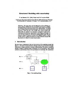
Now we are dealing with three probability spaces: SA and SB for BN1 and BN2, and SAB for P (A, B). The mapping from A to B amounts to determine the distribution of B in SB , given the distribution P (A) in SA under the constraint P (A, B) in SAB . To propagate probabilistic influence across these spaces, we can apply Jeffrey’s rule and treat the probability from the source space as soft evidence to the target space [27, 33]. This rule goes as follow. When the soft evidence on X, represented as the distribution Q(X), is presented, not only P (X), the original distribution of X, is changed to Q(X), all other variables Y will change their distributions from P (Y ) to Q(Y ) according to (8) X Q(Y ) = P (Y |Xi )Q(Xi ) (8) i

where the summation is over all states Xi of X. As depicted in Fig. 9, mapping A to B is accomplished by applying Jeffrey’s rule twice, first from SA to SAB , then SAB to SB . Since A in SA is identical to A in SAB , P (A) in SA becomes soft evidence Q(A) to SAB and by (8) the distribution of B in SAB is updated to X Q(B) = P (B|Ai )Q(Ai ) (9) i

Q(B) is then applied as soft evidence from SAB to node B in SB , updating beliefs for every other variable V in SB by P Q(V ) = P (V |Bj )Q(Bj ) j P P = P (V |Bj ) P (Bj |Ai )Q(Ai ) (10) j i P P = P (V |Bj ) P (Bj |Ai )P (Ai ) j

i

A P(A) BN1

B Soft Evidence

SAB: P(A,B) Q(A) Q(B)

Soft Evidence

Jeffrey’s rule

Q(B) BN2

Fig. 9. Mapping Concept A to B

Back to the example in Fig. 6, where the posterior distribution of “Human”, given hard evidence ¬M ale u Animal, is (T rue 0.102, F alse 0.898). Suppose we have another BN which has a variable “Adult” with marginal distribution (T rue 0.8, F alse 0.2). Suppose we also know that “Adult” is similar to “Human” with conditional distribution (“T ” for “True”, “F ” for “False”)

24

Zhongli Ding, Yun Peng, and Rong Pan

P (Adult|Human) = T F

µT 0.7 0.0

F ¶ 0.3 1.0

Mapping “Human” to “Adult” leads to a change of latter’s distribution from (T rue 0.8, F alse 0.2) to (T rue 0.0714, F alse 0.9286) by (9). This change can then be propagated to further update believes of all other variables in the target BN by (10). 4.2 Mapping Reduction A pair-wise linkage as described above provides a channel to propagate belief from A in BN1 to influence the belief of B in BN2. When the propagation is completed, (9) must hold between the distributions of A and B. If there are multiple such linkages, (9) must hold simultaneously for all pairs. In theory, any pair of variables between two BNs can be linked, albeit with different degree of similarities. Therefore we may potentially have n1 × n2 linkages ( n1 and n2 are the number of variables in BN1 and BN2, respectively). Although we can update the distribution of BN2 to satisfy all linkages by IPFP using (9) as constraints, it would be a computational formidable task.

Fig. 10. Mapping Reduction Example

Fortunately, satisfying a given probabilistic relation between P (A, B) does not require the utilization, or even the creation, of a linkage from A to B. Several probabilistic relations may be satisfied by one linkage. As shown in Fig. 10, we have variables A and B in BN1, C and D in BN2, and probability relations between every pair as below: µ ¶ µ ¶ 0.3 0.0 0.33 0.18 P (C, A) = , P (D, A) = , µ0.1 0.6 ¶ µ 0.07 0.42 ¶ 0.348 0.162 0.3 0.0 P (D, B) = , P (C, B) = . 0.112 0.378 0.16 0.54 However, we do not need to set up linkages for all these relations. As Fig. 10 depicts, when we have a linkage from A to C, all these relations are satisfied

BayesOWL: Uncertainty Modeling in Semantic Web Ontologies

25

(the other three linkages are thus redundant). This is because not only beliefs on C, but also beliefs on D are properly updated by mapping A to C. Several experiments with large BNs have shown that only a very small portions of all n1 × n2 linkages are needed in satisfying all probability constraints. This, we suspect, is due to the fact that some of these constraints can be derived from others based on the probabilistic interdependencies among variables in the two BNs. We are currently actively working on developing a set of rules that examine the BN structures and CPTs so that redundant linkages can be identified and removed.

5 Conclusion This chapter describes our on-going research on developing a probabilistic framework for modeling uncertainty in semantic web ontologies based on Bayesian networks. We have defined new OWL classes (“PriorProb”, “CondProb”, and “Variable”), which can be used to encode probability constraints for ontology classes and relations in OWL. We have also defined a set of rules for translating OWL ontology taxonomy into Bayesian network DAG and provided a new algorithm D-IPFP for efficient construction of CPTs. The translated BN is semantically consistent with the original ontology and satisfies all given probabilistic constraints. With this translation, ontology reasoning can be conducted as probabilistic inferences with potentially better, more accurate results. We are currently actively working on extending the translation to include properties, developing algorithms to support common ontology-related reasoning tasks. Encouraged by our preliminary results, we are also continuing work on ontology mapping based on BayesOWL. This includes formalizing concept mapping between two ontologies as probabilistic reasoning across two translated BN, and addressing the difficult issue of oneto-many mapping and its generalized form of many-to-many mapping where more than one concepts need to be mapped from one ontology to another at the same time. The BayesOWLframework presented in this chapter relies heavily on the availability of probabilistic information for both ontology to BN translation and ontology mapping. This information is often not available (or only partially available) from domain experts. Learning these probabilities from data then becomes the only option for many applications. Our current focus in this direction is the approach of text classification [5, 21]. The most important and also most difficult problem in this approach is to provide high quality sample documents to each ontology class. We are exploring ontology guided search of the web for such documents. Another interesting direction for future work is to deal with inconsistent probability information. For example, in constructing CPTs for the translated BN, the given constraints may be inconsistent with each other, also, a set of consistent constraints may itself be inconsistent with the network structure.

26

Zhongli Ding, Yun Peng, and Rong Pan

This issue involves detection of inconsistency, identification of sources of inconsistency, and resolution of inconsistency.

References 1. Agarwal S, Hitzler P (2005) Modeling Fuzzy Rules with Description Logics. In Proceedings of Workshop on OWL Experiences and Directions. Galway, Ireland 2. Bock HH (1989) A Conditional Iterative Proportional Fitting (CIPF) Algorithm with Applications in the Statistical Analysis of Discrete Spatial Data. Bull. ISI, Contributed papers of 47th Session in Paris, 1:141–142 3. Cooper GF (1990) The Computational Complexity of Probabilistic Inference using Bayesian Belief Network. Artificial Intelligence 42:393–405 4. Cramer E (2000) Probability Measures with Given Marginals and Conditionals: I-projections and Conditional Iterative Proportional Fitting. Statistics and Decisions, 18:311–329 5. Craven M, DiPasquo D, Freitag D, McCallum A, Mitchell T, Nigam K, Slattery S (2000) Learning to Construct Knowledge Bases from the World Wide Web. Artificial Intelligence, 118(1-2): 69–114 6. Csiszar I (1975) I-divergence Geometry of Probability Distributions and Minimization Problems. The Annuals of Probability, 3(1):146–158 7. Deming WE, Stephan FF (1940) On a Least Square Adjustment of a Sampled Frequency Table when the Expected Marginal Totals are Known. Ann. Math. Statist. 11:427–444 8. Ding Z, Peng Y (2004) A Probabilistic Extension to Ontology Language OWL. In Proceedings of the 37th Hawaii International Conference on System Sciences. Big Island, HI 9. Ding Z, Peng Y, Pan R (2004) A Bayesian Approach to Uncertainty Modeling in OWL Ontology. In Proceedings of 2004 International Conference on Advances in Intelligent Systems - Theory and Applications (AISTA2004). LuxembourgKirchberg, Luxembourg 10. Ding Z, Peng Y, Pan R, Yu Y (2005) A Bayesian Methodology towards Automatic Ontology Mapping. In Proceedings of AAAI C&O-2005 Workshop. Pittsburgh, PA, USA 11. Doan A, Madhavan J, Domingos P, Halvey A (2003) Learning to Map between Ontologies on the Semantic Web. VLDB Journal, Special Issue on the Semantic Web 12. Fukushige Y (2004) Representing Probabilistic Knowledge in the Semantic Web. Position paper for the W3C Workshop on Semantic Web for Life Sciences. Cambridge, MA, USA 13. Giugno R, Lukasiewicz T (2002) P-SHOQ(D): A Probabilistic Extension of SHOQ(D) for Probabilistic Ontologies in the Semantic Web. INFSYS Research Report 1843-02-06, Wien, Austria 14. Gruber TR (1993) A Translation Approach to Portable Ontology Specifications. Knowledge Acquisition, 5(2):199–220 15. Heinsohn J (1994) Probabilistic Description Logics. In Proceedings of UAI-94, 311–318 onen E (2004) Probabilistic Information Retrieval based on Con16. Holi M, Hyv¨ ceptual Overlap in Semantic Web Ontologies. In Proceedings of the 11th Finnish AI Conference, Web Intelligence, Vol. 2. Finnish AI Society, Finland

BayesOWL: Uncertainty Modeling in Semantic Web Ontologies

27

17. Jaeger M (1994) Probabilistic Reasoning in Terminological Logics. In Proceedings of KR-94, 305–316 18. Koller D, Levy A, Pfeffer A (1997) P-CLASSIC: A Tractable Probabilistic Description Logic. In Proceedings of AAAI-97, 390–397 19. Kruithof R (1937) Telefoonverkeersrekening. De Ingenieur 52:E15–E25 20. Lauritzen SL, Spiegelhalter DJ (1988) Local Computation with Probabilities in Graphic Structures and Their Applications in Expert Systems. J. Royal Statistical Soc. Series B 50(2):157–224 21. McCallum A, Nigam K (1998) A Comparison of Event Models for Naive Bayes Text Classification. In AAAI-98 Workshop on “Learning for Text Categorization” 22. Noy NF (2004) Semantic Integration: A Survey Of Ontology-Based Approaches. SIGMOD Record, Special Issue on Semantic Integration, 33(4) 23. Pan JZ, Stamou G, Tzouvaras V, Horrocks I (2005) f-SWRL: A Fuzzy Extension of SWRL. In Proc. of the International Conference on Artificial Neural Networks (ICANN 2005), Special Section on “Intelligent multimedia and semantics”. Warsaw, Poland 24. Pan R, Ding Z, Yu Y, Peng Y (2005) A Bayesian Network Approach to Ontology Mapping. In Proceedings of ISWC 2005. Galway, Ireland 25. Pearl J (1986) Fusion, Propagation and Structuring in Belief Networks. Artificial Intelligence 29:241–248 26. Pearl J (1988) Probabilistic Reasoning in Intelligent Systems: Networks of Plausible Inference. Morgan Kaufman, San Mateo, CA 27. Pearl J (1990) Jefferys Rule, Passage of Experience, and Neo-Bayesianism. In H.E. et al. Kyburg, Jr., editor, Knowledge Representation and Defeasible Reasoning, 245–265. Kluwer Academic Publishers 28. Peng Y, Ding Z (2005). Modifying Bayesian Networks by Probability Constraints. In the Proceedings of UAI 2005. Edinburgh, Scotland 29. Prasad S, Peng Y, Finin T (2002) A Tool For Mapping Between Two Ontologies. Poster in International Semantic Web Conference (ISWC02), Sardinia, Italy 30. van Rijsbergen CJ (1979). Information Retrieval. Lodon:Butterworths, Second Edition 31. Straccia U (2005) A Fuzzy Description Logic for the Semantic Web. In Sanchez, E., ed., Capturing Intelligence: Fuzzy Logic and the Semantic Web. Elsevier 32. Stuckenschmidt H, Visser U (2000) Semantic Translation based on Approximate Re-classification. In Proceedings of the Workshop “Semantic Approximation, Granularity and Vagueness”, KR’00 33. Valtorta M, Kim Y, Vomlel J (2002) Soft Evidential Update for Probabilistic Multiagent Systems. International Journal Approximate Reasoning 29(1): 71– 106 34. Vomlel J (1999) Methods of Probabilistic Knowledge Integration. PhD Thesis, Department of Cybernetics, Faculty of Electrical Engineering, Czech Technical University 35. Xiang Y (2002) Probabilistic Reasoning in Multiagent Systems: A Graphical Models Approach. Cambridge University Press 36. Yelland PM (1999) Market Analysis Using Combination of Bayesian Networks and Description Logics. Sun Microsystems Technical Report TR-99-78