4 Chess. 3196 2. 36. 0. 5 Contraceptive Method Choice 1473 3. 7. 2. 6 Dermatology. 366 6. 33. 1 ... 21 Thyroid ANN. 7200 3. 15. 0. 22 Tic-Tac-Toe Endgame.
Beam Search Extraction and Forgetting Strategies on Shared Ensembles⋆ V. Estruch
C. Ferri
J. Hern´andez-Orallo
M.J. Ram´ırez-Quintana
DSIC, Univ. Polit`ecnica de Val`encia , Cam´ı de Vera s/n, 46020 Val`encia, Spain. {vestruch,cferri,jorallo,mramirez}@dsic.upv.es
Abstract. Ensemble methods improve accuracy by combining the predictions of a set of different hypotheses. However, there is an important shortcoming associated with ensemble methods. Huge amounts of memory are required to store a set of multiple hypotheses. In this work we devise an ensemble method that partially solves this drawbacks. The key point is that components share their common parts. For this goal, we employ a multi-tree, a structure that can simultaneously contain an ensemble of decision trees, but with the advantage that decision trees share some conditions. To construct this multi-tree we define an algorithm based on a beam search with several extraction criteria and with several forgetting policies for the suspended nodes. Finally, we compare the behaviour of this ensemble method with some well-known methods for generating hypothesis ensembles. Keywords: Ensemble Methods, Decision Trees, Randomisation, Search Space, Beam Search, Option Trees.
1
Introduction
Ensemble methods [6] are used to improve the accuracy of machine learning models. Basically, this technique combines a finite set of hypotheses in order to get a new one, usually more accurate than any of the ensemble. Well-known ensemble methods are boosting, bagging, randomisation, etc. Although accuracy is significantly increased, a large amount of computational resources is necessary to generate, store, and employ the ensemble due to the large number of different hypotheses that must conform the ensemble. For this reason, there are several contexts where these techniques are hard to apply. Since ensemble methods construct a set of models, one way to overcome these hindrances could be to share the common parts of the models. In our framework (decision tree learning), we share the common branches of the trees. In previous works [8], we presented an algorithm which is able to obtain more than one tree. It is based on a structure, called multi-tree, which can contain a set of decision trees that have in common some of their conditions. In order to generate a multitree, once a splitting criterion is applied on a node, we store the splits which have ⋆
This work has been partially supported by CICYT under grant TIC2001-2705-C0301 and Acci´ on Integrada Hispano-Austr´ıaca HA2001-0059.
not been selected into a list of suspended nodes. The selected split is pursued until a complete tree is constructed. Later, alternative models can be generated by exploring the nodes of the list. This way of exploring the space to generate an ensemble of hypotheses can be seem as a beam search. Consequently, the use of an auxiliary data structure (list of suspended nodes) must lead to establish a policy to manage it. This policy must cover several aspects such as the definition of a criterion to extract a node in order to populate further the multi-tree. In this paper we focus on the study of some strategies of selecting the nodes to be explored from the list of suspended nodes. We will introduce some methods, and then we will study experimentally these strategies. We compare the performance of this ensemble method with other well-known methods as bagging [2] and boosting [9]. Despite the advantages of the multi-tree approach, there is a great amount of suspended nodes that are never employed. Thus, they are occupying memory needlessly and it would be interesting to try to forget these nodes. We study some techniques to keep only a subset of the nodes into consideration. This forgetting technique leads to a better use of resources as we experimentally demonstrate. The paper is organised as follows. In section 2, we introduce the multi-tree structure. Section 3 includes some experimental evaluation about multi-tree construction. It also explains different forgetting strategies and shows the results of several experiments related to this technique. Finally, section 4 closes the paper with the conclusions and future work.
2
Shared Ensembles
Ensemble methods require the generation, storage and application of a set of models in order to predict future cases. This represents an important consumption of resources, in both scenarios: learning process and predicting new cases. In previous work [8] we presented a method that allows a set of decision trees to be generated from a single evidence. A collection of trees is called a forest, but our approach is based on a shared ensemble, namely , a collection of trees that share their common parts (decision multi-tree). The decision multi-tree learning method is based on classical decision-tree learning; more precisely, the idea is to generate an AND/OR tree structure called multi-tree, from which it is possible to extract a set of hypotheses. We perform a greedy search for each solution, but once the first solution is found the following ones can be obtained taking into consideration a limited computation time. Therefore, our algorithm can be considered anytime in a certain way. An anytime algorithm is one that can be interrupted at any point during computation to return a result whose quality increases with increasing computation time [5]. Since a multi-tree can contain a set of hypotheses, we employ an ensemble method that combines the individual components of the multi-tree. This ensemble method takes profit of the internal structure of the multi-tree by sharing common parts of the components of the ensemble. In this way the amount of re2
sources required for the learning and the application of the ensemble is reduced. We called this new ensemble method: shared ensemble. A decision multi-tree structure is similar to an option tree [4, 3, 10]. The main difference between these methods is the construction strategy. In the multi-tree method, we store all the rejected splits as suspended nodes, and later we continue the multi-tree construction selecting one of these suspended nodes according to a criterion. Option trees are constructed as usual, but when at a level the difference between the best test with the other possible is small, these are also explored as optional tests (OR-nodes). The creation of optional nodes is limited at the upper levels to restrict the size of the option tree. Therefore, while options trees are constructed by a breadth search, a multi-tree is generated by following a beam search, i.e. we store the discarded alternatives in a list of suspended nodes, and later, if we want to populate further the multi-tree, we select one node from the list according to one selection criterion, and at this point the search is continued. As we have just seen in section 1, the decision multi-tree can be populated by selecting one suspended OR-node from the list of suspended OR-nodes by means of a selection criterion (suspended OR-node selection criterion).The optimality computed for the splitting criterion can be used to choose the OR-node to be explored. We have introduced the following suspended OR-node selection criteria: – Rival Absolute: From the list of suspended OR-nodes, the node with highest optimality is selected. – Rival Ratio: For every suspended OR-node, a rival ratio value is computed, as the relation between the optimality of the OR-node and the best optimality of its sibling OR-nodes (i.e. the children of the same AND-node). The suspended OR-node with highest rival ratio value is chosen. – Rival Ratio with Depth Weighted: This criterion is identical to the rival ratio criterion, but in this case we add to the split ratio value a factor that depends inversely on the depth of the OR-node. – Random: This criterion just selects nodes pseudo-randomly (uniform distribution) from the list. – Random with Depth Weighted: This criterion just selects nodes in a pseudo-random way but in this case taking into account the depth of the selected node. – TopMost: Select first the topmost node with highest optimality. Once the multi-tree construction, it contains a set of hypotheses depending on the number of suspended OR-nodes which have been explored. Note that the number of hypotheses increases exponentially w.r.t. the number of nodes explored. Since it could be prohibitive to combine all this models at top, the combination is performed inside the multi-tree structure.
3
Experiments
In this section, we present an experimental evaluation of our approach, as is implemented in the SMILES system [7]. SMILES is a multi-purpose machine 3
learning system which (among many other features) includes the implementation of a multiple decision tree learner. For the experimental evaluation, we have employed 23 datasets from the UCI dataset repository [1]. Some details of the datasets are included in Table 1. For the experiments, we used GainRatio [11] as splitting criterion. Pruning is not enabled. The experiments were performed in a Pentium III-800 Mhz with 180MB of memory running Linux 2.4.2. The results show the geometric mean of running 10 times a 10-fold cross-validation for each dataset with a different multi-tree construction. First, we analyse the behaviour of the quality of the shared ensemble depending on some criteria to populate the multi-tree: Bottom, Optimal, Random, Rival Ratio and Top Most. # 1 2 3 4 5 6 7 8 9 10 11 12 13 14 15 16 17 18 19 20 21 22 23
Datasets Balance Scale Breast Cancer Breast Cancer Wisconsin Chess Contraceptive Method Choice Dermatology Hayes-Roth Heart Disease Hepatitis Horse-colic-outcome Horse-colic-surgical House Congressional Voting Iris Plan MONK’s1 MONK’s2 MONK’s3 New Thyroid Postoperative Patient Segmentation Image Database Teaching Assistant Evaluation Thyroid ANN Tic-Tac-Toe Endgame Wine Recognition
Size 325 699 569 3196 1473 366 106 920 155 366 366 435 158 566 601 554 215 90 2310 151 7200 958 178
Classes 3 2 2 2 3 6 3 5 2 3 2 2 3 2 2 2 3 3 7 3 3 2 3
Nom. Attr. Num. Attr. 0 4 0 9 1 30 36 0 7 2 33 1 5 0 8 5 14 5 14 8 14 8 16 0 0 4 6 0 6 0 6 0 0 5 7 1 0 14 2 3 15 0 8 0 0 13
Table 1. Datasets used in the experiments.
Table 2 shows the accuracy comparison between these methods for populating the multi-tree. According to the results, the best methods to build the shared ensemble seem to be Random and Top Most. The Top Most method has an important drawback: the decision trees do not share many components, so the construction and use of the shared structure is slower. This fact is also perceived if one observes the consumption of time. Table 3 shows the average learning time for each dataset depending on the method employed to populate the multi-tree. The difference in time between Random and Top Most is important because the Top Most method selects the nodes to be explored at the top positions in the multi-tree. This leads to the generation of very different models because they do not share many conditions. However, this criterion also produces big multi-trees where the advantages in resource saving of the multi-tree structure are practically lost. Consequently, the Random criterion can be considered as an optimal trade-off between efficiency and accuracy. 4
# Bottom Optimal Random Rival Ratio Top most 1 78.18 79.00 82.61 77.63 86.60 2 93.84 94.70 94.88 93.45 94.45 3 92.43 92.55 93.07 93.75 93.75 4 99.62 99.58 99.38 99.64 99.62 5 48.35 48.23 49.73 48.31 51.70 6 91.86 92.92 94.03 92.17 91.31 7 76.44 76.75 76.75 73.06 76.75 8 52.23 52.48 54.43 52.20 59.13 9 76.07 75.87 81.40 75.93 83.67 10 62.72 62.78 67.28 62.69 75.28 11 78.53 78.00 83.36 78.33 85.83 12 94.70 95.53 95.67 94.35 95.23 13 94.13 94.13 95.33 94.20 94.67 14 95.20 95.91 99.78 99.73 100.00 15 75.42 75.33 75.67 71.05 77.55 16 98.02 98.02 97.85 97.38 97.95 17 92.14 93.38 93.29 93.14 92.43 18 64.63 63.75 63.25 69.88 63.00 19 95.91 95.91 96.40 96.06 96.06 20 60.47 60.60 62.93 60.07 63.40 21 99.24 99.37 99.26 99.23 99.19 22 77.21 76.97 82.01 78.13 84.94 23 92.94 92.59 93.06 94.00 90.00 Geomean 80.56 80.70 82.45 80.69 83.61
Table 2. Accuracy of combination depending on the second tree criterion.
Node forgetting Despite the advantages of the multi-tree structure, many suspended nodes are never ‘woken’, occupying memory needlessly. An additional criterion can be specified to forget some of the suspended nodes and, hence, to use less memory. Since we have seen that a good criterion is to select the nodes to be explored randomly, a random strategy of node forgetting will not alter the suspended node selection criterion, and therefore the accuracy of the multiclassifier will not be degraded. We have studied several methods to restrict the nodes to be selected: – Constant: We only store a constant minimum number of nodes. – Logarithmic: A logarithmic number of nodes is selected (there is a constant minimum too). – Logarithmic + depth: A logarithmic number of nodes is selected corrected by the depth of the nodes (there is a constant minimum too). This correction tends to store more nodes at the top positions, where the exploration of suspended nodes permits models to become more diverse. A comparison of some of these criteria according to the accuracy of the classifiers obtained are presented in Table 4. These criteria are: no forgetting, limiting a constant number of nodes (5) in each OR-node, leaving a logarithmic number of nodes, and finally a correction of the last method depending on the node depth. The results of Table 4 indicate that, as expected, the forgetting process does not produce significant modifications on the quality of the classifiers. Table 5 contains the average learning time for each classifier and dataset, and the geometric mean of all the datasets. The experiments demonstrate the usefulness of node forgetting, because it reduces the learning time. The best forgetting method is the one based on the selection of a logarithmic number of all possible nodes. The corrected version (log + depth) is a bit slower because it selects nodes at the top of the multi-tree. The method based on a constant 5
# Bottom Optimal Random Rival Ratio Top most 1 0.05 0.06 1.10 0.08 31.41 2 0.81 0.34 2.47 0.29 21.92 3 0.09 0.56 11.86 8.77 136.39 4 0.39 0.63 5.78 0.91 0.30 5 0.56 0.46 5.64 40.11 939.99 6 0.30 0.33 3.51 1.09 16.03 7 0.04 0.02 0.07 0.03 0.03 8 0.40 0.36 5.00 5.64 255.20 9 0.06 0.07 1.52 0.13 7.92 10 0.21 0.18 3.59 0.58 83.75 11 0.17 0.14 3.19 0.26 41.93 12 0.02 0.08 0.54 0.07 2.62 13 0.03 0.12 0.35 0.05 1.59 14 0.16 0.02 0.16 0.04 0.26 15 0.02 0.03 0.29 0.07 1.05 16 0.03 0.02 0.15 0.02 0.18 17 0.01 0.16 0.91 0.96 6.93 18 0.01 0.02 0.21 0.03 0.49 19 1.32 2.71 15.92 28.78 15.82 20 0.03 0.04 0.85 11.40 118.58 21 1.24 2.17 11.31 7.56 14.62 22 0.05 0.05 0.46 0.06 9.02 23 0.06 0.57 1.99 0.68 880.00 Geomean 0.10 0.14 1.34 0.46 9.12
Table 3. Average learning time (in seconds) depending on the second tree criterion.
number also improves the learning time, however the results in accuracy are a bit worse than the logarithmic method. Regarding the improvement of memory, Table 6 shows the memory (in Kilobytes) required by the system to learn the multi-trees for some datasets. We also include the percentage of memory employed by the forgetting method with respect to the original method (no forgetting). For big and medium problems the use of forgetting reduces drastically the use of memory. However, for small problems the reduction is more limited. The forgetting method that requires less memory is “logarithmic”. According to these experiments, the best suspended-node forgetting criterion seems to be randomly leaving a logarithmic number of nodes, without taking depth into account. 3.1
Comparison with other ensemble methods
Let us compare the behaviour of the shared ensemble technique using forgetting with other popular ensemble methods: Bagging and Boosting (Adaboost). We have employed the Weka (version 3.2.3)1 implementation of these two ensemble methods. The ensemble methods use J48 as base classifier (the Weka version of C4.5), and we have used the default settings. Pruning is only enabled for Boosting, since this method requires pruning to get good results. Figure 1 shows the average accuracy obtained by the three methods depending on the number of the iterations. Initially, the best results are obtained by Boosting, whereasBagging and Multi-tree stay slightly lower. This is most probably because they do not use pruning. When the number of iterations of the 1
http://www.cs.waikato.ac.nz/∼ml/weka/
6
# No forgetting Const=5 Logarithmic Log. + depth 1 82.61 81.40 82.24 85.11 2 94.88 95.16 94.93 94.81 3 93.07 93.36 93.41 93.80 4 99.38 99.39 99.37 99.34 5 49.73 49.30 49.51 52.65 6 94.03 94.53 94.42 94.39 7 76.75 76.75 76.44 75.94 8 54.43 54.09 54.26 55.58 9 81.40 81.53 80.67 81.67 10 67.28 66.00 67.42 67.06 11 83.36 83.36 83.19 83.67 12 95.67 95.86 95.91 95.79 13 95.33 95.07 95.00 95.13 14 99.78 99.78 99.89 97.56 15 75.67 75.67 76.38 71.50 16 97.85 97.85 97.75 97.67 17 93.29 93.29 93.57 92.29 18 63.25 62.00 61.88 62.13 19 96.40 96.31 96.61 96.43 20 62.93 62.40 62.87 63.40 21 99.26 99.28 99.33 99.24 22 82.01 82.22 81.78 83.96 23 93.06 92.88 93.76 92.76 GeoMean 82.45 82.22 82.38 82.55
Table 4. Accuracy of the combination in the multi-tree depending on the forgetting method.
# No forgetting Const=5 Logarithmic Log + depth 1 1.10 0.60 0.62 1.71 2 2.47 1.62 1.66 2.82 3 11.86 12.47 12.00 15.20 4 5.78 5.68 4.77 9.97 5 5.64 3.74 2.48 12.49 6 3.51 3.36 3.10 4.02 7 0.07 0.07 0.02 0.01 8 5.00 2.66 2.64 5.54 9 1.52 1.38 1.36 1.87 10 3.59 2.34 2.45 3.70 11 3.19 2.33 2.28 3.58 12 0.54 0.51 0.47 0.94 13 6.10 6.66 4.62 10.46 14 0.16 0.17 0.14 0.04 15 0.29 0.30 0.29 0.08 16 0.15 0.16 0.12 0.03 17 12.26 18.81 9.96 11.09 18 0.21 0.18 0.16 0.08 19 15.92 17.34 16.17 17.44 20 0.85 0.63 0.57 1.28 21 11.31 12.14 9.79 15.36 22 0.46 0.44 0.37 0.55 23 1.99 2.06 1.70 2.05 Geomean 1.70 1.52 1.25 1.54
Table 5. Average learning time for the combined solution in the multi-tree depending on the forgetting method.
7
# 5 19 28
Original 49512.00 4880.00 18800.00
Const=5 % Logarithmic % Log + depth % 10892.00 22.0%0 6388.00 12.90% 8328.00 16.82% 4820.00 98.77% 1484.00 30.41% 3472.00 71.15% 3268.00 17.38% 2272.00 12.09% 2608.00 13.87%
Table 6. Average memory (in Kbytes) for the combined solution in the multi-tree depending on the forgetting method.
Accuracy 82.5 82.25 82
% Accuracy
81.75 81.5 Boosting
81.25
Bagging
81
Multitree
80.75 80.5 80.25 80 79.75 1
20
40
60
80
100
Iterations
Fig. 1. Accuracy obtained by the ensemble methods depending on the number of iterations.
ensemble methods is increased, all methods improve the accuracy as expected. In this case, we can see that multi-tree is the method that further enhances the results, it even overpasses Boosting with more than 80 iterations. Note that the accuracy of Bagging with 100 classifiers is not in the figure, the cause of this absence is that the computer ran out of memory for such configuration. Finally, although the shared ensemble method has suitable properties in the accuracy of the combined classifier, the most attractive feature of this algorithm is the sharing of some parts of the members of the ensemble. This fact permits a good dealing of computational resources. Figure 2 shows the average training time of Bagging, Boosting, and Multi-tree (shared ensemble) depending on the size of the ensemble. While Bagging and Boosting2 present a linear increase of time, for the shared ensemble technique it is sub-linear. Note that the implementation features of the methods (Weka is implemented in Java, while Smiles is implemented in C++) clearly affect the training time, however this does not produce significant changes in the asymptotic behaviour of the algorithms when varying the number of iterations. 2
The observed non-liner behaviour of Boosting is due to a technique implemented in Boosting that stops the algorithm when accuracy does not improves further from iteration to iteration.
8
Training Time 3.25 3 2.75 2.5
Seconds
2.25 2 Boosting
1.75
Bagging
1.5
Multi− tree
1.25 1 0.75 0.5 0.25 0 1
20
40
60
80
100
Iterations
Fig. 2. Training time required by the ensemble methods depending on the number of iterations.
4
Conclusions
This work has presented a novel ensemble method. The main feature of this technique is the use of a structure called multi-tree that permits sharing common parts of the single components of the ensemble. For this reason, we call it shared ensemble. We have introduced some criteria to populate the multi-tree. These criteria are variations of a beam search over the multi-tree structure. We have implemented this algorithm and an experimental evaluation has been performed in order to analyse the performance of these criteria. We have also studied an optimisation that permits a better use of resources based on a selection of the nodes to be stored. Lastly, we have included a comparison of the ensemble method with some well-known ensemble methods, namely Boosting and Bagging. Due to the sharing of the common parts, much less time is required than with classical ensemble approaches to perform the same number of iterations, thus our system is very appropriate for complex problems where other ensemble methods such as Boosting or Bagging require huge amounts of memory and time. As future work, we propose the study of a new strategy for generating trees. This strategy would be different from the current random technique we have employed to explore OR-nodes, and would probably be based on the semantic discrepancy of classifiers. This technique would provide a way to improve the results of our ensemble method with fewer iterations. 9
References 1. C.L. Blake and C.J. Merz. UCI repository of machine learning databases, 1998. 2. L. Breiman. Bagging predictors. Machine Learning, 24(2):123–140, 1996. 3. W. Buntine. Learning classification trees. In D. J. Hand, editor, Artificial Intelligence frontiers in statistics, pages 182–201. Chapman & Hall,London, 1993. 4. W. L. Buntine. A Theory of Learning Classification Rules. PhD thesis, School of Computing Science in the University of Technology, Sydney, February 1990. 5. T. Dean and M. Boddy. An analysis of time-dependent planning. In Proc. of the 7th National Conference on Artificial Intelligence, pages 49–54, 1988. 6. T. G Dietterich. Ensemble methods in machine learning. In First International Workshop on Multiple Classifier Systems, pages 1–15, 2000. 7. V. Estruch, C. Ferri, J. Hern´ andez, and M. J. Ram´ırez. SMILES: A multi-purpose learning system. In Logics in Artificial Intelligence, European Conference, JELIA, volume 2424 of Lecture Notes in Computer Science, pages 529–532, 2002. 8. V. Estruch, C. Ferri, J. Hern´ andez, and M.J. Ram´ırez. Shared Ensembles using Multi-trees. In the 8th Iberoamerican Conference on Artificial. Intelligence, Iberamia’02, volume 2527 of Lecture Notes in Computer Science, pages 204–213, 2002. 9. Y. Freund and R.E. Schapire. Experiments with a new boosting algorithm. In Proc. 13th International Conference on Machine Learning, pages 148–146. Morgan Kaufmann, 1996. 10. R. Kohavi and C. Kunz. Option decision trees with majority votes. In Proc. 14th International Conference on Machine Learning, pages 161–169. Morgan Kaufmann, 1997. 11. J. R. Quinlan. C4.5: Programs for Machine Learning. Morgan Kaufmann, San Mateo, CA, 1993.
10