order to recursively spawn new beams that in turn may be reflected, transmitted ... diffraction beam spans the area between the shadow boundary of the parent ...
Beam Tracing for Multipath Propagation in Urban Environments Arne Schmitz∗ , Tobias Rick+ , Thomas Karolski∗ , Leif Kobbelt∗ , Thorsten Kuhlen+ ∗
Computer Graphics Group, + Virtual Reality Group, RWTH Aachen University
Abstract— We present a novel method for efficient computation of complex channel characteristics due to multipath effects in urban microcell environments. Significant speedups are obtained compared to state-of-the-art ray-tracing algorithms by tracing continuous beams and by using parallelization techniques. We optimize simulation parameters using on-site measurements from real world networks.
data had to be transformed into images and algorithms had to be turned into image synthesis. Today, graphics hardware can be programmed by an extension of the C programming language. This has the great advantage that the computational power can be accessed even by non-graphics experts.
I. I NTRODUCTION
The theoretical foundation of radio wave propagation can be found in [1] whereas [2] gives a more recent overview on radio propagation models and algorithms. In literaure, it is very common to distinguish between stochastic (empirical) channel models and deterministic propagation algorithms. Well-known examples of empirical models are the work of Hata [3] and Ikegami [4]. They propose to model the radio propagation phenomena by approximating the actual propagation loss (path loss) by parametrized functions. Hata determined the values of the parameters by conducting extensive measurement campaigns. Ikegami extended Hata’s work by analyzing the dependence of approximate equations with respect to height gain, street width, propagation distance and radio frequency. Such empirical models are typically characterized by short evaluation time but are prone to huge prediction errors and perform especially poor in heterogeneous propagation environments like historically grown cities [5]. Therefore, most deterministic algorithms for predicting radio signal strength rely on the computation of actual propagation paths due to wave guiding effects like reflection, diffraction and scattering. Classical ray tracing was introduced by Whitted [6] for image synthesis. Since then it has been successfully applied and extended in numerous publications in order to compute global illumination effects based on geometrical optics. Global illumination and radio wave propagation are essentially the same problem statement, although they differ slightly in the kind of optical effects that are simulated. Diffraction and interference for example are usually left out of global illumination, due to the subtlety of the effect. In [7] Ikegami showed that ray tracing is also an excellent technique for estimating radio propagation losses. Based on ray tracing algorithms, Schaubach [8], Schmitz [9] and Kim [10] state that their predicted path loss values were generally within 4 to 8 dB of the measured path loss. Such predictions are considered to be of very high accuracy. However, high computation times still prevent the application of ray tracing algorithms in large scale network analysis, such as network planning and optimization.
The formulation of exact models for propagation losses is a typical task in the planning of mobile communication systems. Two main strategies can be identified. First, an empirical formulation of the propagation losses can be applied. Second, deterministic approaches, like the theory of diffraction, evaluate actual propagation paths due to complex interaction of radio waves with the environment. The latter usually relies on ray tracing techniques. One great advantage of deterministic models is the high accuracy in the spatial domain of simulation scenarios. Although empirical models produce good results on average, they are prone to significant errors where deterministic effects like reflection or diffraction are predominant since they tend to ignore visibility information. However, the design and planning of future communication systems requires a detailed analysis of additional channel characteristics besides propagation losses, like the delay and angular spread of the arriving signals. The computation of such characteristics requires a deterministic model like ray tracing, which is computationally expensive. Therefore, we consider the reduction of computation time to be an important research challenge which we want to address in this paper. The second contribution is a scheme for optimizing simulation parameters from real world measurements. Ray tracing algorithms are well studied and are known to achieve very high accuracy, but at the cost of long computation times. Computing the path loss for an urban scenario can take minutes to hours, depending on accuracy and the number of considered effects. However, the computations are independent of each other, allowing for parallelization of the tasks. Today, the most economic parallelization can be implemented on graphics cards, which feature multi-core processors that allow to run parallelized problems with hundreds of threads. Current GPUs achieve over 1000 GFLOPs compared to recent quadcore CPUs which achieve only around 50 GFLOPs. Until recently, the main challenge of utilizing graphics hardware for scientific computations was to map general algorithms to fit in the graphics computation pipeline. Input
II. R ELATED W ORK
The idea of ray tracing can be extended to the concept of beams, which are a continuum of rays. Beam tracing was introduced by Heckbert and Hanrahan [11]. It reduces intersection tests, as well as overcomes sampling problems, since ray samples tend to become too sparse or too dense. Many more works have been published in this area, which also concentrated on realtime rendering [12], or non-graphical applications such as audio rendering [13]. However, our approach takes the beam tracing idea to a different level of applications, not simulating light, but the radiation of different radio frequency bands. In combination with our novel data structures and an efficient implementation using general purpose GPU programming, this allows us to calculate field attenuation and delay spread at the same time with high accuracy and in a speed not possible before. Similar to our approach is the work by Rajkumar et al. [14], who also used a form of beam tracing for wave propagation, but determines visibility differently. Furthermore, Rick et.al. presented an GPU-based approach to radio wave propagation in Catrein [15] and Rick [16]. They trace propagation paths in a discrete fashion by repeated rasterization of line-of-sight regions. By restricting computations to the strongest path only, propagation predictions are delivered at interactive rates. However, since only the mean received signal strength is computed, multipath effects, which are an essential requirement for delay spread estimations, are completely neglected. This is not the case with our algorithm. Besides basic propagation losses, advanced channel characteristics like the delay spread are computed at a considerably reduced run time. III. OVERVIEW In general, our algorithm is an outdoor prediction method for microcell urban environments. The computation will require a building database of the area in question. We target common mobile communication frequencies ranging from 900 MHz up to a few GHz. We present a novel method for the efficient computation of complex channel characteristics by combining concepts of both electromagnetic principles and computer graphics. A significant speedup in computation time is achieved by a twofold strategy. First, we replace the tracing of single rays by a tracing of full beams. And second, we parallelize our implementation on a many-core architecture, namely on graphics hardware using the NVIDIA CUDA compute platform. This leads to the following benefits. Since a wide beam covers more ground than a single ray, fewer beams than rays have to be traced. Additionally, the use of beams circumvents the problem of low spatial resolution in receiver space, an issue which is often encountered in classical ray tracing algorithms when too few rays are launched. Using many processing cores leads to an extremely efficient beam-geometry intersection. Multiple objects are intersected with the same beam at the same time. Overall, the computation of an urban scenario with one transmitter takes place in mere seconds, including all described effects. This is an order of magnitude faster than previous ray-tracing approaches.
Fig. 1. A beam is defined by four edges. The two edges e1 and e2 form a quadrilateral whose baseline i we call the image plane of the beam. The point o is the (virtual) origin of the beam. A ray r = o + λd is constructed through the image plane and intersected with the face {f1 , f2 } which was identified in the beam framebuffer.
The calculation of propagation losses can be divided into two parts, a geometric computation and subsequent application of electromagnetic principles. In the first geometric step, our algorithm finds multiple paths up to a certain number of interactions. These types of interaction consist of typical propagation phenomena like free space propagation, diffraction and reflection. When all relevant ray paths have been identified common techniques from electromagnetics, e.g., GTD or UTD, can be applied to compute signal strength, phase and delay for each ray contained in a beam. Unknown components (like traffic or vegetation) of the propagation environment is modeled by introducing correction factors to our path loss model which can be adapted by site-specific measurements. We consider one of the main applications to be in the area of automatic network planning for future mobile communication systems where additional channel characteristics like delay spread are essential for finding optimal antenna locations and configurations. IV. A LGORITHM Our approach allows to rapidly and accurately compute two important aspects of radio wave propagation: the field strength and a delay spread histogram at arbitrary points in the scene. The underlying algorithm consists of two parts. Building a beam hierarchy that describes the propagation of the electromagnetic radiation, and the evaluation of radio field properties based on this beam hierarchy. The tracing algorithm relies on a small rendering pipeline similar to OpenGL, but implemented in CUDA, to determine the split positions inside of each beam. For efficiency, unnecessary geometry is clipped away by the use of a quadtree that is intersected with the beam. The pseudo code of the tracing algorithm is as follows: 1. Build scene geometry quadtree 2. Trace initial beams from source 1 Clip geometry to beam using quadtree 2 Split beam according to visible geometry 3 Generate reflected, refracted and diffracted beams 4 Update signal time and attenuation for beam 5 Trace recursively
(a)
(a)
(b)
(c)
(d)
Fig. 2. (a) A beam is created and intersected with the geometry. (b) The beam is split into child-beams, according to the intersections. (c) Reflection edges are identified, and the old beam origin is reflected at those edges, constructing reflected beams. (d) In the same manner diffraction beams are generated at silhouette edges.
The evaluation of the generated beams also uses a simplified rasterization pipeline, which accumulates the beam attenuation and the delay into 2D and 3D framebuffers. The pseudo code of the evaluation algorithm is thus: 1. Iterate over all beams 1 Rasterize beam attenuation into 2D array 2 Rasterize beam delay into 3D histogram
(b)
(c)
Fig. 3. (a) The beam hierarchy is traversed and each beam is sampled in (b) a 2D buffer which gives rise to the path loss prediction map, and (c) the 3D delay spread histogram, which gives a delay spread plot for each point in the scene.
A. Beam Tracing A beam in 2D is defined as a quad. It represents a bundle of rays emanating from an edge, which might be degenerate in the case of a point radiation source, in which case the beam is equivalent to a triangle. Each beam carries information about signal travel time, for later evaluation of the path loss and delay spread. Our algorithm recursively generates a beam hierarchy by emanating beams at a radiation source. When a beam is formed, it has to be intersected with the scene geometry in order to recursively spawn new beams that in turn may be reflected, transmitted or diffracted at surface boundaries. A beam might be infinite at one end, if it does not intersect any geometry at all, or it might be finite, if it intersects the geometry of the scene. The splitting of a beam into new sub-beams is accomplished by simply rendering the geometry contained in the beam into a slice of a 2D buffer such that colors correspond to IDs for the geometric faces. An associated buffer stores depth information. When the faces that are hit have been identified, the exact intersection points on the surfaces are computed based on the beam origin and rasterized intersection points as illustrated in Fig. 1. The construction of sub-beams is depicted in Fig. 2. A reflected beam is constructed by simply mirroring the beam origin at the wall that the old beam has hit. Diffraction beams are constructed at silhouette edges of the geometry for every parent beam that has been split at one such edge. The diffraction beam spans the area between the shadow boundary of the parent beam and the backfacing part of the silhouette. B. Beam Evaluation In radio wave propagation, usually the path loss is computed, which is the attenuation of the signal. The most simple model for this is the freespace model, which expresses the
path loss in dB: Lfp = 10n log10 d + C
(1)
For the path loss exponent n = 2 and the system loss constant C = 0 we get the same attenuation (Φ ∼ d12 ), that is known from global illumination for the attenuation of the flux density with the distance to the light source. Given the set B of all beams of the beam tree that lead to an individual beam b, we compute the path loss Lp (x) of a point x ∈ b. We accumulate deflection loss functions fr along the way and also take the length of the propagation path x−to into account. Hence, the path loss is then defined as: Q fri (2) Lp (x) = bi ∈B 2 |x − to | The delay spread is also computed by traversing the beam tree. Here we use a 3D array for collecting the delays. Every column in this array represents a discrete delay spread histogram for the corresponding position. When we evaluate (i.e. rasterize) a beam, we compute the distance the signal has traveled. This can be mapped to a traveling time. This is then mapped to one of the bins of the histogram and the path loss is added to that bin. Accumulating over all beams gives an accurate estimation of the delay spread at this specific point of the scene. The concept is illustrated in Fig. 3 V. M ODEL PARAMETER A DAPTION It is quite common in literature to adapt propagation models to different types of environments. Instead of a qualitative description of propagation environments like rural or urban or by building density we use an implicit description by adapting model parameters to different environments by calibration from real-world measurements. Thus, we model unknown components, like traffic or vegetation, of the propagation
environment by introducing variable coefficients (model parameters) into our path loss calculation. We formulate the adaption of model parameters as a constrained least-squares problem: x
x
X
Fi2 (x)
(3)
9 8,5 8
Time [s]
2
min ||F (x)||2 = min
9,5
7,5
i
7
such that
6,5
(4)
A·x ≤ b
(5)
B·x = c
(6)
Each row of the matrix C corresponds to one measurement location, whereas the columns are formed by the beams that reach the respective location, like travel distance of each arriving path and number of reflections and diffractions. This can be done, since we choose to optimize the logarithm of the path loss formula (2) and thus the product in the nominator is transformed to a sum which can be expressed easily in matrix notation. The vector d contains the measured path loss at each location, hence the optimal parameter vector x ˆ minimizes the mean squared error between the predicted and measured path loss with respect to the constraints (5) and additionally satisfying the equality constraints (6). The constraints can be derived by expert knowledge on the propagation phenomena. The optimal x ˆ can then be calculated by common solver algorithms like Gauss-Newton or Levenberg-Marquardt [17]. We have calculated the optimal parameter vectors for the widely known Munich dataset from the COST 231 project which contains a 3D model of Munich downtown and three measurement routes. Fig. 6 shows the shape of the optimal parameter vectors for each measurement path, separately. Although, the curves differ slightly in scale, they agree on the overall shape. The standard deviation between the optimal parameter vectors of route 1 and route 2 respectively, lie between 3 and 4 when compared to the optimal parameters of route 3. Therefore, we haven chosen the parameter vector of the third measurement route for the actual computation of path loss.
0
16
32
48
64
80
96
112
128
144
160
176
X Blocksize [threads]
Fig. 4. Performance depending of grid dimensions, measured in number of threads, for four recursive reflections and diffractions. 12 10 8 6
Time [s]
= C ·x−d
4 2 0 1
2
3
4
5
6
7
Interactions
8 Diffractions Reflections
9
Fig. 5. Performance of our algorithm for varying levels of interactions. Computation complexity grows approximately linearly in the number of reflections. Optimal Parameters for all Measurement Routes Route 1 Route 2 Route 3
40
30
Parameter Value
F (x)
20
10
0
-10
VI. E VALUATION In this section we will take a look at the two most important properties of our algorithm. First we analyze the computational complexity, and second we evaluate the accuracy, compared to real-world measurements and other works. The performance of the algorithm depends of course heavily on the scene complexity which influences the beam splitting algorithm. Visibility computations are done entirely on the GPU, since it takes up the most time in our algorithm. Here, an important aspect is to find out the optimum number of concurrent threads for the chosen parallel platform. Figure 4 shows the execution time for an increasing number of parallel threads, which led to a blocksize of 128 threads executing the rasterization process in parallel.
-20 0
5
10
15
20
Parameter Index
Fig. 6.
Optimal parameter vectors for each measurement route.
However, the number of recursive reflection and diffraction steps also influences the complexity of the algorithm. In the worst case, the number of beams grow exponentially, since with every split and reflection, it will spawn a number of additional beams. However, Fig. 5 shows that with the growing number of recursive reflections, the computation time grows roughly linearly. Although each recursively created beam could lead to an exponential growth, the fact that reflected
TABLE I C OMPARISON OF OUR METHOD TO SEVERAL OTHER STATE OF THE ART WORKS . O UR METHOD SUPPORTS ALL IMPORTANT PROPAGATION EFFECTS , AND IS APART FROM THE WORK OF S CHMITZ [9], THE ONLY METHOD WHICH SIMULATES THE DELAY SPREAD . Method Our method Woelfle [18] Rick [16] Schmitz [9]
Accuracy 5m 10 m 5m 5m
Time 1.8 s 36 s 0.05 s 9m 20s
Std. dev. 6.7 dB 6.41 dB 4.5 dB 5.82 dB
mean error [dB]: 2.3 mean squared error [dB]: 7.1 std. dev. [dB]: 6.7 Prediction Measurement
80
path loss [dB]
100
120
140
160
180
0
50
100
150
200
250
300
measurement location number
Fig. 7.
Comparison between measured and predicted path loss.
beams get usually thinner limits the number of split beams created, so that in the end only one new reflected beam is created for every split beam. In the COST 231 Munich scenario there are approximately 80.000 vertices for the buildings. This is a reasonably complex scene, which is computed in several minutes on normal ray tracers for radio wave propagation. Our algorithm computes the scene in less than 2 seconds, even with complex recursive interactions. The machine used in this case was a Core2Duo with 2.4 GHz and a NVIDIA GeForce 8800 Ultra. In Fig. 7 we show a comparison between prediction and a measurement. The overall shape of the curves match, which indicates thats effects based on the scene geometry and its interaction with the radio waves are matched well by our algorithm. In Table I we compare our method to three other state of the art works. Besides timings and accuracy it is also important to compare the available features of the different algorithms. VII. C ONTRIBUTION & C ONCLUSIONS The main contribution is a novel method for the efficient computation of complex channel characteristics in a speed not possible before. Our algorithm includes important effects like multi-path propagation due to reflection and diffractions and predicts the resulting delay spread histogram. The short computation time of our algorithm will enable the large scale simulation of detailed channel models for future communication systems.
Delay spread Yes No No Yes
Reflections Yes Yes No Yes
Diffractions Yes Yes Yes Yes
R EFERENCES [1] T. S. Rappaport, Wireless Communications: Principles and Practice. Prentice-Hall, Inc., 1995. [2] L. M. Correia, Ed., COST Action 273: Mobile Broadband Multimedia Networks, Final Report. Academic Press, 2006. [3] M. Hata, “Empirical formula for propagation loss in land mobile radio services,” IEEE Trans. Veh. Technol., vol. 29, pp. 317–325, 1980. [4] F. Ikegami, S. Yoshida, T. Takeuchi, and M. Umehira, “Propagation factors controlling mean field strength on urban streets,” IEEE Trans. Antennas Propagat., vol. 32, pp. 822–829, 1984. [5] E. Damosso, Ed., COST Action 231: Digital mobile radio towards future generation systems, Final Report. Luxembourg: Office for Official Publications of the European Communities, 1999. [6] T. Whitted, “An improved illumination model for shaded display,” Commun. ACM, vol. 23, no. 6, pp. 343–349, 1980. [7] F. Ikegami, T. Takeuchi, and S. Yoshida, “Theoretical prediction of mean field strength for urban mobile radio,” IEEE Trans. Antennas Propagat., vol. 39, pp. 299–302, 1991. [8] K. R. Schaubach, N. J. D. IV, and T. S. Rappaport, “A ray tracing method for predicting path loss and delay spread in microcellular environments,” in Proc. IEEE Vehicular Technology Conference, vol. 2, May 1992, pp. 932–935. [9] A. Schmitz and L. Kobbelt, “Wave propagation using the photon path map,” in PE-WASUN ’06. New York, NY, USA: ACM, 2006, pp. 158–161. [10] S.-C. Kim, B. J. Guarino, T. M. W. III, V. Erceg, S. J. Fortune, R. A. Valenzuela, L. W. Thomas, J. Ling, and J. D. Moore, “Radio propagation measurements and prediction using three-dimensional ray tracing in urban environments at 908 mhz and 1.9 ghz,” IEEE Trans. Veh. Technol., vol. 48, pp. 931–946, 1999. [11] P. S. Heckbert and P. Hanrahan, “Beam tracing polygonal objects,” in SIGGRAPH ’84: Proceedings of the 11th annual conference on Computer graphics and interactive techniques. New York, NY, USA: ACM, 1984, pp. 119–127. [12] R. Overback, R. Ramamoorthi, and W. R. Mark, “A real-time beam tracer with application to exact soft shadows,” in EGSR, 2007. [13] T. Funkhouser, P. Min, and I. Carlbom, “Real-time acoustic modeling for distributed virtual environments,” in SIGGRAPH ’99: Proceedings of the 26th annual conference on Computer graphics and interactive techniques. New York, NY, USA: ACM Press/Addison-Wesley Publishing Co., 1999, pp. 365–374. [14] A. Rajkumar, B. F. Naylor, F. Feisullin, and L. Rogers, “Predicting rf coverage in large environments using ray-beam tracing and partitioning tree represented geometry,” Wirel. Netw., vol. 2, no. 2, pp. 143–154, 1996. [15] D. Catrein, M. Reyer, and T. Rick, “Accelerating radio wave propagation predictions by implementation on graphics hardware,” in Proc. IEEE Vehicular Technology Conference, Dublin, Ireland, 2007, pp. 510–514. [16] T. Rick and R. Mathar, “Fast edge-diffraction-based radio wave propagation model for graphics hardware,” in Proc. IEEE 2nd International ITG Conference on Antennas, Munich, Germany, March 2007, pp. 15–19. [17] K. Levenberg, “A method for the solution of certain problems in least squares,” Appl. Math., vol. 2, pp. 164–168, 1944. [18] R. Wahl, G. Wlfle, P. Wertz, P. Wildbolz, and F. Landstorfer, “Dominant path prediction model for urban scenarios,” 14th IST Mobile and Wireless Communications Summit, Dresden (Germany), 2005.