former (MVAB) creates such filters using a sam- ple covariance estimate; however, the quality of this estimate deteriorates when the sources are correlated or the ...
Beamforming using the Relevance Vector Machine
David Wipf Srikantan Nagarajan Biomagnetic Imaging Lab, University of California, San Francisco, CA 94143 USA
Beamformers are spatial filters that pass source signals in particular focused locations while suppressing interference from elsewhere. The widely-used minimum variance adaptive beamformer (MVAB) creates such filters using a sample covariance estimate; however, the quality of this estimate deteriorates when the sources are correlated or the number of samples n is small. Herein, a modified beamformer is derived that replaces this problematic sample covariance with a robust maximum likelihood estimate obtained using the relevance vector machine (RVM), a Bayesian method for learning sparse models from possibly overcomplete feature sets. We prove that this substitution has the natural ability to remove the undesirable effects of correlations or limited data. When n becomes large and assuming uncorrelated sources, this method reduces to the exact MVAB. Simulations using direction-of-arrival data support these conclusions. Additionally, RVMs can potentially enhance a variety of traditional signal processing methods that rely on robust sample covariance estimates.
1. Introduction Beamformers can be utilized to solve a general class of nonlinear estimation problems frequently encountered in signal and image processing. Suppose for a given time t we are confronted with the generative model ds X
sk (t)f (θk ) + �(t),
SRI @ MRSC . UCSF. EDU
tor, each θk ∈ Θ is a time-invariant set of parameters (where at this point Θ is unspecified), f : Θ → Cdy is a known nonlinear function, and �(t) is noise.1 Given y(t) collected over n time points, the goal here is to learn s(t)|t=1,...,n , and θk |k=1,...,ds . A surprisingly large number of parameter estimation tasks, including many maximum likelihood (ML) problems, can be expressed in this form. We will refer to this estimation problem as source localization, since often each θk corresponds with a location in Θ-space of some source (or signal) activity of interest. The associated coefficient sk (t) is then interpreted as the temporally varying source amplitude and f (·) is a mapping from a unit source at some θk to the observed data, presumably obtained using some sensor array. Note also that ds may be unknown.
Abstract
y(t) =
DAVID . WIPF @ MRSC . UCSF. EDU
(1)
k=1
where y(t) ∈ Cdy represents dy observation points, s(t) = T [s1 (t), . . . , sds (t)] ∈ Cds is an unknown coefficient vecAppearing in Proceedings of the 24 th International Conference on Machine Learning, Corvallis, OR, 2007. Copyright 2007 by the author(s)/owner(s).
Assuming that f (·) is highly nonlinear and ds is large, then estimation of each s(t) and θk can be intractable. Beamformers represent one possible solution to this problem by learning a series of spatial filters, each tailored to different values of the location parameter sampled over a fine grid in Θ-space. The observed data is then applied to each filter, and if significant energy is passed through, we assume that the associated location in Θ-space contains a source and the filtered signal corresponds to sk (t). While a wide variety of beamformers exist for this task, here we will focus on a particular variant, called the minimum variance adaptive beamformer (MVAB), that has gained widespread popularity (Van Veen et al., 1997). While simple to compute, the quality of the MVAB spatial filters is highly dependent on the number of samples n and temporal correlations present between the unknown sources, with high correlations impling a significant degradation in performance (Sekihara et al., 2002; Zoltowski, 1988). A variety of applications involve, either implicitly or explicitly, locating sources that are highly dependent or for which reliable data can be difficult to obtain. Examples include direction-of-arrival (DOA) estimation for sonar/radar applications, where Θ represents the possible angular directions of signal waves impinging upon a sensor array 1 For generality, we consider complex-valued data; however, for many applications only real-valued quantities are required.
Beamforming using the Relevance Vector Machine
(Manolakis et al., 2000; Van Veen & Buckley, 1988), and neuroelectromagnetic source imaging (Baillet et al., 2001; Van Veen et al., 1997), where Θ denotes the 3D space of voxels within the brain where significant electrical activity could potentially exist. Hence it would be very desirable to somehow adjust the MVAB to mitigate the effects of source correlations leading to more accurate spatial filtering. The relevance vector machine (RVM) (Tipping, 2001a) offers one very promising solution. Originally derived in the context of regression and classification, in this paper we will quantify how the RVM produces a data covariance estimate that is particularly useful in the context of beamforming. In the next section we will introduce the MVAB in more detail along with some of its attendant weaknesses. Section 3 will present a slightly more general version of RVMs suitable for the task at hand and discuss its role in robust covariance estimation. Section 4 then derives several analytical properties of the RVM covariance estimate that justify its use in handling source correlations. In particular, we show that in certain cases the RVM produces a modified beamformer with all source correlations completely removed. In the limit as n becomes large and assuming uncorrelated sources, this method reduces to the exact MVAB. Finally, empirical results showing the performance improvement possible using RVMs are contained in Section 5 while a brief conclusion and a discussion of related methods follows in Section 6.
the beamformer will provide using
2. Minimum Variance Adaptive Beamformer
where
The basic premise behind beamforming is to scan through Θ-space with location-dependent spatial filters, wi ∈ Cdy for sample location θi , that are sensitive to signals focused near the respective θi but filter out energy originating from elsewhere. Specifically, this implies that wiH y(t) should have a large value if θi is near to some θk from the generative model (1) and a small value everywhere else.2 Implicitly, the beamformer can be viewed as operating under the alternative (approximate) generative model y(t) =
dx X
xi (t)φi + �(t) = Φx(t) + �(t),
(2)
i=1
where Φ , [φ1 , . . . , φdx ], φi , f (θi ), x(t) , [x1 (t), . . . , xdx (t)]T , and each xi (t) is the (possibly complex) amplitude of a hypothetical latent source at location θi (the relationship between x(t) and s(t) will be clarified shortly). The θi ’s represent sampling points in Θ-space that hopefully pass near each θk . Note that the source locations have been removed as explicit parameters to estimate; rather, the value of each θk can be inferred by examining which latent sources xi (t) have substantial (nonˆ zero) power as determined by the estimate of x(t), which 2
(·)H denotes the conjugate or Hermitian transpose.
x ˆi (t) = wiH y(t), ∀i.
(3)
The corresponding basis function φi will then reflect the source location up to any quantization error. Likewise, ˆ should reflect the values of each nonzero amplitudes in x(t) sk (t). So to clarify, x(t) represents source amplitudes over a fixed sampling grid in Θ-space, most entries of which are zero-valued, while s(t) denotes only the source amplitudes at active (nonzero) locations. The number of sample points dx is assumed to be sufficiently high such that some desired resolution can be obtained, but generally we assume that dx � dy > ds . Additionally, we will treat ds as the number of nonzero xi (t) values in the generative model (2). Different beamformers are distinguished by the choice of ˆ filters wi and therefore the x(t) that results. Ideally, we would like these filters to pass exactly zero power from locations where no source is present while passing unaltered signals from source regions and nothing else. However, this is generally not a tractable possibility. The MVAB provides a viable approximation by designing the i-th filter to minimize the total output power subject to the constraint that there is no attenuation of a hypothetical source at the i-th location (Baillet et al., 2001). The output power is given by νi ,
1X |ˆ xi (t)|2 = wiH Sy wi , n t
(4)
1X y(t)y(t)H n t
(5)
Sy ,
denotes the observed data covariance (assuming the sources and noise have zero mean). Meanwhile the gain constraint implies that a hypothetical unit source at θi will have unit power at the output of the filter, meaning that wiH φi = 1. This leads to the optimization problem: wi∗ = arg min wiH Sy wi wi
s.t. wiH φi = 1.
(6)
Using Lagrange multipliers, it is easily shown that the optimal wi is given by 1 wi∗ = νi Sy−1 φi , νi = (wi∗ )H Sy wi∗ = H −1 , φ i Sy φ i (7) where νi is the output power of the filter and is sometimes called the gain factor. Each filter is then applied to the data at every time point leading to a spatio-temporal map of probable source activity. Assuming the source locations are stationary across time (as is assumed in our generative model), then simply evaluating νi over all i is a useful metric for visualizing the source positions and intensities. The fidelity by which all of this is accomplished depends on a variety of factors such as SNR, source correlations, and the number of time samples n. In particular, if
Beamforming using the Relevance Vector Machine
the sources are highly correlated the performance of the MVAB can be significantly compromised (Sekihara et al., 2002; Zoltowski, 1988). Because the data covariance Sy collapses as correlations increase (meaning that the product of its eigenvalues decrease), the minimum power constraint no longer acts as a reasonable criteria for suppressing signals originating from locales other than the current evaluation point. Likewise, if the SNR is high and n is small, then Sy may deviate sharply from the true covariance, leading to systematic estimation errors. Moreover, if n is small, then even sources produced by an uncorrelated generative model will appear correlated. Consequently, if some means where available for obtaining a more robust version of Sy , it would greatly improve the MVAB and permit a wider range of application domains.
3. Covariance Estimation Using the Relevance Vector Machine Originally designed as a Bayesian competitor to the popular support vector machine, RVMs are particularly wellsuited to estimating covariance structure useful for beamforming. This section will introduce the RVM ML covariance estimate; the next section will show analytically why it is a viable replacement for Sy . The most basic formulation of RVMs assumes real-valued data and a single vector of observation data y used for training purposes (Tipping, 2001a). We will present a slightly more general version that accommodates the complex data and multiple observation vectors y(t) that are characteristic of many beamforming applications. We begin by defining Y , [y(1), . . . , y(n)] and X , [x(1), . . . , x(n)], which denote the composite observation data and the associated unknown sources for all time points. The assumed likelihood model of Y is a complex Gaussian (Kay, 1993) given fixed sources X, � � 1 2 −dy n (8) p(Y |X) = (πλ) exp − kY − ΦXkF , λ where k · kF is the Frobenius norm. To provide a regularizing mechanism, the parameterized weight prior � �� p(X; γ) = π −dx n |Γ|−n exp −trace X H Γ−1 X , (9)
is adopted, where Γ , diag(γ) and γ , [γ1 , . . . , γdx ]T is a vector of dx hyperparameters controlling the prior variance of each row of X. These hyperparameters (along with the error variance λ if necessary) can be estimated from the data by marginalizing over the X and then performing ML optimization. The marginalized distribution is given by Z Y p(Y ; γ) = p(Y |X)p(X; γ)dX = N (y(t); 0, Σy ) , t
where
(10)
Σy , λI + ΦΓΦH .
This procedure is referred to as evidence maximization or type-II maximum likelihood (MacKay, 1992; Tipping, 2001a). Equivalently, and more conveniently, we may instead minimize the cost function � L(γ) = − log p(Y ; γ) ≡ log |Σy | + trace Sy Σ−1 (11) y
using EM algorithm-based update rules. For the (k + 1)-th iteration the E-step is given by (Σy )(k) � E X|Y ; γ(k) � � Cov x(t)|y(t); γ(k) �
=
λI + ΦΓ(k) ΦH
=
Γ(k) ΦH (Σy )−1 (k) Y
=
H
(12)
(Σy )−1 (k) ΦΓ(k)
Γ(k) − Γ(k) Φ for all t = 1, . . . , n
while the M-step is γ(k+1)
�
� 1 H =E diag(XX )|Y ; γ(k) . n
(13)
Other updates with potentially much faster convergence are discussed in (Tipping, 2001a; Wipf, 2006). The periteration complexity, after some manipulations, is only O(d2y dx ), which is independent of n and only linearly dependent on dx . �This is very fortunate since dx can sometimes be O 105 or larger for some beamforming applications. Upon convergence to some γML , traditional RVMs ˆ = E[X|Y ; γML ], computed ususe the weight estimate X ing (12), to predict future (unseen) values of the data Y . In contrast, for our purposes we will not be concerned with predictions on novel test data. Rather, we will be replacing the problematic data convariance estimate Sy with the RVM estimated model covariance Σy , obtained using γML , to improve beamforming results. (We can also utilize γML as a gain factor, which is equivalent to using (12) directly for localization as discussed in Section 4.3 below.)
4. Analysis We have not, as of yet, provided any concrete reason why the RVM model covariance Σy should be preferred over Sy . This section provides some theoretical rationale for this preference. Returning to our original statements about beamforming, a problem exists when there are substantial temporal correlations between the latent sources s(t), which translates into correlations in x(t) in the augmented model (2). This will occur when the underlying generative model for x(t) is correlated or whenever n is small (e.g., if n < ds , there will always be spurious correlations even if the underlying sources are not). Were it available for measurement, the sample correlation of x(t), Sx , n1 XX H would display consequential off-diagonal elements, which is the root of the problem from a beamforming perspective
Beamforming using the Relevance Vector Machine
(Sekihara et al., 2002). Therefore, it would be desirable to somehow zero these correlations out. This is precisely what is accomplished by the RVM model covariance. To see this we require some notation before proceeding to the technical results. 4.1. Preliminaries Define xi , [xi (1), . . . , xi (n)]T and let Sx∗ denote the value of Sx with all off-diagonal elements set to zero, meaning xH i xj = 0 for i 6= j. Then define Sy∗ , ΦSx∗ ΦH + S� , where S� is the sample noise covariance. If our modeling assumptions are accurate, meaning Φ has been computed without errors and the noise is independent of x(t), etc., then Sy∗ represents the ideal substitution for Sy , or what ideally we would measure if it were possible. It represents what Sy would have been had the sources been perfectly uncorrelated yet maintained equal power and location. With regard to the dictionary Φ, spark is defined as the smallest number of linearly dependent columns (Donoho & Elad, 2003). By definition then, 2 ≤ spark(Φ) ≤ dy + 1. 4.2. Properties of the RVM Covariance Estimate We now demonstrate several special cases that elucidate the connection between the RVM covariance estimate Σy and the sample versions Sy and Sy∗ . Theorem 1. For any observed Sy that was generated using (2) with ds < spark(Φ) − 1 and S� → 0, the global minimum of (11) is unique when λ → 0, and the corresponding RVM covariance matrix satisfies Σy = Sy∗ . Proof: For brevity, a sketch of the proof is as follows. In the particular case where spark(Φ) = dy + 1, n = 1, and all quantities are real, it has been shown that at the global minimum of (11), γi = x2i for all i, where xi denotes the i-th generative latent source (Wipf, 2006). This result can be readily extended to handle arbitrary values of spark(Φ) and n as well as complex-valued data. In this more general situation, the unique global minimum can be shown to satisfy 1 (14) γi = kxi k22 n if the number of sources ds is less than spark(Φ) − 1. Therefore by definition Γ = Sx∗ and so Σy will equal Sy∗ . � Consequently, the RVM produces a ML covariance matrix that implicitly involves perfectly uncorrelated sources; correlation among the actual sources has absolutely no effect on the RVM global minimum (at least in the limit of high SNR), a very desirable feature from the perspective of beamforming. This model covariance can then be used in place of the measured one to improve performance when
data is limited and/or when sources are correlated. When significant noise is present, Theorem 1 only holds approximately, to a degree which lessens as the noise is increased. But empirically we can show that it is still a very effective proxy (see Section 5). The primary effect of correlations is with respect to local minima as discussed in (Wipf, 2006). As correlations are introduced, while the global minimum may not be affected, convergence to local minima becomes possible. Even with perfect correlations however, the global minimum (or a good local minimum) is usually found in practical simulations we have tested. Additionally, in the limit of perfectly uncorrelated sources and infinite data samples to counteract the effects of noise, all local minima vanish and the RVM beamformer reduces to the standard MVAB. This can be shown using the following result. Theorem 2. If Sy can be expressed as some non-negative linear combination of the identity matrix I and the outerproducts φi φH i , then the RVM cost function is unimodal and Σy = Sy at any minimizing solution. See the Appendix for the proof. Two useful special cases that connect the RVM to the MVAB are as follows. Corollary 1. In the limit of high SNR and assuming the generating sources satisfy xH i xj = 0 for all i 6= j, then the RVM solution is guaranteed to satisfy Σy = Sy = Sy∗ . ˆ obtained Additionally, if ds < spark(Φ) − 1, then the x(t) by plugging this Σy into the MVAB will equal the generating x(t). Proof: Given the stipulated conditions, the observed data satisfies Y = ΦX and X 1 σx2i φi φH Sy∗ = Sy = Y Y H = ΦSx ΦH = i , (15) n i where σx2i , n1 kxi k22 . This satisfies the requirements of Theorem 2, and so any RVM minimum must have Σy = Sy∗ . Assuming the EM update rules can reach some minimizing solution, then the first part of the corollary is proven. For the second part, the spark restriction ensures that this minimum will be unique with kγk0 = ds , where k · k0 equals a count of the number of nonzero elements in γ. Such a solution is guaranteed to produce x(t) when plugged into the MVAB filter expression (3). � Corollary 2. If we relax the SNR assumption but allow n → ∞, then again, the RVM is guaranteed to produce a covariance with satisfies Σy = Sy = Sy∗ . This follows because, in the limit as n → ∞, the sample noise covariance is proportional to the identity I and we can apply the arguments from above. This assumes the noise is generated isotropically. More general noise covariance structure can be handled with some additional assumptions.
Beamforming using the Relevance Vector Machine
These results indicate that the RVM beamformer will reduce to the standard MVAB given perfectly uncorrelated sources and sufficient data to reduce the variability inherent when noise is present. 4.3. Choosing the Gain Factor Thus far, we have implicitly been assuming that Σy can simply be used to replace Sy in (7), with all other computations and assumptions proceeding exactly as with the standard MVAB. But one significant alternative should be considered as well. For the minimum power assumption of the MVAB, the loop gain at the i-th location is νi = �−1 −1 when using the RVM covariance. HowφH i Σy φi ever, a natural alternative would be to replace this value with γi , the RVM estimate of the source power at the i-th location. This is equivalent to simply using the RVM posterior mean estimate, given by (12), as our spatial filter. It is also consistent with the interpretation of the MVAB as a type of Wiener filter, where the prior source variances replace the unit power constraint. We will refer to these variants as RVM-ν and RVM-γ (the latter is really just the standard RVM estimator). In the limit as λ → 0, these two gain factors are actually equivalent assuming kγk0 < spark(Φ) − 1, so the RVM posterior mean equals the MVAB output with Σy replacing Sy . To see this, first consider the case where γi = 0. By the assumption about matrix spark, this implies that φi is not in the subspace occupied by ΦΓΦH . Consequently, lim
λ→0
1 = 0. φH (λI + ΦΓΦH ) φi i
(16)
e and Φ e to be the subset of hyperparameters Now define Γ that are nonzero and the associated columns of Φ. Since � �−1 � 1 �† e H λI + Φ eΓ eΦ eH e=Γ e − 12 Φ eΓ e2 Φ e=Γ e −1 , lim Φ Φ λ→0
(17) it follows that the nonzero gain factors are also equivalent. Hence when λ is small and a sufficient number of γi ’s are equal to zero, there is essentially no discrepancy between the two possible selections for the gain factor. In other cases the two methods will generally have different gains, although they will still produce proportional spatial filters (and therefore proportional time series estimates). Regardless, a decision must be made as to which selection is most appropriate. A significant factor influencing such a decision stems from the fact that the learned γ will be highly sparse, meaning most elements will exactly equal zero. If the sparsity profile of γ is well-aligned with the source locations, then using these hyperparameters as gain factors could be highly desirable, zeroing out activity at all other locations leading to a high resolution source image and accurate time course estimates. However, when mismatch occurs because modeling assumptions break down,
convergence to a bad local minimum, or low SNR, then γ may completely attenuate valid source activity and replace it with phantom sources. In contrast, using the νi ’s as the gain will smooth things considerably, potentially attenuating spurious peaks in the estimated spectrum. This occurs because the sparsity of the hyperparameters can only impact the reconstruction through the covariance Σy , which spreads energy around to locations with similar φi , especially when λ is large. Therefore, an undesirable byproduct will be that the resolution with which true sources can be viewed will be much less in this situation. The two methods also differ with respect to the interpretability of the output power spectrum given by 1 ˆ ˆH n diag(X X ). With RVM-ν, this spectrum will be a good representation of the actual peak power emanating from a given source as well as the noise power from quiescent locations. This is a direct consequence of the unit gain constraint which does not attenuate any signal (or noise) power originating from each location. In contrast, RVM-γ will, in general, provide a significantly lower estimate of the power because it is essentially using a Tikanov regularized estiˆ will mate once γ is fixed (see (12)). This implies that x(t) be shrunk in keeping with its role as a MMSE estimator rather than as a means of estimating overall signal power. These distinctions will be demonstrated empirically in the next section. Finally, a minor technical difference between RVM-γ and RVM-ν exists that likely only affects very nuanced situations. For a wide range of applications, the learned decomposition into covariance components given by (10) will be unique, and so there will be a one-to-one correspondence between γ and the Σy which results. However, when modeling assumptions have been violated (e.g., ds > dy ), dx is extremely large, or a poor local minimum is found, it is theoretically possible that multiple values of γ can lead to the same Σy . When using RVM-ν, to the extent that Σy is still a reasonable estimate of Sy∗ , the underlying γ makes no difference. This is unlike RVM-γ, where using a different γ as the gain factor will always impact where the estimated sources are perceived to exist. So errors estimating γ could potentially be more pronounced with RVM-γ, although this issue has never arisen in our experience. The ultimate decision as to which variant of RVMs to use may be application dependent. But regardless of which gain vector is chosen, the results of this section show that the RVM framework can act as a useful surrogate for the MVAB by effectively decorrelating signals in source space. Hence we would expect RVMs to outperform the MVAB in applications where correlations between sources are significant. This will be shown empirically next using simulations involving DOA.
Beamforming using the Relevance Vector Machine
5. Empirical Results Given an array of dy omnidirectional sensors and a collection of ds signal waves impinging upon them, we would like to estimate the (angular) direction of the wave sources with respect to the array. This direction-of-arrival (DOA) or source localization problem is germane to many sonar and radar applications (Manolakis et al., 2000). For this example, we consider the narrowband, far-field estimation problem, which implies that the incoming waves are approximately planar and each source emanates from a single point. Furthermore, we assume a linear, uniformly spaced array geometry and a known propagation medium. At each time instant t, we obtain a measurement vector y(t) from the sensor array. The measurement vector obtained at the sensors is formed from the superposition of ds plane waves as described by the model (1), where sk (t) characterizes the amplitude and phase of the k-th source at time t and h iT f (θk ) = eiω0 ∆1 (θk ) , . . . , eiω0 ∆dy (θk ) . (18)
In this expression, ω0 is the central temporal frequency and ∆j (θk ), j = 1, . . . , dy is the array-geometry-dependent time delay between a reference sensor and the j-th sensor for a given angle θk .3 Each delay, which can be analytically computed based on the arrangement of the sensor elements, is dependent on the corresponding DOA θk ∈ [−π/2, π/2]. More information on this model can be found in (Manolakis et al., 2000). Given n such measurements vectors over time, we would like to estimate each DOA value θk . While the source signal amplitudes may change, we assume the locations are stationary over small intervals of time, allowing us to collect multiple data vectors. Several methods have arisen in the signal processing literature for solving what amounts to a challenging source localization problem; the MVAB offers one possible solution that can be applied to general array configurations. However, as discussed previously, correlated sources and limited data will cause problems. In this section we will compare the MVAB with the two RVM-modified beamformers discussed in the previous section. First, we construct a dictionary Φ such that the i-th column represents the sensor array output from a hypothetical source of unit strength at angular location θi . Typically, we choose dx = 180 columns, allowing an angular resolution of 1◦ over the half circle. Such a dictionary is easily computable for any reasonable array configuration and propagation medium. Given this construction and observation data Y = [y(1), . . . , y(n)], we would like to estimate which coefficients x(t) show significant activity, thereby 3 √ Note that in this expression, i refers to the imaginary unit −1, not to be confused with the source index i.
Table 1. DOA angles and relative source powers used for experiment.
DOA Angle Source Power
−42.6◦ 6.16
−16.1◦ 14.19
34.9◦ 7.53
62.3◦ 1.97
allowing us to estimate both the number and angular direction of the sources. The underlying objective being to see if the theoretical insights regarding RVMs actually translate into improved performance over the standard MVAB. To test this hypothesis, we conducted two experiments using a sensor array of size dy = 10. Each experiment proceeded as follows: First, ds = 4 sources are generated with Gaussian distributed real and imaginary components, leading to Raleigh distributed source magnitudes. Source locations and magnitudes were selected according to Table 1. n = 200 measurement vectors are collected to form Y , with complex Gaussian noise added to create an SNR of 0dB. We should note that the angular locations of the sources were not perfectly aligned with any one column of Φ and therefore, additional quantization noise was present that is not included in the SNR calculation. Each beamformer is then presented with Y and Φ and attempts to estimate the DOA angles using the resulting spatial power ˆX ˆ H ) ∈ R180 that ideally aligns with spectrum n1 diag(X the true source directions. In the first experiment, the four sources were all mutually uncorrelated. Figure 1 (Top) shows the results using four different beamformers: RVMγ, RVM-ν, MVAB, and an idealized version of MVAB. The latter involves replacing Sy with the data covariance that would be obtained with zero quantization error, zero sample correlations between sources, and infinite n. By design of our experiment, this covariance can be computed analytically. From this figure, we observe that the MVAB and RVM-ν both closely approximate the idealized beamformer, all of which accurately reveal the locations of the unknown sources. Likewise, by subtracting the peak power from the minimum, we obtain an accurate estimate of the power emitted by each source. With RVM-γ, the locations are very precise with high resolution, but the power estimate of the sources is low as expected. In the second experiment, we assume over 99% correlation between sources. Figure 1 (Bottom) displays the results. Here the performance of the MVAB has degraded drastically, while both RVM beamformers maintain excellent performance. So even with relatively high noise, the RVM can still produce effective ML covariance estimates. Other simulations (not shown) support this conclusion. For example, RVM beamformers can be readily applied to the localization of active brain sources from magnetoencephalography (MEG) data (Sahani & Nagarajan, 2004; Sekihara et al., 2002), where the dictionary Φ can potentially be quite large (e.g., 275 × 100, 000) and correlations can disrupt standard beamforming methods.
Beamforming using the Relevance Vector Machine
RVM−γ RVM−ν MVAB MVAB (ideal)
16
Power Spectrum
14 12 10 8 6 4 2 0
−80
−60
−40
−20
0
20
Angle (degrees)
40
80
RVM−γ RVM−ν MVAB MVAB (ideal)
16 14
Power Spectrum
60
12 10 8 6 4 2 0
−80
−60
−40
−20
0
20
Angle (degrees)
40
60
80
Figure 1. Estimated spatial power spectrums using ds = 4 sources, dy = 10 uniformly spaced sensors, a 1◦ resolution sampling density, n = 200 time points, and the inclusion of additive white Gaussian noise to 0dB. This SNR does not include the implicit quantization noise that occurs because the true source locations are imperfectly aligned with the sampling grid. Top: Sources are mutually uncorrelated. Bottom: Sources are +99% correlated.
6. Discussion Signal processing as a discipline addresses a wide range of interesting problems in which machine learning can potentially be applied. In this paper, we have examined particular shortcomings with the widely-used minimum variance adaptive beamformer by using the relevance vector machine to find a useful, parameterized ML covariance matrix involving a sparse collection of basis components. This estimate resembles the ideal sample covariance with undesirable correlations between the latent sources removed. As the noise level goes to zero, the RVM global minimum converges to an ideal beamformer; in other cases it represents a good approximation. In contrast, with uncorrelated sources and large sample sizes, the RVM reduces to the standard MVAB with no local minima. In a more general setting, using RVMs to find ML covariance estimates likely
has applicability well beyond beamforming. Other ubiquitous signal processing methodologies such as subspace projection methods like the MUSIC algorithm rely heavily on robust sample covariance estimates (Baillet et al., 2001). Here the signal data is presumed to lie in some relevant low-dimensional subspace that is determined by an eigendecomposition of Y Y H . RVMs could potentially be applied to learn both the dimension and location of this subspace in a variety of applications. Beamforming has been tackled using machine learning methods in the past. For example, in (Sahani & Nagarajan, 2004) an empirical Bayesian model is proposed that relies on a factorial variational approximation to explicitly learn source correlations. This estimated correlation matrix in turn can be used in place of the standard MVAB gain factor to improve accuracy (the justification for this comes from the alternative interpretation of the MVAB as an approximate Wiener filter). In comparing with the method proposed in this paper, it is important to make a distinction between estimating the correlation between sources and estimating the locations of corrrelated sources. We attempt only the latter using the decorrelating mechanism of RVMs, although actual source correlations could then be ˆ estimated empirically using the x(t) so obtained (which are localized but not actually decorrelated). The simplicity of this approach means that efficient update rules and analyses of global and local minima are possible. In contrast, the added complexity involved in explicitly learning source correlations using the method in (Sahani & Nagarajan, 2004) leads to expensive learning rules (quadratic in dx ) and some ambiguity regarding convergence properties and the nature of minimizing solutions. Parameterized covariance models that utilize sparsity have also been developed in the context of PCA and factor analysis. Notable examples are Bayesian PCA (Bishop, 1999) and sparse kernel PCA (Tipping, 2001b); however, the associated modeling assumptions differ substantially from RVMs and are not directly applicable to source localization or beamforming. With Bayesian PCA, there is no forward model or dictionary Φ from which covariance components are constructed and then pruned; rather, the components themselves (as well as associated hyperparameters) are learned from the data using a approximation procedure that is ultimately blind to source locations. Likewise, sparse kernel PCA is also fundamentally different. Here the model covariance is formed from the exact same (complete) set of components that comprise the sample covariance (in some kernel feature space). In our notation, this is equivalent to approximating the sample covariance Y Y T with the model λI + Y ΓY T . In contrast, with RVMs the sample and model components are necessarily different and overcomplete (see (10)). Unlike sparse kernel PCA, this causes many covariance components to be pruned even if
Beamforming using the Relevance Vector Machine
λ = 0 (Wipf, 2006). Regardless of these differences, perhaps the analyses contained herein could provide some insight into these and related methods.
Acknowledgements
Appendix: Proof of Theorem 2 To facilitate the analysis below, we define a dy × rank(Y ) matrix Ye such that Ye Ye H = Sy . Now suppose we are at some local minimum of L(γ) characterized by the covariance Σy . In the neighborhood of Σy , the RVM cost function can be written as L(α, β) = log αYe Ye H + βΣy � �−1 � � H H e e e e ,(19) αY Y + βΣy + trace Y Y
where at the presumed local minimum, α = 0 and β = 1. In contrast, by increasing α, we allow a contribution from Ye Ye H to the overall covariance. That such a term exists is possible by the assumption that Sy , and therefore Ye Ye H , can be represented via a nonnegative linear combination of available covariance components. Note that for simplicity, we will henceforth assume that Sy is full rank, and therefore any Σy must be too. However, the general case can be handled as well with a little extra effort. If Σy is a true local minimum of the original cost L(γ), then it must also locally minimize L(α, β), necessary conditions for which are ∂L(α, β) ∂L(α, β) =0 ≥ 0, ∂α ∂β α=1,β=0
α=1,β=0
(20) where the gradient with respect to α need not actually equal zero since α must be greater than or equal to zero. After some manipulations, the first condition is equivalent to the requirement i h = dy . (21) trace Ye Ye H Σ−1 y Likewise, the second condition is tantamount to the inequality i h e Ye H Σ−1 Ye Ye H Σ−1 ≥ 0. (22) trace Ye Ye H Σ−1 − Y y y y
H e Using the eigendecomposition Ye H Σ−1 y Y = V ΛV , this expression reduces to
i=1
dy i X h λi , = trace Ye Ye H Σ−1 y
(24)
i=1
This work was supported by NIH grant R01-DC006435 and the Dana Foundation. Thanks to the reviewers for suggesting related work on sparse PCA methods.
dy X
where the summation is over the dy eigenvalues defined above. Also, because
λi ≥
dy X i=1
λ2i ,
(23)
the lefthand side of (23) equals dy . The only way then to satisfy this inequality is if λi = 1 for all i = 1, . . . , dy . This is why we chose to reparameterize via Ye , thus forcing the number of eigenvalues to equal their sum. Furthermore, this implies that H e Ye H Σ−1 = I. (25) y Y =VV Solving (25) gives Σy = Ye Ye H = n−1 Y Y H .
References
Baillet, S., Mosher, J., & Leahy, R. (2001). Electromagnetic brain mapping. IEEE Signal Processing Magazine, 14–30. Bishop, C. (1999). Bayesian PCA. Advances in Neural Information Processing Systems 11, 382-388. Donoho, D., & Elad, M. (2003). Optimally sparse representation in general (nonorthogonal) dictionaries via `1 minimization. Proc. National Academy of Sciences, 100, 2197–2202. Kay, S. (1993). Fundamentals of Statistical Signal Processing: Estimation Theory. New Jersey: Prentice Hall. MacKay, D. (1992). Bayesian interpolation. Neural Computation, 4, 415–447. Manolakis, D., Ingle, V., & Kogon, S. (2000). Statistical and Adaptive Signal Processing. Boston: McGrall-Hill. Sahani, M., & Nagarajan, S. (2004). Reconstructing MEG sources with unknown correlations. Advances in Neural Information Processing Systems 16. Sekihara, K., Nagarajan, S., Poeppel, D., & Marantz, A. (2002). Performance of an MEG adaptive-beamformer technique in the presence of correlated neural activities: Effects on signal intensity and time-course estimates. IEEE Trans. Biomedical Engineering, 40, 1534–1546. Tipping, M. (2001a). Sparse Bayesian learning and the relevance vector machine. J. Machine Learning Research, 1, 211–244. Tipping, M. (2001b). Sparse Kernel Principal Component Analysis. Advances in Neural Information Processing 13. Van Veen, B., & Buckley, K. (1988). Beamforming: A versitile approach to spatial filtering. IEEE Acoustics, Speech, Signal Proc. Magizine, 5, 4–24. Van Veen, B., Van Drongelen, W., Yuchtman, M., & Suzuki, A. (1997). Localization of brain electrical activity via linearly constrained minimum variance spatial filtering. IEEE Trans. Biomedical Engineering, 44, 867–880. Wipf, D. (2006). Bayesian Methods for Finding Sparse Representations. PhD Thesis, UC San Diego. Zoltowski, M. (1988). On the performance analysis of the MVDR beamformer in the presence of correlated interference. IEEE Trans. Signal Processing, 36, 945–947.