Abstract - This paper presents a method for modeling EM devices, where sample data obtained by numerical EM solver is approximated into a rational matrix of ...
Behavioral Modeling of EM Devices by Selective Orthogonal Matrix Least-Squares Method Yuichi Tanji*, Masaya Suzuki**, Takayuki Watanabe***, and Hideki Asai** *Dept. of RISE, Kagawa University, Takamatsu, 761-0396 Japan
**Dept. of Systems Eng. Shizuoka University, Hamamatsu, 432-8561 Japan
Abstract - This paper presents a method for modeling EM devices, where sample data obtained by numerical EM solver is approximated into a rational matrix of complex s. The model is described in verilog-AMS, thus, the EM devices can be simulated with the digital/circuit mixed circuits described at various abstraction levels. To generate the model, the selective orthogonal matrix least-squares method is presented. The computational efficiency of the proposed approach is confirmed on a commercial simulator, compared with the numerical EM method.
I. Introduction Due to increasingly necessity of shortening time-to-market of the products for an electronic company to make sure a large market share, the designers of the electronic system and the developers of the computer-aided design system have paid attention to the top-down design and the bottom-up verification methodology to analog/digital mixed circuits [1], [2]. On the other hand, the situation around their analog/digital circuits has become more complicated. Electromagnetic (EM) devices such as microstrip antenna or Micro Electro Mechanical Systems (MEMS) [3] are to be implemented as System-on-Chip (SoC). Therefore, a new challenge to the top-down design and the bottom-up verification methodology is expected. In this paper, we have focused on behavioral modeling of EM device executable on commercial tool that is compatible to VHDL-AMS [4] and verilog-AMS [5]. EM device is analyzed using numerical EM solver or measured by high performance instrument, where a set of discrete data in the time/frequency domain is obtained as its characteristics. However, the simulation model in standard languages such as VHDL-AMS and verilog-AMS is preferred to be a continuous function or circuit components at every level of abstractions. The sampled data given by the EM analysis or the measurement, therefore, must be converted into a continuous function. Here, the general technique that converts the sampled data of multi-port network to the EM device into a rational matrix of complex s is presented. The model obtained by the proposed method has the following advantages. The approximation fidelity ranges from the physical effect to the minimum expression, and the
***School of Administration & Informatics, University of Shizuoka, Shizuoka, 422-8526 Japan
computational speed is two magnitudes faster than the numerical EM analysis. The model is generated by the selective orthogonal matrix least-squares method, which is an extension of the Chen’s method [6]. This paper is organized as follows. In the next section, an introduction of behavioral modeling of EM devices is briefly given. Section III presents the selective orthogonal matrix least-squares method. We show the illustrative examples in Section IV, where the model of EM device is described in verilog-AMS and the simulation is carried out on Cadence Spectre. The computational efficiency of the proposed approach is shown comparing with the numerical EM algorithm. Final section gives conclusions.
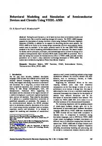
II. Behavioral Modeling The goal of this section is to show "What is modeling of EM devices?". It is given by the definition of abstraction levels in top-down design/bottom-up verification methodologies [2]. In the methodology, the analog and digital parts interact each other at the multi-levels shown in Fig. 1. Since EM devices are defined as the circuits which have the electromagnetic effects, they are classified into analog domain as shown in Fig. 1(b). In the analog domain, at the functional level, the signal flow is described by mathematical functions. At the behavioral level, these mathematical functions are replaced by a number of high-level blocks, i.e., linear transfer function, op-amp, A/D converter, and so on. At the macro level, macromodels are constructed by elementary components such as resistor, capacitor, and nonlinear/linear control source, and second-order effects (slew rate, finite gain, and so on). Finally, at the circuit level, the circuit is decomposed into its elementary components. EM devices are governed by the Maxwell’s equations. On an assumption, they are formulated by lumped components, then, dealing with the EM devices is the same with the analog case shown in Fig. 1(b). However, the present issue what we see says that such a formulation is not sufficient due to the physical effect of the EM device. Alternatively, the macro and behavioral models should be constructed from a differential algebraic equations obtained by discretizing the
behavioral level functional level register-transfer level behavioral level functional level macro level gate level circuit level transistor level
(a)
(b)
Fig. 1. Abstraction levels. (a) Digital case. (b) Analog case.
top-down design/bottom-up verification methodologies [1]. Since the proposed model covers the physical effect of EM devices, it relaxes the gaps between design abstractions and detail so that it is a merit. Further, if a user wishes, the low order model is also available according the approximation fidelity.
III. Selective Orthogonal Matrix Least-Squares Method The selective orthogonal matrix least-squares method is provided in this section. Using a numerical method for analyzing an EM device, the parameter matrix to the multi-port network shown in Fig. 2 is yielded by sampled data in the frequency-domain. After the sampled data were obtained in the time-domain, it is transformed to the ones in the frequency domain by using FFT. The least-squares method converts the parameter matrix into a rational matrix of complex s, where degree of the rational matrix can be determined taking account into the approximation fidelity. A.
I1 V1
EM Device Ii Vi
In
Before constructing the rational matrix, each element of the parameter matrix is separately approximated by a rational function. The poles obtained from all rational functions are used for forming the basis of the rational matrix in the second level data fitting. At a frequency point sq, each element is enforced as
Vn
Yij ( sq ) =
b0 + b1sq + b2 sq2 + L + bm sqm 1 + a1sq + a2 sq2 + L + an sqn
.
(1)
(q = 1, L, H )
Fig. 2. Multi-port network for EM device. Maxwell’s equations. When the reduced-order modeling method as [7] is adapted to these equations, the macromodels of EM devices are obtained. As the EM solvers, some methods such as method of moments (MoM), finite element (FEM) method, and finite difference time domain (FDTD) method are known. These methods are properly used according to the purpose. However, the reduced-order modeling is not applicable to every method. On the other hand, using these EM algorithms, multi-port networks for the EM devices as shown in Fig. 2 are characterized by sampled data using one of the admittance, impedance, and scattering matrices. Then, if the sample data is expressed by a continuous function, it can be used as the macromodel. This paper presents a method for converting the sample data into a rational matrix of s. Depending on the order of the rational function, the approximation fidelity ranges from the physical effect to the minimum expression, and the macromodel is obtained by a linear transfer function. Therefore, the macromodel can be also used for the behavioral model, although circuit information as voltage and current is not considered in general at behavioral level. Nowadays, gaps between design abstractions and detail in physical effect are posing a problem with progress of the
First Level Data Fitting
The approximation is carried out using the weighted least-squares method. However, when the approximation covers a wide range, the method sometimes becomes ill conditioned. Therefore, the frequency range must be partitioned into some regions, and the sampled data is approximated in each region. B.
Second Level Data Fitting
From nature of a parameter matrix, close poles within a distance are found in the first level data fitting. Also unstable poles can be sometimes found. Their poles must be eliminated. All poles except for the duplicated and unstable ones are used to approximate the sample data. Then, the following relation is enforced N
Y ( sq ) = K 0 + ∑ l =1
1 Kl s q − pl
(2)
(q = 1,L, H )
where K, pl, and Y(sq) are the residue matrix, pole, and parameter matrix obtained from the electromagnetic analysis,
C.
2–norm
respectively. The rational matrix in (2) is generally redundant, and one probably desires a more compact model. To achieve it, we need to take account into the approximation fidelity. The next subsection gives the metric of the least squares-method to enforce (2).
10
Normal
0
Metric of Orthogonal Matrix Least-Squares Method
To enforce (2), the following overdetermined matrix equation is solved. PK = Y
Selective –5
10
(3)
0
where K = [ K 0 , K 1K, K N ]T Y = [Y ( s1 ), Y ( s2 ), K, Y ( s q )]
T
(4)
and P is the coefficient matrix adequately constructed from (2). (3) is solved using the QR decomposition: P = WA
(5)
where W and A are orthogonal and upper triangle matrices. Then, the solution K can be written by G = (W TW ) −1W T Y .
(6)
100
degree
200
Fig. 3. 2-norm of residue matrix in matrix least squares-method, where “Selective” is the proposed method and “Normal” is non-selective case. Theorem1:
the
sequence
Z1 2 , Z 2 2 , K, Z M
is
2
monotonously decreasing. Prof) From (9), the following equation is satisfied. (11)
Z sT Z s = Z sT−1 Z s −1 − w sT w s g s g sT
For x ≠ 0 , the quadratic form of (11) is written by
−1
K=A G
The process (6) is called the orthogonal least-squares method [6]. The rest part of this subsection gives the metric of the method in order to take account into the approximation fidelity. The matrices P and W are rewritten using the column vectors as P = ( p1 , p2 , K, pn )
(7)
W = (w1 , w 2 , K, w n ) .
(8)
x T Z sT Z s x = x T Z sT−1 Z s−1 x − wsT ws x T g s g sT x .
Dividing (12) with x T x , the maximum value is written by max x ≠0
max
For M ≤ n , we define the residual matrix to (3) as
Then, the product Z Z M relation T M
(9) is satisfied with the following
~ x T Z sT Z s x ~ x T Z sT−1 Z s −1 ~ x x T g gT ~ x = − w sT w s ~ Ts ~s . T~ T ~ x x x x x x (13)
Putting
x ≠0
Z M = Y − WM GM .
(12)
x T Z sT Z s x xˆ T Z sT−1 Z s−1 xˆ = xT x xˆ T xˆ
(14)
the following inequality is satisfied. xˆ T Z sT−1 Z s−1 xˆ ~ x T Z sT−1 Z s−1 ~ x ≥ T ~ xˆ xˆ xT ~ x
(15)
As a result, the inequality
M
Z MT Z M = Y T Y − ∑ wiT wi gi giT . i =1
(10)
( M = 1, 2, K , n)
The 2-norm of the residual matrix holds the following theorem.
max x ≠0
x T Z sT−1 Z s−1 x x T Z sT Z s x > max x ≠0 xT x xT x
is given, which means
Z s −1
2
> Zs
2
(16)
. Therefore, Theorem 1
is complete. □
[d
into the 2-norm of residual matrix and is orthogonalized at each step, which is corresponding to “Selective’’, the 2-norm is reduced more quickly than the non-selective case (Normal). Therefore, we can avoid the redundancy of (2) by setting a criterion for the 2-norm, which is a fundamental idea of the selective orthogonal matrix least-squares method. The method generalizes the Chen’s method [6] that is a method for identifying a single input single output system. The selective orthogonal matrix least-squares method is applied only to the problem with real coefficient matrix, whereas the constraints (2) are complex. Thus, the matrix equation (5) must be rewritten so that it may have real coefficient matrix. Here, the matrix K of (3) is rewritten by
S1 S2 R1 I1 R2 I2] Shift+ Orthogonalization
[d
S2 S1 R1 I1 R2 I2] Shift+Orthogonalization
[d
S2 R1 S1 I1 R2 I2] Shift
[d
S2 R1 I1 S1 R2 I2] End, if
[d
Zs
2