Behavioural Models of Technological Change

Behavioural Models of Technological Change Paolo Zeppini

ISBN 978 90 3610 260 5 Cover design: Crasborn Graphic Designers bno, Valkenburg a.d. Geul

This book is no. 513 of the Tinbergen Institute Research Series, established through cooperation between Thela Thesis and the Tinbergen Institute. A list of books which already appeared in the series can be found in the back.

Behavioural Models of Technological Change

ACADEMISCH PROEFSCHRIFT

ter verkrijging van de graad van doctor aan de Universiteit van Amsterdam op gezag van de Rector Magnificus prof. dr. D.C. van den Boom ten overstaan van een door het college voor promoties ingestelde commissie, in het openbaar te verdedigen in de Agnietenkapel op dinsdag 13 december 2011, te 12.00 uur

door

Paolo Zeppini

geboren te Pisa, Itali¨e

Promotiecommissie:

Promotors:

Prof. dr. C.H. Hommes Prof. dr. J.C.J.M. van den Bergh

Overige leden:

Dr. C.G.H. Diks Prof. dr. K. Frenken Prof. dr. L. Marengo Prof. dr. A. Soetevent Dr. J. Tuinstra

Faculteit der Economie en Bedrijfskunde

A Mattia e Maia

Acknowledgements It is one of my best virtues, I believe, to work with people who are very good at their job. This was the case with the CeNDEF group and the Tinbergen Institute, which in different times and ways were the house of my doctoral experience. Beside this, I had the opportunity to write my own research project, which often put me in the need of help and advice on various issues. As a consequence, I feel indebted to a large number of people. The most important figures are my two supervisors, prof. Cars Hommes and prof. Jeroen van den Bergh. Their joint supervision was very balanced and complementary. Jeroen introduced me to economics research, starting already in the time of my Tinbergen MPhil. Cars hosted me in CeNDEF, trusting me and my quite exotic research project. Although one can trace Cars’ and Jeroen’s hand in the different chapters of my thesis, I often benefited from their double feedback. I am thankful to the members of my thesis committee, and not just because they accepted to read the manuscript: I had several useful discussions with them over the last three years. First of all prof. Koen Frenken, whom I met at a summer school in late 2008. Starting from comments and advise on my early work, Koen has followed quite closely the development of my thesis. I am particularly thankful to Koen because comments and advise became an invitation to become his co-author and then in the opportunity to engage in post-doctoral work on the complexity and dynamics of technological change. I am indebted to Prof. Luigi Marengo, for comments and suggestions on early versions of my work in this thesis. Jan Tuinstra gave me guidance and supervision during the initial vii

stage of chapter 3: the idea of this chapter was conceived during his course in Bounded Rationality. Similarly I am thankful to Adriaan Soetevent: chapter 5 started as a research proposal written for his course in Social Interactions. I am thankful to Cees Diks, finally, who provided an extensive and detailed feedback on the thesis. The Tinbergen MPhil program thought me the fundamentals of economics. CeNDEF has pursued this educational path, with its focus on non-linear economics, and resulted an ideal habitat for someone like me coming from physics and finance. In one way or another, all members of this group have taught me something, or helped on various issues: Daan, Domenico, Florian, Pim, Marco, Marius, Maurice, Misha, Roald, Saeed, Tatiana, Te. A special thank to Daan, for translating the summary of my thesis in Dutch, to Tatiana, for her guidance in the final stage of the thesis, and to Te, my office mate in the last two years. Visitors to which I am grateful for friendship and help are Jacob, Mei and Yao. Beside teaching me things, CeNDEF people always provided with interesting opportunities for discussion, usually in the coffee room. Topics could range from football champions league to the Harsanyi purification theorem. Roald, Marius and Pim were particularly active in this sense. I am happy to have been the teaching assistant of Roald and Maurice for their game theory courses: I believe I learned a lot from them. I also thank Andries, Ida and Kees from the secretarial office of the Quantitative Economics department. There are other people outside CeNDEF that have been important during my PhD. In particular Volker, who has helped me on several occasions with Matlab and LaTeX, beside being my flatmate and friend. Other important friends in Amsterdam are Zoltan, Karolina, Julian. I want also to mention former colleagues in the Tinbergen MPhil program, who shared with me the intense experience of courses and exams: Jona, Lukasz, Marcelo, Marloes, Matija, Melinda, Michal, Pawel, Petr, Robert, Thomas. Finally, I want to thank my parents, who have taught me to love knowledge and hard work, and Simona, who is actually the responsible for the big turn in my life that transformed me from a financial trader into (maybe) an economist.

viii

Per aspera ad astra

Contents

1 Introduction

1

1.1

Technological change . . . . . . . . . . . . . . . . . . . . . . . . . . . . . .

1

1.2

Thesis outline . . . . . . . . . . . . . . . . . . . . . . . . . . . . . . . . . .

3

1.3

A behavioural approach to technological change . . . . . . . . . . . . . . .

5

1.4

Positive and negative feedback . . . . . . . . . . . . . . . . . . . . . . . . .

7

2 Optimal diversity in investments with recombinant innovation

11

2.1

Introduction . . . . . . . . . . . . . . . . . . . . . . . . . . . . . . . . . . . 11

2.2

The model . . . . . . . . . . . . . . . . . . . . . . . . . . . . . . . . . . . . 15

2.3

2.4

2.2.1

General framework . . . . . . . . . . . . . . . . . . . . . . . . . . . 15

2.2.2

The effect of balance . . . . . . . . . . . . . . . . . . . . . . . . . . 18

2.2.3

Introducing a size effect . . . . . . . . . . . . . . . . . . . . . . . . 22

Optimization of diversity . . . . . . . . . . . . . . . . . . . . . . . . . . . . 26 2.3.1

A simple case . . . . . . . . . . . . . . . . . . . . . . . . . . . . . . 26

2.3.2

Optimization with a size effect and zero initial values . . . . . . . . 32

2.3.3

The effect of non-zero initial values on the optimal investment decision 36

2.3.4

Heterogeneous returns to scale . . . . . . . . . . . . . . . . . . . . . 39

Conclusion . . . . . . . . . . . . . . . . . . . . . . . . . . . . . . . . . . . . 40

2.A Condition for constant balance . . . . . . . . . . . . . . . . . . . . . . . . . 43 2.B General model solution . . . . . . . . . . . . . . . . . . . . . . . . . . . . . 44 xi

3 Competing recombinant technologies for environmental innovation

49

3.1

Introduction . . . . . . . . . . . . . . . . . . . . . . . . . . . . . . . . . . . 49

3.2

The model . . . . . . . . . . . . . . . . . . . . . . . . . . . . . . . . . . . . 52

3.3

3.4

3.2.1

Competing clean and dirty technologies . . . . . . . . . . . . . . . . 52

3.2.2

Recombinant innovation . . . . . . . . . . . . . . . . . . . . . . . . 54

3.2.3

Network externalities . . . . . . . . . . . . . . . . . . . . . . . . . . 56

3.2.4

Arthur’s model extended . . . . . . . . . . . . . . . . . . . . . . . . 56

3.2.5

Simulation of the model . . . . . . . . . . . . . . . . . . . . . . . . 59

Environmental policy . . . . . . . . . . . . . . . . . . . . . . . . . . . . . . 62 3.3.1

Simulation of the model with environmental policy . . . . . . . . . 63

3.3.2

Cost of environmental policy . . . . . . . . . . . . . . . . . . . . . . 68

Conclusion . . . . . . . . . . . . . . . . . . . . . . . . . . . . . . . . . . . . 70

4 A behavioural model of endogenous technological change

73

4.1

Introduction . . . . . . . . . . . . . . . . . . . . . . . . . . . . . . . . . . . 73

4.2

Costly innovators versus cheap imitators . . . . . . . . . . . . . . . . . . . 77 4.2.1

The model . . . . . . . . . . . . . . . . . . . . . . . . . . . . . . . . 77

4.2.2

Steady states and stability . . . . . . . . . . . . . . . . . . . . . . . 81

4.2.3

Period doubling and period halving bifurcations . . . . . . . . . . . 83

4.3

Asynchronous updating of strategies

4.4

Technological progress . . . . . . . . . . . . . . . . . . . . . . . . . . . . . 92

4.5

. . . . . . . . . . . . . . . . . . . . . 88

4.4.1

The model . . . . . . . . . . . . . . . . . . . . . . . . . . . . . . . . 93

4.4.2

Numerical simulations . . . . . . . . . . . . . . . . . . . . . . . . . 98

4.4.3

Path-dependence and learning curves . . . . . . . . . . . . . . . . . 101

Conclusion . . . . . . . . . . . . . . . . . . . . . . . . . . . . . . . . . . . . 105

4.A Proofs . . . . . . . . . . . . . . . . . . . . . . . . . . . . . . . . . . . . . . 107 4.B Conditions for chaotic dynamics . . . . . . . . . . . . . . . . . . . . . . . . 107 xii

5 Competing technologies: a discrete choice model

109

5.1

Introduction . . . . . . . . . . . . . . . . . . . . . . . . . . . . . . . . . . . 109

5.2

Social interactions and network externalities . . . . . . . . . . . . . . . . . 114

5.3

Competing technologies with an environmental policy . . . . . . . . . . . . 121

5.4

Competing technologies and technological progress . . . . . . . . . . . . . . 126

5.5

Technological progress and environmental policy . . . . . . . . . . . . . . . 133

5.6

Conclusion . . . . . . . . . . . . . . . . . . . . . . . . . . . . . . . . . . . . 140

5.A Analysis of equilibria in the basic model . . . . . . . . . . . . . . . . . . . 143 5.B Environmental policy with pollution tax . . . . . . . . . . . . . . . . . . . 144 5.C Analysis of equilibria for the extended models . . . . . . . . . . . . . . . . 144 6 Conclusions

147

6.1

Summary . . . . . . . . . . . . . . . . . . . . . . . . . . . . . . . . . . . . 147

6.2

Future research . . . . . . . . . . . . . . . . . . . . . . . . . . . . . . . . . 151

Bibliography

153

Samenvatting

163

xiii

Chapter 1 Introduction 1.1

Technological change

Technological change is an important driver of economic change which in turn affects human welfare. In addition, it can contribute to solving pressing environmental problems. This requires policies which are based in a good understanding of the mechanisms underlying technological change. Early models of economic growth assumed that technological change occurs in a linear uni-directional way, from science to society, as in Solow (1956). Later studies recognized that technological innovation is often shaped by its users, be they consumers or suppliers of technological products (Dosi et al., 1988). The recognition of the endogenous character of technological change gave place to two alternative streams of studies in economics: endogenous growth theory in neoclassical economics (Romer, 1990; Aghion and Howitt, 1992) and a class of models in evolutionary economics (Nelson and Winter, 1982; Dosi, 1988). The neoclassical approach of endogenous growth theory relies on the concept of the production function, while evolutionary economics describes a population of firms (and consumers) and stresses the heterogeneity of these. This thesis proposes a behavioural approach to technological change, focusing on technological competition and the non-linear dynamics that stems from the endogenous

interplay of heterogeneous actors and technological diversity. In this sense it links up with the evolutionary economics approach.

In both neoclassical and evolutionary economics as well as in the field of innovation studies, there are two rather distinct typologies of models of technological change. First, one class of models deals with the diffusion of innovation (Mansfield, 1961; Bass, 1969; Geroski, 2000) or with technology competition (David, 1985; Katz and Shapiro, 1985; Arthur, 1989). Here a fixed set of technologies is assumed, which do not change during the time horizon considered. A second class of models addresses technological innovation (including invention), either as expanding variety and horizontal differentiation (Romer, 1990; Aghion et al., 2001) or as an improvement of the profitability of an existing technology (Iwai, 1984; Romer, 1986). Relatively few models consider both processes, that is technology diffusion together with technological progress, although in the economy these two processes are strongly interactive. One example is Soete and Turner (1995).

The main focus of this thesis is the study of technology innovation and diffusion in the context of technology competition, when more than one technology or technological choice is available to decision makers (firms). This is done within a behavioural approach, with models that describe the agents’ decision processes and the emergent pattern of technologies. The double perspective of technology diffusion and technological progress is important especially in the context of “environmental innovation policy”. The role of technological innovation in environmental economics and policy has been addressed only recently. From an evolutionary perspective, examples are van den Bergh (2007) and Faber and Frenken (2009), while in neoclassical economics we find a computational general equilibrium approach, as in Bosetti et al. (2009) and the recent theoretical contribution of Acemoglu et al. (2009). Two out of four chapters in the present dissertation model explicitly an environmental policy, and propose a behavioural approach to the interplay of technological change and environmental policy. 2

1.2

Thesis outline

Chapter 2 of this thesis addresses technological diversification in the presence of recombinant technological innovation. Assuming that two (or more) technologies can “recombine”, giving birth to a third innovative technology, a firm’s investment decision is affected by the trade-off between the advantages of specialization (increasing returns) and the benefits from recombinant innovation. The chapter proposes a theoretical cost-benefit analysis of this investment decision problem, deriving conditions for optimal diversity under different regimes of returns to scale. Threshold values of returns to scale and the recombination probability define regions where either specialization or diversity is the best choice. When the investment time horizon is beyond a threshold value, a diversified investment strategy is the best choice. This threshold will be larger for higher returns to scale. Chapter 3 extends the previous model to a dynamic framework, addressing the competition of possibly recombining technologies. The R&D investment decision takes place in a sequential manner, allowing to study stylised facts such as path dependence of technological trajectories and lock-in into one of multiple equilibria. The sequential decisions are described by an urn model based on Polya processes (a type of Markov process) as in Arthur et al. (1987). The innovative contribution of this chapter is to extend Arthur’s model of competing technologies with the concept of “recombinant innovation” (van den Bergh, 2008). The probability of recombinant innovation enters the mechanism of endogenous competition and counterbalances the positive externality of increasing returns to investment. A second extension is the introduction of pollution intensities for the competing technologies, and an environmental policy that charges a price for polluting. The costs of the environmental policy are also considered, with a growth-depressing factor. Numerical implementations of the model allow to study a number of different scenarios with a Monte Carlo approach, by looking at the distribution of final outcomes. In particular, one can thus evaluate the combination of environmental regulation and recombinant 3

innovation. In Chapter 4, firms’ behavioural heterogeneity is addressed with an analytically tractable model of the competition between a superior but costly technology and an inferior free technology. This model is inspired by the Schumpeterian dynamics model of Iwai (1984) and by the model of costly optimizers versus cheap imitators of Conlisk (1980). The theoretical strategy-switching framework is the discrete choice model of Brock and Hommes (1997). Adopters of the superior technology (innovators) pay a price to reduce their production cost, while the others (imitators) maintain the production cost level of the inferior technology. The basic idea is that imitation works better the more innovators are around, with a trade-off between the advantages of the two strategies. Asynchronous updating reproduces the more realistic scenario where agents only gradually change their strategy. The model is upgraded with a mechanism of knowledge cumulation, which describes the advancement of the technological frontier resulting endogenously from agents’ innovation decisions in each time period. Put differently, Chapter 4 proposes a behavioural approach to model endogenous technological progress. Chapter 5 consists of a discrete choice model of technology competition in line with Brock and Durlauf (2001). The model builds on the interaction of three factors: technological and social externalities, technological progress and environmental policy. A basic version of the model serves to study the equilibrium structure of technology competition. Technological progress and environmental policy are introduced separately and then brought together in the final version of the model. Environmental policy concerns cases where a “clean” and a “dirty” technology compete for adoption and investment. In this case the main interest is in the conditions that enable the market to escape a locked-in dirty technology by tipping the system from the “bad” to the “good” equilibrium where the clean technology is dominant. In this sense, the model provides insights into how decision externalities, technological progress and policy stringency interact and affect the path towards this target. 4

Technology competition is tackled from different angles in different chapters. Chapter 2 and Chapter 3 focus on the concept of recombinant innovation, the first being a costbenefit analysis in a static environment, while the second extending the decision framework to many time periods, with a sequential decision framework. Chapters 4 and 5 study the dynamics of technology decisions in a discrete choice setting, and look at technological progress as cost reduction or profitability improvement. Put differently, chapters 2 and 3 address horizontal innovation, with the advent of a third technology, while chapters 4 and 5 deal with vertical innovation, which is about performance improvements of given technologies. Finally, chapters 3 and 5 introduce an environmental economic analysis, taking into consideration the role of an environmental policy that affects technology choices. Table 1.1 summarizes the type of technological progress considered in each chapter, and whether environmental economics issues are addressed.

Chapter Chapter Chapter Chapter

2 3 4 5

Horizontal technical progress yes yes no no

Vertical technical progress no no yes yes

Environmental policy no yes no yes

Table 1.1: Main themes of the thesis chapters.

1.3

A behavioural approach to technological change

This thesis is about the decision making process that underlies technology competition and its dynamics, and the main actor in such decision process is the firm. The focus on agency and dynamics is an important departure from neoclassical models of endogenous technical change, as Romer (1990) and Aghion and Howitt (1992). Aggregation of individual decisions turns into technology competition and, possibly, technological progress, at the macro-level. This way to describe technological change as an emergent property of dynamically interacting agents is inspired by behavioural models of financial markets seen 5

as complex evolutionary systems. For a survey of such models see Hommes and Wagener (2009) and Hens and Schenk-Hopp´e (2009). The focus on decision making and agency leads to dynamic models, apart from the case of Chapter 2. In this chapter time only plays the role of a parameter indicating the time horizon of the investment. All other chapters present a dynamic setting, where agents make decisions in each time step, be this in a sequential manner as in Chapter 3 or at the same time in each period, as in the discrete choice models of chapters 4 and 5. The application of a discrete choice framework and a logit dynamics to technology competition is one of the contributions of these two chapters. A second contribution of these two chapters is to introduce technological progress in the process of technology competition. Technological progress arises endogenously through a knowledge cumulation process. The latter depends on the time pattern of agents’ technology choices. This allows one to model endogenously vertical technological progress, because agents choose between lower or higher production costs (Chapter 4), and lower or higher profitability (Chapter 5). Horizontal differentiation of intermediate goods is not invoked to trigger the endogenous mechanism of technical progress, as it is the case in Romer (1990) and Aghion and Howitt (1992). This is a second difference with respect to these models. A recent stream of literature studies the effects of social interactions on the process of innovation adoption and consequently on the diffusion pattern of innovation. Examples are Manski (2006), Young (2009) and Brock and Durlauf (2010). In Manski (2006) there is a focus on dynamics, which is studied with a computational approach. The main research question is the role of cohorts in innovation diffusion. Young (2009) studies the effect of different typologies of social effects on the adoption time curve, namely contagion, social influence and social learning. Adoption curves are studied also in Brock and Durlauf (2010), with a focus on expectations consistency and equilibrium, instead of dynamics. In all these models there is one technological innovation under study, and the main issue is the timing of its adoption. The present dissertation addresses technological change in 6

a more complex setting, first by enlarging the set of technologies available for adoption, with technology competition, and second by introducing technological progress. Another challenge of the discrete choice models in chapters 4 and 5 is to reproduce the variability of technology markets with simple deterministic models, through the occurrence of chaotic dynamics. Irregular technology fluctuations then have an endogenous explanation. In chapters 2 and 3 instead, the notion of uncertainty of the innovation event is present, with the probability of recombinant innovation. In Chapter 2, this probability is endogenously dictated by agents’ choices, so that it turns out to be a deterministic factor. In Chapter 3, agents choices follow a stochastic process, which renders the probability of innovation a stochastic factor. The dynamic models of chapters 3, 4 and 5 all adopt a bounded rationality approach. A survey of bounded rationality is found in Conlisk (1996). The idea of bounded rationality is present in two ways. First, agents may make decisions only based on past experience. Second, agents’ vision or ability to choose the option that performed better in the past is limited. In the discrete choice models of chapters 4 and 5 the last concept is expressed by the intensity of choice parameter (Hommes, 2006), measuring how easily agents switch to the best performing strategy. This parameter has a counterpart in a parameter of the urn model of Chapter 3, so that a link is found between the discrete choice models `a la Brock and Hommes (1997) and the urn models of Arthur et al. (1987).

1.4

Positive and negative feedback

A number of stylised facts of technology dynamics, such as path dependence, lock-in, multiple equilibria, critical transitions, learning curves, can be explained with the endogenous mechanisms of the agents’ decision process. More specifically, such stylised facts arise as emergent properties of decision feedback loops. Decision feedbacks can be negative or positive, depending on whether the marginal effect of one agent choosing one option gives a positive or a negative contribution to the utility of agents choosing the same option, 7

respectively. For this reason, the feedback takes the form of an externality in one agent’s decision. The literature on technological change and technology competition has addressed different sources of positive feedback, as for instance economies of scale (Mansfield, 1988), network externalities (Arthur, 1989) and learning-by-doing (Arrow, 1962). A comprehensive study of positive externalities in the economy is done by Arthur (1994). Whenever technology decisions are affected by motives and incentives other than technological performance, there can be also negative feedbacks. One example is when technologies have an impact on the environment. Polluting technologies are characterized by a negative externality (Stern, 2007). An environmental policy internalizes the negative externality of pollution with a tax on pollution or with a subsidy for clean technologies, giving place to a negative feedback in agents’ decision about polluting technologies. A different perspective on positive and negative feedbacks in the economy is offered by the concept of super-modularity (positive feedback) and sub-modularity (negative feedback). These concepts have been proposed in models that describe firms’ output decisions in a strategic environment (see for instance Milgrom and Roberts (1990)). This thesis does not deal with strategic behaviour, because of two major assumptions: first, agents only consider past experience in making a decision; second, the economic systems addressed always present a large number of agents, and the marginal effect of an individual decision is negligible. Decision feedbacks inhabit all dynamic models in this thesis, namely the models of chapters 3, 4 and 5. Positive feedback is modelled explicitly in chapters 3 and 5, with its effect being proportional to the share of one technology in the market. The rationale for this feedback is that a technology becomes more attractive as more firms implement it, cutting down costs (economies of scale), as more agents use it, because of technology standards and infrastructures (network externalities), and as it becomes more efficient due to its application (learning by doing). A further source of positive externality that is invoked 8

in Chapter 4 are social interactions (Manski, 2006; Young, 2009; Brock and Durlauf, 2010). These can give place to positive feedback whenever the technology adoption decision is driven also by “word of mouth” via a contagion effect or by a recruitment process (Kirman, 1993), or as conformity effects and habit formation (Alessie and Kapteyn, 1991). Social interactions by no means lead always to positive feedback: conspicuous consumption gives place to a snob effect (Frank, 2005), where an increasing number of adopters becomes a reason not to adopt, instead of to adopt. For technology choices this is not likely to be the case, and the models of chapters 3 and 5 assume that also social interactions lead to positive feedback. Chapters 3 and 5 consider also a source of negative feedback with the introduction of an environmental policy that internalizes the negative externality from pollution of technologies. This is done with a tax on pollution (Chapter 3) or with a subsidy for the clean technology (Chapter 5). The introduction of the negative feedback of an environmental policy beside the positive feedback of technology decisions explained above give place to a complex system of decision feedbacks in the models of chapters 3 and 5. The model of Chapter 3 presents a further decision feedback from the probability of recombinant innovation. This feedback may be either positive or negative depending on the diversity of the technology market, that is on the distribution of the market shares of competing technology. The probability of recombinant innovation is assumed to depend positively on the diversity of the market, being maximum for equal technology shares. Whenever one technology becomes dominant, the probability of recombinant innovation decreases. This represents an incentive to re-balance the market, choosing the technology with lower market share. Technology decisions may also be characterized by a negative feedback from the price reduction effect of technological innovation. This is the fundamental idea of the model of Chapter 4. Here the endogenous market dynamics of supply and demand is modelled, so that also the market price affects agents’ decision. In particular, as more agents 9

choose the superior technology (more innovators), the price falls due to cost reduction, and so do profits from sales, which depend positively on the price. Lower profits hurt more innovators than imitators, because of the fixed cost of innovation. This mechanism translates into a negative feedback, where the utility from innovation decreases as more agents innovate. Table 1.2 summarizes the arguments above, reporting the type of decision feedback in the dynamic models proposed in the thesis (Chapter 2 is not considered because it contains a static model). feedback Chapter 3 positive and negative Chapter 4 negative Chapter 5 positive and negative Table 1.2: Different types of decision feedbacks in the chapters with a dynamic model.

10

Chapter 2 Optimal diversity in investments with recombinant innovation 2.1

Introduction

When organizations decide on investment in technological innovation, they implicitly or explicitly make choices about diversity of options, strategies or technologies. Such choices should ideally consider the benefits and costs associated with diversity and arrive at an optimal trade-off. One important benefit of diversity relates to the nature of innovation, which often results from combining existing technologies or knowledge bases (Ethiraj and Levinthal, 2004). For instance, the laptop computer combines microelectronics, display technology and a battery; the windmill is a combination of water mill technology and the idea of a sail; the laser is quantum mechanics integrated into an optical device; and the optical fibre used in telecommunication is a laser applied to glass technology. Innovative combinations apply especially to technologies that are relatively close to each other in technology space, such as is common in the bio-pharmaceutical industry and the software industry. Indeed, many multi-product firms choose products in such a way that they can enjoy the spillover effects of learning and innovation. This chapter is a version of Zeppini and van den Bergh (2008).

Here we propose a theoretical framework for the description of a generic innovative process resulting from the interaction of two existing technologies. The interaction will depend on how these two options match. The ultimate aim of the model is to assess the optimal diversity of technological investments in the context of modular innovation. The main idea is that, in an investment decision where available options may recombine and give birth to an innovative option (technology), some degree of diversity of parent options can lead to higher benefits than specialization. This problem is relevant to both private and public organizations. In addition, the recombinant view of technological innovation can help to explain the diversification pattern of firms and their size distribution, thus contributing to the debate initiated by Penrose (1959). A motivation for our model is the recent attention for a socio-technological transition to large scale use of renewable energy (Geels, 2002; van den Bergh and Bruinsma, 2008). Diversity here is related to lock-in of an inferior or undesirable technology, such as fossil-fuel-based electricity generation that contributes considerably to global warming. A diversity analysis of energy systems provides insights into the appropriate level of diversity that should be aimed for or maintained in different phases of an energy transition (van den Heuvel and van den Bergh, 2008). One might distinguish between a bipolar model of recombinant innovation where the two elements being combined are somehow balanced in terms of complexity or importance (e.g., electric and combustion engines in a hybrid car) and a case where an existing complex technology is improved by adding a small, less important or less complex element (e.g. installing a navigation system into a car). The latter is perhaps often seen as an ordinary, gradual innovation, whereas the first case, which we address in the present article, is more associated with major or even radical innovations. Even the restricted set of bipolar recombinant innovations is quite large: the jet engine resulted from combining internal combustion and the turbine concept. In the power generation sector, there are systems that combine different ways of energy transformation, such as photovoltaic 12

collectors using the heat radiation produced by combustion in a gas turbine. Other examples of recombinant innovation are electronic devices like smartphones and ebooks, which integrate pre-existing technologies in a modular way. Usually in economics and finance, diversity is seen as conflicting with efficiency of specialization. Such efficiency is claimed on the basis of increasing returns to scale arising from fixed costs, learning, network and information externalities, technological complementarities and other self-reinforcement effects. Arthur (1989) studies the dynamics of competing technologies in cases where increasing returns cause path dependence and selfreinforcement, possibly leading to lock-in. This can be seen as a descriptive or positive approach to understanding the dynamics of systems in the presence of positive feedback. Our approach instead is normative, in that it studies the efficiency of the system of different options, considering total net benefits of technologies over time, including innovation-related and scale-related effects of diversity. A theoretical framework for the study of optimal diversity was proposed by Weitzman (1992) in the context of investment projects for biodiversity protection. The positive role of diversity is recognized in option value and real option theories, which clarify when to keep different options open in the face of irreversible change and uncertain circumstances (Arrow and Fisher, 1974; Dixit and Pindyck, 1994). However, these theories treat diversity as exogenous and do not consider innovation, whereas our model treats diversity as endogenous and contributing to the value of the overall system beyond merely keeping decisions open. Similarly, portfolio theory (Markowitz, 1952; Sharpe, 1964), another classical approach to investment decisions, excludes the possibility of innovation. Moreover, returns to scale are not part of this theory, so that diversification is the usual optimal choice. In the case of technological investments, however, the opposition between returns to scale and recombinant innovation may result in a wider range of optimal solutions depending on the relative strength of each effect, as we will show. The relevance of our analysis relates to the myopia of economic agents and organi13

zations. Chiu et al. (2008) study empirically the conditions for a positive link between technological diversification and firms’ performance. In real-world decision making, shortterm interests often prevail, possibly since the advantages of increasing returns are perceived as more clear and certain than the advantages of diversity and recombinant innovation. Fleming (2001) argues that one reason for uncertainty in recombinant innovation is that inventors experiment with unfamiliar technologies and unexploited combinations of technologies. The trade-off between short-term efficiency and long-term benefits from diversity resembles the exploitation versus exploration problem (March, 1991). In fact, recombinant innovation can be regarded as a form of exploration and search. At first sight, diversity benefits as proposed here seem to resemble economics of scope. However, the first notion relates to recombinant innovation, while the second is about synergies in production mainly due to bundled marketing and logistics. Whereas economies of scope are static, diversity benefits are dynamic in nature. A model of diversity connects not only with the research on modularity but also with the approach of evolutionary economics, as expressed by Nelson and Winter (1982), Dosi et al. (1988), Andersen (1994), Frenken et al. (1999) and Potts (2000), among others. The idea of innovation as recombination dates back to Schumpeter (1934). However, evolutionary economics tends to avoid the notions of optimality and efficiency in terms of maximizing a value function. Our approach can, in fact, be seen as combining diversityinnovation ideas from evolutionary economics with optimality and cost-benefit analysis of neoclassical economics. In an evolutionary approach, one talks of a population of parent options and an offspring to refer to the innovative option. Here we will deal with the smallest population possible: namely, only two parent options, so as to keep the model simple and allow for analytical solutions. We propose a theoretical model of recombinant innovation with two parent technologies and address the decision problem of optimal diversification of the associated R&D investment portfolio. The conditions under which diversification or specialization is op14

timal are studied. The main factors of influence on the optimal allocation of investment are the time horizon and the returns to scale. The model builds upon and generalizes the model by van den Bergh (2008) but differs from it in a number of ways. First, whereas the earlier study was based on numerical analysis, here we derive analytical results, both for model dynamics and optimal investment solutions. Second, in contrast to the earlier study, this analysis addresses heterogeneous returns to scale, as well as non-zero and heterogeneous initial values of parent technologies. All this makes it possible to study asymmetry effects in the investment decision. Third, we consider the effect of the (cumulative) size of parent technologies on the probability of recombinant innovation. This chapter is organized as follows. Section 2.2 presents the recombinant innovation model, and provides a solution to the dynamics of the recombinant investment. Section 2.3 addresses the problem of optimal diversity in different cases of growing complexity. Section 2.4 concludes and provides suggestions for further research.

2.2 2.2.1

The model General framework

Consider a system of two investment options that can be combined to give rise to a third. Think of an automotive corporation that is considering the possible benefits of developing a hybrid car. Let I denote investment in the parent options, which in this example are the internal combustion and electrical engines. Investment I3 is devoted to the third (innovative) option, that is, the development of the hybrid car. The latter is the investment in recombinant innovation, which occurs with probability Pe . The growth rates of parent options are proportional to investments, with shares α and 1 − α. Let O1 and O2 represent the values of the cumulative investment in parent options, and O3 the expected value of the innovative option. Recombinant innovation is a binary event: a new option emerges with probability Pe , and nothing happens with probability 1 − Pe . 15

Hence, the expected value is simply Pe times the capital invested in the new option. The dynamics of the system can then be described by the set of differential equations: O˙ 1 = I1 = αI, O˙ 2 = I2 = (1 − α)I,

(2.1)

O˙ 3 = Pe (O1 , O2)I3 .

The optimization problem that we address is finding an α that maximizes the final total benefits from parent and innovative options. In the hybrid car example, this means to maximize the net benefits from the development of the internal combustion engine, the electrical engine, and their integration. We assume for parent options a constant allocation of capital I over time

I1 I2

=

α , 1−α

which results in a constant linear growth (accumulation) of O1 and O2 . The time pattern of the innovative option is non-linear:

O1 (t) = O10 + I1 t, O2 (t) = O20 + I2 t,  t Pe (τ )dτ. O3 (t) = I3

(2.2)

0

We define the probability of emergence of an innovative option Pe as depending positively on the balance B(O1 , O2 ) of parent options.1 Moreover, we assume a positive dependence (with diminishing marginal effect) on the total size of parent options:

Pe (O1 , O2 ) = eB(O1 , O2 )S(O1, O2 ).

(2.3)

The size effect is captured by the factor S(O1 , O2 ), and will be addressed in some length 1

An alternative interpretation of Pe is to think of it not as a probability but simply as a matching factor for a recombinant invention that has already occurred. Consequently, O3 would not be an expected value, while Pe , not being a probability, would not be bounded above and could be larger than 1.

16

in Section 2.2.3. The coefficient e ∈ [0, 1] can be interpreted as the effectiveness of recombinant R&D, which may change due to learning. In general, as clarified by Stirling (2007), e depends on two other dimensions of diversity: namely, variety (the number of parent options) and disparity (how far apart the options are in the technology space). Balance expresses how (un)equal the distribution of different options is in a population: the more balanced a system is, the more diversified it is. The idea is that a more balanced investment has a larger probability of recombinant innovation.2 When one option is zero, we have pure specialization. The balance function must have the following properties: B(O1 , O2 ) ∈ [0, 1], B(O1 = O2 ) = 1 (maximum diversity or perfect balance) and limOi →0 B(Oi , Oj )|Oj =const = 0 with i, j = 1, 2 and i = j. The optimization problem of the investment decision is addressed by considering the joint benefits of parents and innovative options. In order to model the trade-off between diversity and scale advantages of specialization, we introduce a returns to scale parameter si for each technology i = 1, 2, 3. This acts on the cumulative investment in each option, capturing not only economies of scale but also learning over time. For instance, there is a s1 for the investment in internal combustion engine, a s2 for the electrical engine, and a s3 for the hybrid car. The overall benefits from investment can be expressed as: V (α; t) = O1 (α; t)s1 + O2 (α; t)s2 + O3 (α; t)s3 ,

(2.4)

where t is the time horizon of the investment. To find the optimal α, an explicit solution to O3 (α; t) is required, i.e. we need to compute the integral in the third equation of (2.2). 2

This idea is consistent with both codified and tacit knowledge. In the first case, recombination will most likely occur through engineers that are specialised in different technologies exchanging or combining tacit knowledge about these. More balance will then mean more engineers in either technological area and therefore more opportunities to cooperate or exchange information. In the case of codified knowledge, a single individual will be able to combine knowledge about separate technologies. More balance may then go along with better accessibility and quality of codified information in either technological area, which in turn will enhance opportunities for successful recombination by a single researcher. Of course, codified knowledge is flexible in that it also allows recombinant innovation to follow the route of cooperation among individuals with different technological expertise (see van den Bergh (2008)).

17

2.2.2

The effect of balance

A balance function is defined in the positive octant of an n-dimensional space. A functional specification of the balance of two options x and y should have the following properties: 1. it is symmetric in its arguments B(x, y) = B(y, x); 2. the maximum value is attained on the diagonal B(x, x) ≥ B(x, y) ∀x, y ≥ 0; 3. the minimum value (lowest balance) is attained when one of the two options is zero: B(x, 0) = B(0, x) = 0 < B(x, y) ∀y > 0; 4. it is homogeneous of degree zero: B(λx, λy) = B(x, y). The latter means that the balance of two quantities can be expressed as a function of their ratio b = O1 /O2 (simply put λ = 1/x). The functional specification of the balance that we adopt is the “Gini” measure (Fig. 2.1): B(O1 , O2 ) = 1 −

(O1 − O2 )2 O1 O2 =4 . 2 (O1 + O2 ) (O1 + O2 )2

(2.5)

This specification is a rather obvious way of expressing the symmetry of a system, and it is a standard measure of concentration in industrial organization studies.3 Expressed as b a function of the ratio, the above specification reads B(b) = 4 (1+b) 2.

Suppose that the total size of the population of parent options has a negligible effect on the probability of emergence, and set the size factor to the value S(O1, O2 ) = 1 in Eq. (2.3), so that the probability of emergence only depends on the balance B(O1 , O2 ) 3

Notice the differentiability in O1 = O2 . Other specifications are possible, for instance B(O1 , O2 ) = min{O1 ,O2 } 1 −O2 | 1 − |O O1 +O2 and B(O1 , O2 ) = max{O1 ,O2 } (see also Stirling (2007)). A detailed analysis of the latter specification is available upon request. The case O1 = O2 = 0 is excluded by all these specifications. This is a rather degenerate and irrelevant case, however, as we are only interested in systems with at least one option (∃ i = 1, 2 | Oi > 0). Otherwise, we can always define B(0, 0) = limO1 ,O2 →0 B(O1 , O2 ) = 1.

18

1 0.9 0.8 0.7

Balance

0.6 0.5 0.4 0.3 0.2 0.1 0 40 30

Option 2

20 10 0

0

5

20

15

10

25

30

35

40

Option 1

Figure 2.1: Graph of the diversity function with two parent options.

through the proportionality factor e. The value of the innovative option at time t is then:  O3 (t) = 4I3

0



t

Pe (τ )dτ = eI3

0

t



O1 (τ )O2 (τ ) O1 (τ ) + O2 (τ )

2 dτ.

(2.6)

If the initial value of parent options is zero (O10 = O20 = 0), the balance is constant and equal to 4α(1 − α). In this case, the innovative option grows linearly in time. If we allow for positive initial values O10 , O20 , we obtain the following function of time:

B(t) = 4

(O10 + αIt)(O20 + (1 − α)It) , (O0 + It)2

(2.7)

where O0 = O10 + O20 is the total initial size. Notice that limt→∞ B(t) = 4α(1 − α), and B  4α(1 − α) as soon as t  Oi0 /(αI), i = 1, 2. We can then state the following:

Proposition 2.2.1. In the long-run the balance converges to the constant value B(α) = 4α(1 − α), which is independent of the initial values of the parent options. 19

The dynamics of the balance in the transitory phase (t ∼ Oi0 /(αI)) depends on initial conditions and on the investment share α, and can be understood easily by looking at options trajectories in (O1 , O2 ) space. From the first two equations of (2.2) we have: O2 = O20 −

1−α 1−α O10 + O1 . α α

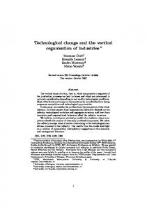
The starting point (t = 0) of each trajectory is determined by the initial values (O10 , O20). The slope is the ratio of investment shares. For our recombinant innovation system we identified seven major cases, which are reported in Fig. 2.2. This figure must be read as follows: the more a trajectory gets close to the line O1 = O2 , the more balanced is the investment, and the larger the probability of recombinant innovation (for a detailed analysis of each of these cases, see Zeppini and van den Bergh (2008)). In principle,

Figure 2.2: Trajectories of the two parent options in (O1 , O2 ) space. Trajectory “1” has O10 < O20 and α < 1/2; trajectory “2” has O10 < O20 and α > 1/2; trajectory “3” has O10 > O20 and α < 1/2; trajectory “4” has O10 > O20 and α > 1/2; trajectory “5” has O10 = O20 and α = 1/2; trajectory “6” has O10 = O20 and α < 1/2; trajectory “7” has O10 = O20 and α = 1/2. For “Constant balance” the slope is equal to the ratio O20 /O10 .

the optimal condition for recombinant innovation is when the balance is constant and maximal (Case 7). In general, for constant balance the following condition applies: 20

Proposition 2.2.2. The balance is constant and equal to B(α) = 4α(1 − α) iff O10 α . = O20 1−α

(2.8)

For a proof of this proposition see Appendix 2.A. This configuration falls into Cases 1, 4 and 7 of Fig. 2.2. As a function of time, the balance may have a critical point t∗ where it reaches its maximum value.4 Fig. 2.3 shows two examples of monotonic and nonmonotonic dynamics. Here we have set I = 4, with initial values O10 = 1 and O20 = 2. 1 Balance 0.95

0.9 2

0.85

0.8

1

0.75

Time 0.7

0

1

2

3

4

5

6

7

8

9

10

Figure 2.3: Two examples for the balance as a time function (I = 4, O10 = 1, O20 = 2). Case 1: α = 1/4. Case 2: α = 3/4.

In Example 2 we have α/(1 − α) = 3: there is a time t∗ = 1/2 when the balance is equal to 1 (a perfectly similar pattern would obtain in Case 3). In Example 1 the balance is decreasing, with α/(1 − α) = 1/4. In general, B(t) is decreasing when and increasing when α 1−α

O20 ) and 2 (α > 1/2 and O10 < O20 ) of Fig. 2.2, when the balance has a critical point t∗ . The convex time pattern occurs when the balance does not have a critical point. For example, take O0 = 3, O10 = 1, O20 = 2, α = 2/3. Since O10 /O20 = 1/2 < α/(1 − α) = 2, we have

t . that option 3 follows a concave time pattern, O3 (t) = 43 2t + ln(1 + t) − 1+t

2.2.3

Introducing a size effect

The size factor S(O1 , O2 ) in expression (2.3) is meant to capture the positive effect that a larger cumulative size has on the probability of emergence, i.e. a kind of economies of scale effect in the innovation process. Such a factor is designed to have the following properties: first, it is increasing in the size of each parent option with marginally diminishing effects. Second, it must be bounded, to guarantee that the probability Pe is 22

in the interval [0, 1]. In addition, it should not overlap with the balance factor, which means that only the total sum of the sizes of options matters and not their distribution. These properties capture increased learning subject ultimately to saturation. We adopt a Weibull cumulative distribution specification: S(O1, O2 ) = 1 − exp[−σ(O1 + O2 )].

Here ∂S/∂Oi = ∂S/∂O = σ/exp(σO), with O =

 i

(2.12)

Oi . The parameter σ captures the

sensitivity of Pe to the size when the balance is kept constant.5 After including the size factor, the probability of emergence (2.3) is expressed as follows:

Pe (O1, O2 ) = 4e

O1 O2 1 − exp[−σ(O1 + O2 )] . 2 (O1 + O2 )

(2.13)

This expression depends on the sum and the difference of O1 and O2 (see Eq. 2.5). As a function of time, the probability of emergence reads

Pe (t) = 4e

(O10 + αIt)(O20 + (1 − α)It) 1 − exp[−σ(O0 + It)] . 2 (O0 + It)

(2.14)

We might think of the event of innovation as occurring suddenly at a time tE , and write Pe (t) = P rob(tE < t). Note how the effect of size on Pe does not depend on whether it comes from “old” value O0 or from “new” investment It. This is not true for the balance.6 The size factor S(t) describes a saturation effect of the probability of emergence Pe . After a sufficiently long time (It  O0 ), the effect of cumulative size on Pe vanishes, since limt→∞ S(t) = 1 and limt→∞ Pe (t) = 4α(1 − α), from Eq. (2.7). In cases other than the symmetric one (α = 1/2), the balance is suboptimal (B < 1), and Pe (t) < 1 ∀t. This is summarized in the following proposition: 5

One could allow for heterogeneous effects with the specification 1 − exp(−σ1 O1 − σ2 O2 ). This can address two different technologies operating in different sectors with different sensitivities σ1 and σ2 . 6 Formally, S(t) is invariant to a time shift t → t∗ , such that O0 + It = O0∗ + It∗ , while B(t) is not.

23

Proposition 2.2.3. When a marginal diminishing size effect is introduced in the probability of emergence, innovation occurs almost surely iff the balance is constant, and the investment is maximally diversified (α = 1/2, B = 1). We now integrate the third equation of the model (2.1) with a full specification of the probability of emergence, taking into account the balance and the size effect together. Before doing this, it is useful to write down the general expression of the probability of emergence as a function of time:

Pe (t) = 4

(O10 + αIt)(O20 + (1 − α)It) 1 − exp[−σ(O0 + It)] . 2 (O0 + It)

(2.15)

We will now proceed in steps in order to better understand the effect of size in the model. First assume the balance is constant, i.e. condition (2.8) holds and B = 4α(1 − α).

The probability Pe then becomes Pe (t) = eB 1 − exp[−σ(O0 + It)] , and we obtain the following time pattern for the innovative option value: 



exp(−σO0 ) exp(−σIt) − 1 . O3 (t) = eI3 B t + σI

(2.16)

The first term of this expression is what we have without the size factor. The second ¨ 3 (t) > 0 ∀t ≥ 0.7 This means the term comes from the size effect. Here O˙ 3 (t) > 0 and O innovative option has a convex time pattern. Such a behaviour accounts for a transitory phase in which the innovation ‘warms up’ before becoming effective. This is a stylised fact of innovation processes (Fig. 2.4).

The time pattern of O3 (t) tends to the asymptote eI3 B t − exp(−σO0 )/σI : after a sufficiently long time, the innovative option attains linear growth. An indication of the characteristic time interval of the transitory phase is given by the intercept tˆ =

exp(−σO0 ) . σI

Interestingly, this characteristic time depends neither on the recombinant innovation ef7

24

¨ 3 (t) = I3 eBσIexp[−σ(O0 + It)]. The first derivative is O˙ 3 (t) = I3 Pe (t), the second derivative is O

120

100

new technology value asymptote

technology value

80

60

40

20

0

0

20

40

60

80

100

120

140

160

180

200

time

Figure 2.4: Value of the innovative option as a function of t, for the case of constant balance. Here α = 1/2, e = 1, I3 = 1, I = 4, σ = 1/400, and O10 = O20 = 2. Then O3 (t) = t + 100e−0.01t(e−0.01t − 1) and the asymptote is t − 100e−0.01 .

fectiveness e nor on the investment I3 . The higher the sensitivity σ or the initial value O0 or the investment rate I, the shorter the transitory phase and the faster the innovative option gets to linear growth. Relaxing the assumption of constant balance, we have to solve the following integral:  O3σ (t)

= 4I3

0

t

(O10 + αIτ )(O20 + (1 − α)Iτ ) 1 − exp[−σ(O0 + Iτ )] dτ. 2 (O0 + Iτ )

We call this solution O3σ (t) to differentiate it from the solution without size effect. Appendix 2.B contains the detailed derivation. The result is:

4I3 exp(−σO0 ) O0 + It σE 2 ln exp(−σIt) − 1 − + O3σ (t) = BI3 t + B σI I O0

 1 4I3 2  1 E 1 − exp[−σ(O0 + It)] + (2.17) 1 − exp(−σO0 ) − − I O0 O0 + It k  k ∞  ∞     − σ(O0 + It) − σO0 4I3  E σ + E(H − F ) − − , I k · k! k · k! k=1 k=1 where B = 4α(1 − α) is the value of the balance when it does not depend on time; 25

E = O10 (1 − α) − αO20 ; F = α; G = −E; and H = (1 − α). When the balance is constant, we have O10 (1 − α) = O20 α, and the expression of O3 (t) only contains the first two terms since E = G = 0. When the balance is not constant, the time pattern of the third option contains a logarithmic term, a negative exponential divided by a linear function, and two infinite sums, one constant and the other dependent on time. As argued in Appendix 2.B, the two sums converge to negative exponentials. This means that the infinite sum which depends on time goes to zero for It  O0 . In the long run, the time pattern of O3σ is given by the following expression: O3σ (t)  4α(1 − α)I3 t − 4

I3 It σ[O10 (1 − α) − O20 α]2 ln . I O0

(2.18)

Without the size effect, we have (see equation (2.11)): O3 (t)  4α(1 − α)I3 t + 4

I3 It [O10 (1 − α) − O20 α](1 − 2α) ln . I O0

When a size factor is present, the logarithmic term adds negatively to the value of the innovative option, producing the expected convex time pattern which reveals the diminishing marginal contribution of parent technologies. Without the size effect, the logarithmic term can be either positive or negative. This shows how a marginally diminishing size effect is important in reproducing the typical threshold effect of recombinant innovations. The contribution of the logarithmic term depends to a great extent on the value of the sensitivity σ, which should be assessed empirically for each context.

2.3 2.3.1

Optimization of diversity A simple case

We now address the problem of optimal diversity maxα∈[0,1] V (α; t), where the objective function is given by (2.4). In general the solution depends on the time horizon. Here 26

we consider different cases, starting from the simplest one, where parent options have zero initial value, there is no size effect, and returns to scale are the same for the three technologies. Later we relax these assumptions. Assume zero initial value for parent options, then O1 (t) = αIt, and O2 (t) = (1 − α)It and the balance is constant. Assume, moreover, no size effect (S = 1). Also the innovative option grows linearly with time: O3 (t) = 4eI3 α(1 − α)t.

(2.19)

Assume, finally, that returns to scale are the same for all three technological options, s1 = s2 = s3 ≡ s. The maximization problem of optimal diversity then becomes:

max V (α; t) = ts I s αs + (1 − α)s + C s αs (1 − α)s ,

(2.20)

α∈[0,1]

where C =

4eI3 . I

This factor weights the contribution of recombinant innovation to total

benefits. This contribution is larger for a larger effectiveness e. It is useful to normalize the benefits function to its value in the case of specialization V (α = 0; t) = V (α = 1; t) = I s ts : V (α; t) V˜ (α) ≡ = αs + (1 − α)s + C s αs (1 − α)s . I s ts

(2.21)

The function V˜ (α) reaches a maximum for α = 1/2 (maximum diversity), or for either α = 0 or α = 1 (specialization). Fig. 2.5 reports the benefits curve (2.21) in the case of increasing returns to scale (s = 1.2) for four different values of the factor e. Either specialization or diversity can be optimal, depending on factor C = 4eI3 /I. If the effectiveness e is insufficiently large, for instance, returns to scale may be too large for diversity to be the optimal choice. This result is in accordance with Dasgupta and Maskin (1987): in an uncertain environment parallelism of investments should not be considered as waste, unless increasing returns outweigh the benefits from diversification. 27

1.1

e=0 e=0.4 e=0.7 e=1

1.05

benefits

1

0.95

0.9

0.85

0

0.1

0.2

0.3

0.4

0.5

α

0.6

0.7

0.8

0.9

1

Figure 2.5: Final benefits V˜ as a function of the investment share α under increasing returns to scale (s = 1.2) for different values of the innovation effectiveness e = 0, 0.4, 0.7, 1 (here I = 4I3 ).

This theoretical result goes beyond the usual message from portfolio theory, according to which diversification is good. In Fig. 2.6 there are four examples with different values of returns to scale for a given value of the factor C.

2

s=0.5 s=1 s=1.5

1.5

benefits

s=2

1

0.5

0

0.1

0.2

0.3

0.4

0.5

α

0.6

0.7

0.8

0.9

1

Figure 2.6: Final benefits V˜ as a function of the investment share α for different values of returns to scale, with C = 1 (for instance e = 1/4, I = I3 ).

28

For a systematic analysis, different cases need to be distinguished. There is a threshold value e of effectiveness, such that for e < e the optimal decision is specialization, while for e > e diversity is optimal. Conversely, given the effectiveness of recombinant innovation e, one can derive the turning point s of returns to scale at which maximal diversity (α = 1/2) becomes optimal. This is given by the threshold level s that solves the equation:   s  1 C V˜ α = 1/2 = s 2 + = 1. 2 2 



(2.22)

If C = 0 (for instance with e = 0), we have s = 0. If C = 1 (for instance, with I = 4I3 and e = 1), we find s  1.2715. There is no closed form solution s as a function of other parameters, but we can instead solve for C. For s > 1 this solution is: C = 2(2s − 2)1/s .

(2.23)

Since C = 4eI3 /I, Eq. (2.23) links the ratio of investments and the effectiveness e to the returns to scale: as soon as C = 4eI3 /I > C diversity is the optimal solution. Furthermore, since C(s) is increasing, concave and converging to four, there is a saturation effect: as returns to scale get larger, less and less investment is needed in the new technology to make diversified investment the best choice.8 In the limit of infinite returns to scale, the threshold value of I3 /I approaches 1/e. This leads to: Proposition 2.3.1. For any given values of the effectiveness e and returns to scale s, benefits from diversity are larger than benefits from specialization iff I3 /I > 1/e. This means that in principle a diversified investment can always be rendered the optimal choice of the allocation problem, if one has enough resources I3 to assign to the recombinant innovation, no matter how small the recombination effectiveness e, and no matter how large the returns to scale s. 8

We have

while

ln(2s −2) s

d s ds 2(2

− 2)1/s = (2s − 2)1/s



2s ln 2 s(2s −2)

−

ln(2s −2)

. s2

The first term is

is increasing and converges to ln 2 from below. This means that

(2s −2) ln 2 2s ln 2 = 2s −2 ≥ 2s −2 d ds C(s) ≥ 0 ∀s > 1.

ln 2,

29

Assume the ratio of investments I3 /I is given. For s = 1 (constant returns to scale), we have V˜ (1/2)s=1 = 1 + C/4 ≥ 1, since C ≥ 0. If a positive level of investment I3 is devoted to the innovative technology, the following statement holds true: Proposition 2.3.2.

The threshold s, below which a diversified system is the optimal

choice, has the property that s ≥ 1; and s > 1 iff e > 0. Corollary 2.3.1. For all decreasing or constant returns (s ≤ 1), a maximum value of final benefits is realized for the allocation α = 1/2, i.e. for maximum diversity. This is true for any value of C, that is for any set of values of e, I and I3 .9 In other words, in all cases of decreasing returns to scale up to constant returns it is better to split equally the investment between the two parent options. Notice that diversity is also optimal in absence of recombinant innovation, when returns to scale are low enough. The case of increasing returns to scale is the one that better represents technological innovation, because of fixed costs and learning. In this regime we have a tradeoff between scale advantages and benefits from diversity. This is the case studied numerically by van den Bergh (2008). In general, we have the following result, which completes Proposition 2.3.2: Corollary 2.3.2. Diversity (α = 1/2) can also be optimal with increasing returns to scale, which happens when 1 < s < s. Our analytical model shows how and when diversification of investments can be harmful. This result should be compared with the usual message arising from the R&D portfolio literature, where generally diversification of investments is encouraged to secure firm success (much in line with the financial portfolio literature). Such a message can be wrong, depending on the relevant returns to scale and probability of innovation.   Consider the function f (s) ≡ 2 + (C/2)s /2s . The statement is true if f (s) ≥ 1 ∀s ∈ [0, 1]. Since f  (s) < 0 ∀s ≥ 0, f (s) is a decreasing function for fixed C. For fixed s, f is an increasing function of C. When C = 0 f (1) = 1 and f (s) ≥ 1 ∀s ∈ [0, 1]. When C > 0 f (1)|C>0 > f (1)|C=0 = 1 and f (s)|C>0 > f (s)|C=0 = 1 ∀s ∈ [0, 1]. This proves Corollary 2.3.1. 9

30

As Fig. 2.5 shows, there can be either one or three stationary points for the benefits curve V˜ (α). The first-order necessary condition for maximization of final benefits is:

s−1 ∂ V˜ = sαs−1 − s(1 − α)s−1 + C s s α(1 − α) (1 − 2α) = 0. ∂α

(2.24)

The symmetric solution α = 1/2 always exists. Depending on returns to scale s, two other solutions are present, α1 (s) and α2 (s). They are symmetric with respect to α = 1/2 (i.e. α1 + α2 = 1), and if they exist they are always associated with a minimum level of benefits, while α = 1/2 may be either a minimum or a maximum. The transition from α = 1/2 as a minimum to α = 1/2 as a maximum occurs together with the appearance of these two solutions of Eq. (2.24). For a given value of C there is a level of returns to scale sˆ at which α = 1/2 is neither a maximum or a minimum. The threshold value is 2˜  given by a tangency requirement ∂∂αV2 α=1/2 = 0, which turns into the following condition:  sˆ C sˆ = + 1. 2 The threshold value sˆ is a fixed point of the function f (s) =

(2.25)  C s 2

+ 1. With C = 1 (for

instance, with I = 4I3 and e = 1) we have sˆ  1.3833. Note that sˆ > 1 since C ≥ 0. Then we have the following proposition: Proposition 2.3.3. A necessary condition for only one stationary point (α = 1/2 a local and global minimum) is increasing returns to scale. With decreasing returns there are always three stationary points. Conversely, given a value s of returns to scale, one can compute the transition value ˆ there are three stationary in terms of the other factors, with Cˆ = 2(s − 1)1/s . For C > C, points. Note how Cˆ > 0 only with increasing returns to scale. We can compare the transition value sˆ with the value s: three different regions can be identified in the returns to scale domain, as shown in Fig. 2.7. 31

Figure 2.7: With a positive effectiveness of recombinant innovation e, we have sˆ > s > 1.

Proposition 2.3.4. In general, sˆ ≥ s ≥ 1, and sˆ = s = 1 for e = 0 (no recombination). Fig. 2.8 shows V˜ (α) and its derivative for two different values of s.10 In the first case (s = 1.5), the only stationary point α = 1/2 is a global minimum of final benefits. Global maxima are the corner solutions α = 0 and α = 1. In the second case (s = 1.2), there are three stationary points: α = 1/2 is a global maximum, while the two symmetric stationary points, α1 and α2 , are global minima. 1 0.8

benefits

1

benefits

0.6 0.8 0.4 0.6 0.2 0.4

0

0.2

−0.2 first derivative −0.4

0 first derivative

−0.6

−0.2

−0.8 s = 1.5 −1

0

0.2

0.4

α

−0.4 0.6

0.8

1

s = 1.2 0

0.2

0.4

α

0.6

0.8

1

Figure 2.8: Normalized benefits V˜ (α) and derivative V˜  (α), for two values of returns to scale s.

2.3.2

Optimization with a size effect and zero initial values

In this subsection, we study the effect of size in the problem of optimal diversification, still assuming zero initial values for the parent options and equal returns to scale s1 = s2 = s3 . 10

32



s−1 Fig. 2.8 reports V˜  (α)/s = αs−1 − (1 − α)s−1 + α(1 − α) (1 − 2α).

Without initial values, the balance is constant, but Pe depends on time because of the size effect. The expression of the innovative option is given by Eq. (2.16). Substituting this into the objective function of the maximization problem (2.4), we obtain:

s  s

s V (α, t) = (αIt)s + (1 − α)It + 4eI3 α(1 − α) t + g(t) ,

(2.26)

where g(t) = (e−σIt − 1)/σI. The normalized version (divide by I s ts ) reads: V˜ (α, t) = αs + (1 − α)s + C s m(t)s αs (1 − α)s ,

(2.27)

where the constant factor is again C = 4eI3 /I. Now, a time dependent factor shows up, m(t) = 1 +

exp(−σIt)−1 , σIt

so that m (t) > 0, limt→0 m(t) = 0 and limt→∞ m(t) = 1.

The factor m(t) monotonically modulates the contribution of innovative recombination to final benefits, being very small in the early stages and converging to 1 as σIt  1. In the long-run, the model converges to the simplest case analysed before. One can incorporate m(t) into C, defining a function C(t) = Cm(t). Final benefits with size effect (equation (2.27)) are formally the same as before (equation (2.21)): the only difference is that constant C now depends on time. Consequently, the solution (optimal diversity) depends on the time horizon t.11 Nevertheless, since the system remains symmetric, the optimal solution will be either α = 0, 1 or α = 1/2. This is better understood by looking at Fig. 2.5: given I, I3 and e, as time flows, the factor C(t) increases and the benefits curve goes from the lower curve e = 0 (representing C = 0) to the upper curve e = 1 (which stands for C = 1). The first-order condition for optimal diversity in this dynamic setting is as follows:

s−1 (1 − 2α) = 0. sαs−1 − s(1 − α)s−1 + C(t)s α(1 − α)

(2.28)

11

It is important to note that we only deal with one-period investment decisions and do not engage in dynamic optimization. The optimal investment share may depend on time, in the sense that it may be different for a different investment time horizon.

33

The analysis of the shape of the benefits curve can be done as before by simply substituting the constant C with the function C(t). The transition value sˆ, where α = 1/2 is neither a minimum nor a maximum of benefits, is now time dependent and given by:  sˆ(t) =

C(t) 2

sˆ(t) + 1.

(2.29)

It is also interesting to think in terms of a transition time tˆ: for a given value of returns to scale s, this is the threshold value of the time horizon above which one finds three stationary points. Such value is obtained implicitly from the following condition: C(tˆ) = 2(s − 1)1/s .

(2.30)

Formally the threshold analysis of optimal diversity is also the same as before: we define the returns to scale s(t) as the level where, for a given time horizon t, the benefits with α = 1/2 are the same as the benefits from specialization (α = 0, 1):   s(t)  C(t) V˜ α = 1/2 = s(t) 2 + = 1. 2 2 



1

(2.31)

Proposition 2.3.5. For a given time horizon t, diversity (α = 1/2) is optimal iff s < s(t). How does s(t) behave? The larger t is, the larger s(t). The intuition behind this is as follows. C(t) is increasing, which means that time works in favour of recombinant innovation. As time goes by, the region of returns to scale where diversity is optimal enlarges, and s(t) converges to the value s of the simplest case (see Fig. 2.9). Diversity may never become the optimal choice if returns to scale are too high (s < s). But, if investment I3 is large enough, diversity will always become optimal. This is consistent with Proposition 2.3.1: given returns to scale s, if one has infinite disposal of investment I3 , threshold s can always be made such that s > s, so that, at some time t, one will see s(t) > s. 34

Figure 2.9: As time goes, the region of returns to scale values where diversity is optimal becomes larger.

In the time domain, one can define a threshold time horizon t, such that for t < t specialization is optimal, while for t ≥ t diversity is the best choice:  1/s C(t) = 2 2s − 2 .

(2.32)

The function C(t) is increasing: the inverse C −1 (·) is increasing as well, and a unique t exists. The right-hand side of (2.32) is increasing12 in s. The following holds true, then:

Proposition 2.3.6. For higher returns to scale s, the threshold time horizon t is larger, and it takes a longer time for diversity (α = 1/2) to become the optimal decision.

Concluding, the size factor introduces a dynamic scale effect into the system. The optimal solution may change through time, but symmetry is unaffected, and it can only switch from α = 0, 1 to α = 1/2 (not vice versa). This happens if and only if the effectiveness of recombination e is sufficiently large (see corollary 2.3.2 in Section 2.3.1). Finally, in the long-run the size effect vanishes, with limt→∞ S(t) = 1. If one considers a time horizon long enough the size factor can be discarded in the probability of emergence of recombinant innovation. Beyond the transitory phase, the optimal diversity is approximated by the solution of the case without the size effect.

12

We have

d s+1 ds 2

  s−1 − 1 = 2s+1 ln 2(2s − 1) > 0 since s > 0. 2

35

2.3.3

The effect of non-zero initial values on the optimal investment decision

We now consider a first type of symmetry-breaking in the R&D investment portfolio, allowing for non-zero initial value of parent options in the optimization of final benefits. Initial values address in particular the case of a main (core) technology recombining with a smaller (and therefore possibly a younger) one. To focus on this, we assume no size effect (σ = ∞) and homogeneous returns to scale (s1 = s2 = s3 ). Equation (2.10) shows the value of the innovative option in this case:   O3 (t) = C f (α, t) + α(1 − α)It ,

(2.33)

where C = 4eI3 /I and the nonlinear time-dependent factor is: 2   f (α, t) = O10 − αO0

 1   O0 + It 1 − + O10 − αO0 (1 − 2α) ln . O0 + It O0 O0

This is the sum of two terms: one is hyperbolic and converges to a negative value. The other is logarithmic and monotonically increasing or decreasing, depending on the factor  (O10 − αO0 (1 − 2α). The objective function for maximization is:  s s  s s V (α, t) = O10 + αIt + O20 + (1 − α)It + C f (α, t) + α(1 − α)It , 

(2.34)

and normalized benefits are:13  V˜ (α, t) =

13

O10 +α It

s

 +

O20 +1−α It

s

 +C

s

s f (α, t) + α(1 − α) . It

(2.35)

Normalizing this function to (It)s is less meaningful now, since (It)s no longer represents the value of benefits with specialization. Nevertheless, this normalization leaves us with a dimensionless function and enables us to compare the results with other versions of the model.

36

The first-order necessary condition for a maximum reads: 

s−1  s−1 O10 O20 +α +1−α − + It It  s−1   1 ∂f (α, t) s f (α, t) + C + α(1 − α) + 1 − 2α = 0. It It ∂α

(2.36)

The solution to this equation is rather complicated. Note that α = 1/2 is not a solution in general.14 Optimal diversity is represented by a function of time α∗ (t). In Fig. 2.10 we report an example where initially one option is much larger than the other, i.e. where O10 = 10O20. Diversification happens to be the optimal choice at all times (maximum benefits are normalized to the value in the long-run). For a very short time horizon, one should invest more in the larger option (nearly 60 per cent). As the time horizon becomes more distant, the optimal solution approaches a perfectly diversified portfolio (α = 50 per cent). There is an “overshooting” effect: the optimal solution becomes larger than 1/2, 1 0.9995 0.999 0.9985

benefits

0.998

t=1 t=5 t=50 t=500 t=5000

0.9975 0.997 0.9965 0.996 0.9955 0.995 0.35

0.4

0.45

α

0.5

0.55

Figure 2.10: Final benefits with positive initial values and no size effect for five different time horizons. Here O10 = 1, O20 = 10, s = 1.2, e = 1 and I = 4I3 = 1. Time horizons t are in units of 1/I.

reaches a top and then goes back to the symmetric allocation. In the long-run (t  O0 /I), symmetry is restored. The effect of initial values has then dissipated, and one is back in 14

The symmetric allocation is still a solution in the particular case of equal initial values O10 = O20 .

37

the case of Section 2.3.1. If a size effect is also present, the value of the innovative option is given by Eq. (2.17). Maintaining the assumption of homogeneous returns to scale, the value of final benefits from the overall investment is as follows: s  s O10 + αIt + O20 + (1 − α)It + s 

exp(−σO0 ) exp(−σIt) − 1 + h(α, t) , + C s B(α)It + B(α) σ

V (α, t) =



(2.37)

where h(α, t) collects all terms in the expression of O3 but the first two. Note that it is not possible to separate this expression into two factors depending separately on t and α as we managed to do in Section 2.3.2 (Eq. 2.26). The contribution of innovation consists of three terms. The first is the linear one, which already appears when all the simplifying assumptions hold. The second is a direct effect of the size factor. The third is due to the presence of non-zero initial values of parent options. This expression combines the effects that we have been analysing separately so far. If we normalize this expression by dividing it by I s ts we obtain:  V˜ (α, t) =

O10 +α It



s +

O20 +1−α It

s

 s h(α, t) + C B(α)n(t) + , It s

(2.38)

where n(t) = 1 + exp(−σO0 )/(σIt)[exp(−σIt) − 1]. This time factor can be expressed in terms of the factor m(t) that we introduced in Section 2.3.2: n(t) = exp(−σO0 )m(t) + 1 − exp(−σO0 ), n(0)  1 − exp(−σO0 ), n (t) = exp(−σO0 )m (t) > 0 and limt→∞ n(t) = 1. The smaller the sum of initial values (O0 ), the closer n(t) is to m(t). With no initial values n(t)|O0 =0 = m(t). The effect of n(t) is symmetric: the benefits curve rises from lower values where the contribution of innovation is negligible to higher values where diversity may be the optimal choice eventually. The other terms of equation (2.38) are similar to the case without the size effect (Eq. 2.35), with the factor h(α, t) doing a job similar to f (α; t). 38

In the long-run (It  O0 ), the initial values become negligible and the size factor converges to 1. In other words, if the time horizon is long enough, this more general case reduces to the case analysed in Section 2.3.1.

2.3.4

Heterogeneous returns to scale

The previous model version with homogeneous returns to scale is restrictive. A more general version of the model would allow for heterogeneity of returns to scale. Assume zero initial values of capital stock and no size effect. The balance of the parent options is constant in this condition, B(α) = 4α(1 − α), and all three investment options grow linearly in time. Consider the symmetry-breaking of different returns to scale for each technology. The final benefits of investment are: V (α; t) = (αIt)s1 + [(1 − α)It]s2 + [4α(1 − α)eI3 t]s3 .

(2.39)

The analytical expression of the optimal investment share α∗ (t) is difficult to compute. Three examples of V (α; t) with three different choices of s1 , s2 , s3 for a given time horizon t are shown in Fig. 2.11. Nevertheless, some general insights can be easily derived. The

1.5 s1=0.9, s2=0.5, s3=1.1 s1=1.1, s2=1.2, s3=1.4 1.4

s1=0.7, s2=1.4, s3=1.2

benefits

1.3

1.2

1.1

1

0.9 0

0.2

0.4

α

0.6

0.8

1

Figure 2.11: Final benefits for three different choices of returns to scale values (here I = 4eI3 and It = 1).

39

main intuition is that for s2 > s1 , one should invest more in the second option (α∗ > 1/2), and vice versa for s2 < s1 . If we think of the time horizon as a variable, final benefits (2.39) are a polynomial with three different powers of t: the term with higher power eventually overcomes the other two and this dictates the optimal choice α∗ in the long-run: ∗ • s1 > s2 , s3 ⇒ αt→∞ = 1; ∗ = 0; • s2 > s1 , s3 ⇒ αt→∞ ∗ • s3 > s1 , s2 ⇒ αt→∞ = 1/2.

For a finite time horizon, an investment share other than these three values is the optimal choice. If s3 > s1 , s2 but e and I3 are relatively low, there is a range of time horizons for which it is still better to opt for specialization. On the other hand, if s3 < s1 , s2 but e and I3 are relatively high, for some short time horizon a diversified investment is better. The most general case of our model entails relaxing all assumptions made in this section simultaneously. We have analysed the role of three factors separately: the size effect; the initial value of parent options; and the heterogeneous returns to scale. There is a big difference in the long-run between the first two and the last one. The effect of initial values and the effect of cumulative size vanish in the long-run, making the investment problem in the limit the same as if these factors were not present. Heterogeneous returns to scale do exactly the opposite: their effect gets larger as time goes on. The optimal choice in the long-run is not converging to the simplest case when returns to scale are different, but to one of the limit values 0,1, and 1/2 (see above).

2.4

Conclusion

This study proposes a model of an investment allocation problem where the decision maker faces a trade-off between scale advantages and recombinant innovation. The first calls for specialization, while the second benefits from a diversified portfolio. 40

The initial part of the analysis consists of deriving a solution for the model dynamics. A condition for constant probability of recombinant innovation (probability of emergence) is that the ratio of the investment shares equals the ratio of the initial values of the parent options. When this is not the case, the probability of emergence changes over time and may be increasing, decreasing or non-monotonic, depending on the relative value of these two ratios. In all cases, it converges to the same constant value. The time pattern of the innovative option in the long-run only contains a linear and a logarithmic term, which is either convex or concave, depending on initial values and investment shares. In order to account for a diminishing marginal effect of parent options in recombinant innovation, a size factor is included in the innovation probability. In the long-run, the value of recombinant innovation reduces again to a linear plus logarithmic term. But, in this case, there can only be a convex time pattern. This shape reflects the typical threshold effect of recombinant innovations. The second part of the analysis is devoted to the optimal allocation of investment between the two technological options, which boils down to finding an optimal trade-off between the benefits of recombinant innovation and the benefits associated with returns to scale. We derive conditions for optimal diversification under different regimes of returns to scale. A perfectly symmetric portfolio (α = 1/2) may be either a local maximum or a local minimum of final benefits, depending on returns to scale. When α = 1/2 is a local maximum, two other stationary points are present. We define two threshold values of returns to scale: the first one is the value where the system makes a transition from one to three stationary points of final benefits. The second threshold is the returns to scale level below which diversity is a global maximum of final benefits. The presence of a size factor in the probability of emergence makes the returns to scale threshold time-dependent. This suggests a threshold analysis in the time domain: for a given level of returns to scale, when the investment time horizon is beyond a critical value, the best choice becomes diversity. This threshold time is larger, the higher are returns to 41

scale. Introducing initial values of parent options breaks the symmetry of the portfolio. The share α = 1/2 is no longer a solution to the maximization problem. Only in the long-run is symmetry restored, that is, approximated through convergence, and α = 1/2 will be optimal eventually, if increasing returns are not too high. Finally, we study the effect of heterogeneous returns to scale of the different technologies involved. This constitutes another symmetry-breaking of the investment portfolio and causes optimal diversity to depart from α = 1/2 when diversification is preferred to specialization. One important result is that, in the long-run, the option with the highest returns to scale overcomes the others. Furthermore, this dictates the allocation decision when the time horizon is distant enough. One final methodological remark is in order. When returns to scale are homogeneous, the long-run limit is well approximated by the simplest case that we have analysed: namely, where no initial values of parent options are considered, and no size factor enters the probability of emergence. With heterogeneous returns to scale, however, the case of reference is different: the effect of initial values and total size vanishes, but the effect of returns to scale grows. Several directions for future research can be identified. Investment in the innovative option can be endogenized, i.e. made part of the allocation decision. Extending the number of parent options allows for an examination of the role of technological distance, as well as for assessing the marginal effect of new options (e.g. diminishing returns) and the optimal number of options. Finally, the value of parent options can be modelled as a stochastic process, which suggests an analogy between the innovative option and a financial derivative: parent options would then play the role of underlying assets.

42

Appendix 2.A

Condition for constant balance

Here we give a proof of the necessary and sufficient conditions of constant balance for the “Gini” specification.   In order to prove necessity, we differentiate the expression B O1 (t), O2(t) with respect to time, and see under which conditions the derivative is equal to zero. Using the chain rule we have: ∂B dO1 ∂B dO2 dB = + , dt ∂O1 dt ∂O2 dt

(2.40)

where ∂B Oj (Oj − Oi ) = ∂Oi (Oi + Oj )3

i, j = 1, 2

i = j.

Time derivatives are given by the specifications of the model (2.1). If we now substitute the time flow of each option value, O1 (t) = O10 + αIt and O2 (t) = O20 + (1 − α)It, the time derivative of balance becomes:  O10 − O20 + (2α − 1)It  dB (O = + αIt)(1 − α)I − (O + (1 − α)It)αI . 10 20 dt (O10 + O20 + It)3

(2.41)

Setting this derivative to zero, we obtain: (O10 + αIt)(1 − α) = (O20 + (1 − α)It)(αI).

This equation must hold true for any value of t. For instance, taking t = 1/I, we have:

α O10 = , O20 1−α which is condition (2.8). 43

This is also a sufficient condition for constant balance as can be seen by direct substitution: + (1 − α)It) (O10 + αIt)(O10 1−α (O10 + αIt)(O20 + (1 − α)It) α = 4 B(t) = 4 (O10 + O20 + It)2 (O10 + O10 1−α + It)2 α = 4

2.B

α It)( 1−α + 1−α It) O10 α O10 (1 + 1−α + OIt10 )2 α

(1 +

α 2 1 − α (1 + O10 It) 1−α 2 α = 4α(1 − α). =4 =4 1 It 2 α ( α + O10 ) α

General model solution

Here we report the steps of the integration of the probability of emergence as defined in (2.15), that is, the integration of the third equation of the model (2.1) leading to the time value of the third option O3 . This computation contains the solution without size effect as a particular case. In what follows, we set I3 = 1 for investment in the innovative option:15  O3 (t) =

t

4 0

 (O10 + αIτ )(O20 + (1 − α)Iτ )  −σ(O0 +Iτ ) 1 − e dτ. (O0 + Iτ )2

(2.42)

We substitute τ = (x − O0 )/I and obtain: 4 O3 = I



O0 +It O0

 (E + F x)(G + Hx)  −σx 1 − e dx, x2

(2.43)

where E = O10 (1 − α) − αO20 , F = α, G = −E and H = (1 − α). The expression above is the difference of two integrals (for ease of notation, we consider indefinite integrals for the moment). The first one is: 

15

44

   dx dx (E + F x)(G + Hx) + F H dx dx = EG + (EH + F G) x2 x2 x EG + (EH + F G)lnx + F Hx. = − x

We assume e = 1 for the effectiveness of recombination. Here e denotes the function exp(·)

And for the second integral, we have: 

(E + F x)(G + Hx) −σx e dx = EG x2 + FH

 

e−σx dx + (EH + F G) x2



e−σx dx + x

e−σx dx =

e−σx F H −σx e + − EG σ x ∞   (−σx)k  + [EH + F G − σEG] lnx + . k · k! k=1 = −

When substituting the latter two results into equation (2.43) we obtain: 

 EG e−σx (E + F x)(G + Hx)  −σx 1 − e dx = − + F Hx + F H + x2 x σ e−σx + σEGlnx + + EG x ∞  (−σx)k + [σEG − (EH + F G)] . k · k! k=1

It is instructive to look first at the case of constant balance. The necessary and sufficient condition can be written as O10 (1 − α) = O20 α. Then EG = 0, EH + F G = 0, and F H = α(1 − α), and the integral above simplifies to: 

    (E + F x)(G + Hx)  e−σx  −σx  1 − e dx = α(1 − α) x + .  x2 σ B=const

(2.44)

The solution for the value of the third option as a function of time is then: x=O +It   4 e−σO0  −σIt e−σx  0 = Bt + B −1 , e O3 (t) = α(1 − α) x + I σ x=O0 σI

(2.45)

where B = 4α(1 − α). It is useful to check the units of the solution just obtained. The first term Bt is time (balance is dimensionless). The second term is time again, since σ is capital−1 , while I is capital per unit of time. Not surprisingly O3 has a time dimension, after we have set I3 = 1.

45

Relaxing the condition of constant balance, we have the following general result for the value of the innovative option at time t: 

 (E + F x)(G + Hx)  −σx 1 − e dx = (2.46) x2 x=O0  4 e−σO0  −σIt O0 + It = Bt + B e − 1 + σEG log + σI I O0  1    1  4 1 − e−σ(O0 +It) + 1 − e−σO0 − + EG I O0 O0 + It k  k  ∞  ∞     − σ(O0 + It) − σO0 4 − σEG − (EH + F G) . + I k · k! k · k! k=1 k=1

4 O3 (t) = I

x=O0 +It

The first two terms are what we have with constant balance. In the short run (It O0), we have O3 (t)  Bt. A bit more complex is the analysis of the long-run behaviour (t  O0 /I). The second term vanishes. In the logarithmic term, the value of the new investment It overcomes the initial option value O0 . The fifth term vanishes even faster than the second term, because of the presence of t in the denominator. Finally, the infinite sum containing t goes to zero at least exponentially: this can be seen by noting that, for even values of k, we have (O0 + It = y): (−y)k (−y)k (−y)k < < . 2k · k! k · k! k! For odd values of k, the inequalities are reversed. This means that our series is bounded between the functions −1 + e−(O0 +It) and −1 + e−(O0 +It)/2 , implying that it goes to zero at least exponentially: k ∞   − σ(O0 + It) σ 2 (O0 + It)2 σ 3 (O0 + It)3 σ 4 (O0 + It)4 = −σ(O0 + It) + − + −... k · k! 2 · 2 3 · 3! 4 · 4! k=1 < −σ(O0 + It) +

σ 2 (O0 + It)2 σ 3 (O0 + It)3 σ 4 (O0 + It)4 − + −... 2 3! 4!

= −1 + e−σ(O0 +It) ≤ 0,

46

k ∞   − σ(O0 + It) σ 2 (O0 + It)2 σ 3 (O0 + It)3 σ 4 (O0 + It)4 = −σ(O0 + It) + − + −... k · k! 2 · 2 3 · 3! 4 · 4! k=1 σ(O0 + It) σ(O0 + It) σ 2 (O0 + It)2 σ 3 (O0 + It)3 − + − + ... 2 2 22 · 2! 23 · 3! σ(O0 +It) σ(O0 + It) = −1 − + e− 2 . 2 > −

Alternatively, one can think that, for k  1, we have k · k!  kek log k−k  k!. This means that the infinite sums in the expression of O3 (t) do not differ too much from negative exponential functions. In particular, the one depending on t goes to zero as time is sufficiently long (It  O0 ). Consequently, we are left with the following long-run functional behaviour:  It e−σO0  4 O3 (t)  B t − + + σEG log σI I O0  1    4  4 −σO0 1−e + EG − σEG − (EH + F G) D(σ, O0 ). I O0 I The factor D(σ, O0 ) =

∞ k=1

(−σO0 )k k·k!

(2.47)

only depends on parameters σ and O0 ; as we noticed

for the series dependent on t, we can say that such a quantity is bounded between e−O0 and e−O0 /2 . In particular, it can easily be seen that C(σ, O0 ) is finite: k ∞   − σO0 σ 2 O02 σ 3 O03 σ 4 O04 = −σO0 + − + − ... k · k! 2·2 3 · 3! 4 · 4! k=1 < −σO0 +

σ 2 O02 σ 3 O03 σ 4 O04 − + − ... 2 3! 4!

= −1 + e−σO0 ≤ 0, k ∞   − σO0 σ 2 O02 σ 3 O03 σ 4 O04 = −σO0 + − + − ... k · k! 2·2 3 · 3! 4 · 4! k=1

σO0 σO0 σ2O2 σ3O3 σ4O4 − + 2 0 − 3 0 + 4 0 −... 2 2 2 · 2! 2 · 3! 2 · 4! −σO0 σO0 +e 2 . = −1 − 2

> −

47

Obviously, the expression in (2.47) must be positive. The third and fourth terms are constant, and, since we consider the long-run behaviour of the system, it does not really matter whether they are positive or negative. Actually, the third term is negative, while the fourth can be either negative or positive, depending on σ, the investment share α, and the initial values O10 and O20 . The second term is negative, since G = −E. But, in the long-run, the linear function overcomes the logarithmic one. Then we can be sure that what we obtain for O3 (t) in the long-run is a positive quantity.

48

Chapter 3 Competing recombinant technologies for environmental innovation 3.1

Introduction

Various studies have modelled competition between two or more distinct technologies to study adoption or investment in R&D (Dosi, 1982; Arthur, 1989; David and Foray, 1994). Here we extend this literature in two ways to address environmental problems. First, we add the pollution intensities of competing technologies and introduce an environmental policy that taxes pollution. Second, we allow for diversified technological choices that stimulate the emergence of hybrid technological solutions. Our motivation is that in many, if not most, cases a new technology is the result of recombining two or more existing technologies in a modular way. The expectation of fruitful recombinant innovations may therefore drive decisions about R&D investment in the existing technologies (van den Bergh, 2008). We propose recombinant innovation as a force that counterbalances the positive externality of technological adoption. Modularity of technologies and their complementarity are likely to be crucial ingredients of successful recombination. This may involve the application of a new technology to a This chapter is a version of Zeppini and van den Bergh (2011).

core technology, or be the result of spillovers between different industries. Complementary technologies are usually recombining in a modular way, as is the case in microelectronics, where different units are combined to form a new electronic instrument. Many examples of recombinant innovation are found in the area of environmental technologies. The hybrid car combines a conventional internal combustion engine with an electric propulsion system. In a Combined Cycle Power Plant a gas turbine generates electricity while waste heat is used to make steam to generate additional electricity via a steam turbine. Even more striking is the integrated photovoltaic and gas-turbine system, where wasted heat is collected by photovoltaic devices (Jaber et al., 2003). A further example are power plants and vehicles based on fuel cells: different types exist, which are based on alternative electrolytes (alkaline solutions, polymer membranes, etc.); these allow for spillovers and recombination. Another case is photovoltaic films, which combine solar cells and thin layers technologies. In general recombinant innovation creates links between industries that were previously far from each other. One example are the construction and solar technology industries, with the so-called Building-Integrated Photovoltaic: photovoltaic materials are used to replace conventional building materials in parts of the building envelope such as the roof, skylights or facades. We may conceptually widen the pool of competing recombinant options considering that two technologies need not necessarily be substitutes to compete. Even if two technologies show some degree of complementarity, capital and labour constraints mean a choice is needed between developing the one or the other. Consequently the two technologies becomes substitutes in the investment decision of this firm. This is the case of large corporations that are active in more than one industry. For example, Sanyo and Sharp, which are traditionally active in consumer electronics, are now also developing and selling renewable energy technologies, especially photovoltaic devices. We propose a model of competing technologies that produces different scenarios of technological evolution and related pollution levels. A “dirty” and a “clean” technology 50

compete in the market. Recombination of these technologies is possible, giving rise to a technology with favourable environmental (clean) and economic (viable) characteristics. This model allows to address the issue of unlocking the economy from the undesirable dirty technology. More generally, the need for more efficient systems of energy production and consumption often calls for combining technologies that before were competing or unrelated. Relevant research questions are then if and how pollution dynamics is affected by the increasing returns of technological adoption and by the expectation of recombinant innovation, and how a government should intervene to guide the development of environmentally clean technologies. This is where our model finds its main motivation. The optimal diversification of research portfolios has been studied by Dasgupta and Maskin (1987) and, more recently, van den Bergh (2008) and Zeppini and van den Bergh (2008). The latter two analyse the optimal investment in two technologies when recombinant innovation is taken into account, assuming the probability of recombination to be larger the more diversified is the technological portfolio. One general finding is that in an uncertain environment parallelism of investments should not be considered as waste, unless increasing returns outweigh the benefits from diversification. An investment in recombinant innovation represents an activity of exploratory research, which typically involves uncertainty about whether a successful recombination will appear or not. Our model sets the recombinant innovation problem in a sequential investment decision framework similar to Banerjee (1992) and Bikhchandani et al. (1992). This allows us to address path dependence and lock-in of technology investments. The basic idea is that at each time t one firm sets its share of capital invested in the two competing technologies. This firm thus decides whether to specialize or to diversify its technological portfolio, taking into account increasing returns on investment and the probability of recombinant innovation. Both depends on history, i.e. on previous decisions by other firms. The event of lock-in is caused by the self-reinforcing mechanism of increasing returns. This mechanism is counterbalanced by recombinant innovation, which can possibly trigger 51

unlocking. With our model we study the distribution of outcomes in terms of technology diffusion and pollution levels. We distinguish between scenarios in which lock-in can be avoided or not. By introducing a critical mass effect into the probability of recombinant innovation we also show situations in which a convergence path leading to the dominance of one technology may be reverted, so that lock-in may be escaped. We further analyse the combined effect of an environmental policy and a hybrid technology solution, represented by recombinant innovation. We find that the latter limits the pollution abatement if the environmental policy is strong. But if policy stringency can not be high, recombinant innovation represents a good compromise. This basic picture does not change when we also consider policy costs. Resuming, the environmental dimension of our work include four aspects: different pollution intensities of two competing technologies; increasing returns to scale possibly leading to lock-in of the dirty technology, which can be countered by recombinant innovation resulting in a hybrid technology; environmental policy that affects selection of technologies; the effects of a cost of such policy. The chapter is organized as follows. Section 3.2 presents and studies the model without environmental policy. Section 3.3 extends the analysis with environmental policy with and without costs. Throughout we employ numerical analysis. Section 3.4 concludes.

3.2 3.2.1

The model Competing clean and dirty technologies

Arthur (1989) proposed a famous model of competing technologies to explain technological path-dependence and lock-in. Here we extend his model in two ways. First, we introduce pollution emission of competing technologies. Second, while there is no innovation in Arthur’s model, we allow for recombinant innovation of the two competing technologies. 52

The recombinant innovation never reaches the state where it enters the competition between technologies. What we study here is how the expectation of its occurrence affects agents’ decisions and, in turn, technological dynamics. Assume a large pool of firms that are called, each one at a different time, to make a decision about the allocation of capital to two available technologies. These happen to have very different pollution emissions: technology c is relatively clean, while technology d is relatively dirty. All firms are equal, and do not have heterogeneous intrinsic preferences for one or the other technology. Time is discrete: in every period t one firm makes an investment decision for the two available technologies. This is expressed by a share αt , representing the proportion of investment devoted to technology d. The rest goes to technology c. Investment by each firm is normalized to 1. Specialization means either αt = 0 or αt = 1, while perfect diversification is denoted by αt = 1/2. Let nd,t and nc,t be the values at time t of cumulative capital invested in technology d and in technology c, respectively. For instance, if at time t a firm chooses to focus on investing in technology d, nd,t increases by a unit, while nc,t stays unchanged. The general formulation of cumulative investments is as follows:

nc,t = nc,t−1 + αt ,

(3.1)

nd,t = nd,t−1 + 1 − αt .

The initial condition is w = nd,0 +nc,0 . Then cumulative investments are nd,t +nc,t = w+t. This number grows linearly, while pollutive emissions at time t depend on the diffusion of the two technologies. If ec and ed denote the pollution intensities of c and d, respectively, with ed > ec , then the total pollution generated at time t is zt = ed nd,t + ec nc,t . We look at two indicators of pollution. The first are cumulative emissions in periods 1, . . . , t: It ≡

t 

zj .

(3.2)

j=1

53

The second is the average pollution intensity: zˆt ≡

zt = xt ec + (1 − xt )ed . nd,t + nc,t

(3.3)

Here xt = nc,t /(nd,t + nc,t ) is the proportion of technology c. The proportion of the dirty technology is 1−xt then. This is a state variable of our system: from xt we can compute zˆt , zt and It . Because of path dependency, two paths of technological investments presenting different values of zˆt also have different values of It (i.e. paths never cross).

3.2.2

Recombinant innovation

The dynamics of αt is driven by the sequential decisions of firms. Firms are boundedly rational and set αt taking into account the value of technological shares in the previous period. We consider two forces that determine the decision of firm: the first is the positive network externality of other firms’ decision, as in Arthur’s model. The second is the expectation that the two technologies may recombine in an innovative hybrid technology. Recombinant innovation occurs with probability pt , which is larger the more diversified is the cumulative investment. We formalize this probability as the balance of the cumulative investment in the two technologies (Zeppini and van den Bergh, 2008):

pt = 4η(t)

nd,t nb,t = 4η(t)xt (1 − xt ). (nc,t + nb,t )2

(3.4)

Here η(t) ∈ [0, 1] is a measure of the effectiveness of the recombination process, which captures how easily the two technologies recombine.1 It is affected by general technological progress, resulting in a learning curve of recombinant technology. We assume this curve is increasing with a critical mass effect, which relates to the S-shaped path of technological growth (Mansfield, 1961). To reflect this phenomenon, we define the effectiveness η as 1

The factor 4 normalizes the maximum value of this balance function to 1, which is attained when the two technologies are equally represented (nd,t = nc,t ).

54

follows: η(t) =

e . 1 + exp(−v(t − t0 ))

(3.5)

The critical mass is represented by the flex point t0 . The parameter v controls the speed of technological advance. The critical mass t0 separates two different regimes: below t0 marginal effects are increasing, while above t0 they are diminishing. This is a typical feature of technological innovation, where a new idea or technique needs to acquire a minimal amount of investment or recognition before taking off. After this critical mass is reached, further improvements only add diminishing benefits to the innovation. The independent variable t has a double interpretation: it represents time as well as investment, since in each period one unit of capital is invested. Finally, the parameter e ∈ [0, 1] is a static value of recombination effectiveness, which may be seen as an indicator of how distant the two recombinant technologies are in the technological space. The decision problem is twofold: a firm decides whether to specialize or diversify; and, in case specialization is preferred, which technology to choose (c or d). In this decision process the firm considers two factors, namely the probability of recombinant innovation pt and the returns to adoption of each technology. The first factor leads to diversity, expressed by α = 1/2, while the second pushes towards specialization, either α = 0 or α = 1. In other words, firms decide based on the following rule of thumb: if the probability of recombinant innovation is large, it is better to diversify the investment. If it is low, it is better to go for specialization. The part of the investment that is not equally allocated goes to technology c with probability q. All this is expressed by the following rule:

1 αt = pt−1 + γt (1 − pt−1 ), 2

⎧ ⎪ ⎪ ⎨1 with probability q γt =

⎪ ⎪ ⎩0 with probability 1 − q.

(3.6)

The random variable γt makes xt a stochastic process. If we “freeze” γt , we have a deterministic one-dimensional system: knowing xt is enough to compute pt , αt+1 and 55

xt+1 . Without recombination (e = 0), αt is either 0 or 1, and we have Arthur’s model.

3.2.3

Network externalities

A self-reinforcing mechanism of increasing returns to investment describes the effect of network externalities in technological decisions. Assume the probability q of the binomial variable γt (Eq. 3.6) is a function of the proportion of technological investments xt , and, in turn, of past realizations of αt itself. Increasing returns to investments means that q is increasing in xt . Formally we set qt = q(xt ) with q(x) an increasing function (allocation function). A straightforward specification is q(x) = x: whenever the dirty technology is more diffused, xt < 1/2, we have qt < 1/2, which makes investment in the clean technology less likely than in the dirty technology. A discrete choice process where the probability of one option is equal to the actual proportion of that option is called a Polya process. Arthur’s (1989) model relies on a generalization of such processes, called generalized Polya processes, which were studied in more detail in Arthur et al. (1987). We will refer to this model as AEK henceforth. When we set q(x) = x, the process always converges to a limit value, which is not known a priori. Such a model is not suitable for technology dynamics, as it does not capture the stylised fact of lock-in of a technology: the share xt needs to converge to an equilibrium where one technology is dominant. This is achieved using an S-shaped increasing allocation function, with three fixed points x1 < x2 < x3 such that x2 is unstable while x1 and x3 are stable. For two equally good technologies without external intervention (environmental policy), x2 = 1/2, while x1 and x3 satisfy the symmetry condition q(x1 ) = 1 − q(x3 ).

3.2.4

Arthur’s model extended

The AEK model of Arthur et al. (1987) and Arthur (1989) can be extended with recombinant innovation. We show that the resulting model coincides with our model in the 56

sense of having the same distribution of realizations of the state variable. In the AEK model the equation of motion for the proportion x is the following:

xt+1

 1  = xt + α(xt ) − xt , w+t

(3.7)

where w is the initial number of investments and β is a random variable defined as: ⎧ ⎪ ⎪ ⎨1 with probability q(x) α(x) =

⎪ ⎪ ⎩0 with probability 1 − q(x).

(3.8)

This binomial random variable accounts for the increments of technologies’ choices based on a probability given by the allocation function q(x). The latter controls the type of feedback produced by the proportion x. As before, we are interested in positive feedback, which means an increasing function q. We adopt a binomial logit specification, which is a customary assumption of discrete choice models (Hommes, 2006)2: q(x) ≡

1 exp(βx) = . exp(βx) + exp(β(1 − x)) 1 + exp[β(1 − 2x)]

(3.9)

This specification contains the implicit utility function u(xt ) = xt . The intensity of choice β > 0 reflects the sensitivity of firms towards this utility.3 Extreme cases are β = 0 (each technology is selected with equal probability, for any value of x) and β = ∞ (one technology is selected with probability one, as soon as x = 0.5). The left part of Fig. 3.1 reports some examples of q(x): the larger is β, the more the allocation function resembles a step function, with stable fixed points approximated by 0 and 1. The right part of Fig. 3.1 shows seven simulations of xt for β = 8. Lock-in always occurs, with equal probability

We also studied results for the sinusoidal allocation function q(x) = 1/2 1 + sin π(x − 1/2) , but prefer the logistic one as it is more flexible in describing different conditions in terms of convergence of the decision process and possible asymmetries of available options. 3 Alternatively, if one thinks that firms decide based on some information about their environment, β is the inverse of the variance of the noise that affects such information. 2

57

1

0.9

0.9

0.8

0.8

0.7

0.7

0.6

0.6

0.5

0.5

0.4

x

q(x)

1

0.4

β=1

0.3

0.3 β=2

0.2

0.2 0.1 0 0

β=3

0.2

β=5

0.1

β=10 0.4

0.6

0.8

1

x

0 0

2000

4000

6000

8000

10000

t

Figure 3.1: Left: examples of allocation function. Right: Seven simulations of the AEK model (β = 8).

for each technology. The AEK model can be extended to include recombinant innovation, introducing the expectation that available technologies recombine with a positive probability. To do this we redefine the decision variable (3.8) with ⎧ ⎪ ⎪ ⎪ 1 ⎪ ⎪ ⎪ ⎪ ⎨ α(x; t) =

with probability [1 − p(x; t)]q(x)

1/2 with probability p(x; t) ⎪ ⎪ ⎪ ⎪ ⎪ ⎪ ⎪ ⎩0 with probability [1 − p(x; t)][1 − q(x)].

(3.10)

With probability 1 − p(x; t) we still apply the Polya process mechanism equipped with an allocation function q(x), and with probability p(x; t) we diversify and update technological proportions with the balanced investment allocation expressed by α = 1/2. Now we show that our model and the extended AEK model converge to the same distribution. Substitute Eq. (3.4) in (3.6) and the result in (3.1):

nc,t+1 58

  nc,t nd,t nc,t nd,t = nc,t + 2e + γt+1 1 − 4e . (nc,t + nd,t )2 (nc,t + nd,t )2

(3.11)

The relative fraction of investments xt =

xt+1

nc,t (nc,t +nd,t )

can be expressed as

  w+t 1 + 2ext (1 − xt )(1 − 2γt+1 ) + γt+1 = xt w+t+1 w+t+1 w+t 1 1 = xt + [αt+1 ] = xt + (αt+1 − xt ). w+t+1 w+t+1 w+t+1

(3.12)

This resembles Arthur’s process (3.7). The main difference lies in the decision variable αt , which is (3.6) in our model, and (3.10) in the extended AEK. We show how the distributions of the two models coincide in the long run. The expected value of (3.12) is:  1 1 pt + q(xt )(1 − pt ) − xt . Et [xt+1 ] = xt + w+t+1 2 The expected value of (3.7), with α given by (3.10), is:

Et [xt+1 ] = xt +

 1 1 pt + q(xt )(1 − pt ) − xt . w+t 2

The two expected values coincide whenever t  1. Then we can say the two models converge to the same distribution. For this reason, we will use the extended AEK model henceforth, and refer to it as to the model of competing recombinant technologies.

3.2.5

Simulation of the model

In order to apply our model to the environmental problem we set an unbalanced initial condition, with the dirty technology d being more diffused than the clean technology c. By simulating the model, we study the different scenarios produced by different values of the parameters. In this section we focus on the role of recombinant innovation, asking whether this effect can reduce emissions without any environmental policy. In what follows we set the following conditions: emission intensities ed = 10, ec = 1. Initial shares x0 = 0.1, initial number of cumulative investment w = 100. The allocation function (3.9) has β = 8. The effectiveness of recombinant innovation (3.5) has speed 59

0.1

10

0.09

9.9

0.08

9.8

0.07

9.7

0.06

9.6

z/(w+t)

x

v = 10 and critical mass t0 = 2000. We run the model for T = 10000 periods. Fig. 3.2

0.05

9.5

0.04

9.4

0.03

9.3

0.02

9.2

0.01

9.1

0

0

2000

4000

6000

8000

9

10000

0

2000

4000

t

6000

8000

10000

t

Figure 3.2: Seven simulations without recombinant innovation (e = 0). Left: share of clean technology. Right: average pollution intensity. x0 = 0.1, w = 100, ed = 10, ec = 1, β = 8, v = 10, t0 = 2000.

shows seven simulation runs without recombinant innovation. The initial advantage of the dirty technology is too big: the system converges to a complete dominance of this technology, due to network externalities. Pollution increases and sets to a level dictated by the dirty regime. A different picture arises if recombinant innovation is strong (Fig.

0.1

10

0.09

9.9

0.08

9.8

0.07

9.7

0.06

9.6

z/(w+t)

x

3.3). With e = 0.9 the clean technology initially loses ground, then it recovers when the

0.05

9.5

0.04

9.4

0.03

9.3

0.02

9.2

0.01

9.1

0

0

2000

4000

6000

t

8000

10000

9

0

2000

4000

6000

8000

10000

t

Figure 3.3: Seven simulations with recombinant innovation (e = 0.9). Left: share of clean technology. Right: average pollution intensity. x0 = 0.1, w = 100, ed = 10, ec = 1, β = 8, v = 10, t0 = 2000.

60

recombinant technology takes off. Accordingly, the pollution levels initially grow fast, and then go down when the critical mass of cumulative investments has been reached. Recombinant innovation is responsible of a reversion to the mean. A stronger recombinant innovation increases the variability of the model. In Fig. 3.3 different simulations may differ strongly both in technology share and in pollution levels. In one case, the clean technology only attains x = 0.1 after 10000 time periods, while in another case it gets to a share larger than x = 0.3. We study the distribution of a large number of simulations (1000). Fig. 3.4 presents 1000 900

400 e=0

350

350 e = 0.9

e = 0.5 300

800 300

250

700 250

600 500 400 300 200

200 200

final emission level: mean = 9.988, stdev = 0.002

150

mean cumulative emissions: 50.9x107

100

average cumulative emissions: 48.0x107

100

4

6 z/(w+t)

8

10

12

0 0

mean cumulative emissions: 33.1x107

50

50

2

final emission level: mean = 6.23, stdev = 0.13

150

100 0 0

final emission level: mean = 9.42, stdev = 0.09

2

4

6 z/(w+t)

8

10

12

0 0

2

4

6

8

10

12

z/(w+t)

Figure 3.4: Distribution of total pollution level zˆT at time T = 10000 for M = 1000 simulation runs. Left: e = 0. Centre: e = 0.5. Right: e = 0.9. Here x0 = 0.1, w = 100, ed = 10, ec = 1, β = 8, v = 10, t0 = 2000.

the histograms of final pollution levels zˆT for three sets of simulations with a different value of the recombination effectiveness: the stronger recombinant innovation is, the lower the location of the distribution of pollution levels and the larger its dispersion. Simulations with longer time horizons (T  100000) show that technology shares converge to equal proportions when e is large enough. This suggests the existence of a threshold level of recombination effectiveness, which is necessary to escape lock-in of the dirty technology. This threshold depends on the initial condition x0 and on the shape of the learning curve of η(t) (Eq. 3.5), but it is independent on the pollution level, because any feedback from this is missing without environmental policy. If recombinant innovation can unlock the system from the lock-in of the dirty technology, by no means it can revert the proportions 61

and make the clean technology dominant: x = 0 or x = 0.5 are the only limit values of the model.

3.3

Environmental policy

The model presented so far is symmetric in the two technologies, meaning that no technology has an intrinsic advantage. Here we introduce an environmental policy that explicitly favours the clean technology, breaking the symmetry of the model. One way of modelling such policy is by introducing a new feedback in the allocation function q(x) of the increments (3.8). In the previous model agents were deciding only under the influence of the positive externality of other agents’ decisions, represented by the proportion xt . We make the implicit utility u(xi,t ) = xi,t more general now by redefining it as u(xi,t ) = xi,t −sei xi,t , where ei is the earlier defined intensity of pollution emissions of technology i, and s is the pollution charge that represents the instrument of environmental policy. According to this new definition the probability (3.9) of choosing the clean technology c becomes: q(x) ≡

1 exp[β(x − sec x)] = , exp[β(x − sec x)] + exp[β(1 − x − sed (1 − x))] 1 + exp(a − bx)]

(3.13)

with a = β(1 − sed ) and b = β[2 − s(ec + ed )]. If s = 0 (no policy) we are back in the previous situation (Eq. 3.9). If stringency is too large and sei > 1, the pollution externality overcomes increasing returns for technology i. We first look at the combined effect of recombinant innovation and policy on the distribution of the increments α with respect to the proportion x. Fig. 3.5 shows the plots of the expected value E[α(x)] = [1 − p(x)]q(x) + 0.5p(x) for six choices of (e, s) in the long run, where η(t)  e. Symmetry is lost whenever s > 0. 62

1

1

1

s = 0.05

Ε[α]

s=0

s = 0.1

0.9

0.9

0.8

0.8

0.9

0.7

0.7

0.85

0.6

0.6

0.8

0.5

0.5

0.75

0.4

0.4

0.7

0.3

0.3

0.65

0.2

0.95

0.2

0.6

e=0 0.1 0

e = 0.9 0

0.2

0.4

0.6

0.8

e=0 e = 0.9

0.1

1

0

0

0.2

0.4

x

0.6

0.8

e=0 e = 0.9

0.55

1

0.5

0

0.2

0.4

x

0.6

0.8

1

x

Figure 3.5: Plots of the expected value of investment E[α(x)], with and without recombinant innovation. Left: without policy (s=0). Centre: with s=0.05. Right: with s = 0.1.

3.3.1

Simulation of the model with environmental policy

In the following we simulate the model for different levels of policy stringency s and recombination effectiveness e. As before, we assume the dirty technology has emission intensity ten times larger than the clean technology (ed = 10, ec = 1), and the last one is much less diffused, with a share x0 = 10%. All other parameters are set with the same value of the simulations without policy. Let us first consider the case without recombinant innovation, evaluating the model for three different levels of policy stringency.

0.14

10

0.12

9.8

0.1

9.6 z/(w+t)

x

In the case with s = 0.05 (Fig. 3.6) the system converges to the dominance of the dirty

0.08

9.4

0.06

9.2

0.04

9

0.02 0

2000

4000

6000 t

8000

10000

8.8 0

2000

4000

6000

8000

10000

t

Figure 3.6: Seven simulations with environmental policy: e = 0, s = 0.05. Left: share of clean technology. Right: average pollution intensity. x0 = 0.1, w = 100, ed = 10, ec = 1, β = 8, v = 10, t0 = 2000.

63

1

10

0.9

9

0.8

8

0.7

7 z/(w+t)

x

0.6 0.5

6 5

0.4 4

0.3

3

0.2

2

0.1 0 0

2000

4000

6000

8000

1 0

10000

2000

4000

t

6000

8000

10000

t

Figure 3.7: Seven simulations with environmental policy: e = 0, s = 0.06. Left: share of clean technology. Right: average pollution intensity. x0 = 0.1, w = 100, ed = 10, ec = 1, β = 8, v = 10, t0 = 2000.

1

10

0.9

9

0.8

8

0.7

7 z/(w+t)

x

0.6 0.5

6 5

0.4 4

0.3 0.2

3

0.1

2

0 0

2000

4000

6000 t

8000

10000

1 0

2000

4000

6000

8000

10000

t

Figure 3.8: Seven simulations with environmental policy: e = 0, s = 0.07. Left: share of clean technology. Right: average pollution intensity. x0 = 0.1, w = 100, ed = 10, ec = 1, β = 8, v = 10, t0 = 2000.

technology, with consequent increase of the pollution intensity. This indicates that such policy stringency is inadequate to mitigate pollution in the situation considered. A slightly more stringent policy (s = 0.06, Fig. 3.7) may lead to very different outcomes: in some cases the system remains locked-in into the dirty technology, while in other cases the clean technology overcomes eventually the dirty one, with consequent large abatement of the average pollution intensity. Such a high variability is testified also by the values of the cumulative emissions in the seven simulation (left part of Fig. 3.7). With s = 0.07 the system always escapes lock-in, converging to the dominance of the clean technology 64

(Fig. 3.8). These simulations show that an environmental policy can unlock the system from the dirty technology. This happens if the negative externality from pollution weights more in agents decisions than the initial incentive from network externalities. The case s = 0.06 is one where the two effects are comparable. The final outcomes present a high variability depending strongly on early decisions by agents. This mechanisms explains the path dependency of the technology shares dynamics (Arthur, 1989). Recombinant innovation may or may not work in the same direction as environmental policy. It helps to abate pollution when the policy is weak (Fig. 3.9).

0.2

9.8

0.18

9.6

0.16

In the case

9.4

0.14 9.2 x

z/(w+t)

0.12 0.1

9 8.8

0.08 8.6

0.06

8.4

0.04 0.02

0

2000

4000

6000 t

8000

10000

8.2

0

2000

4000

6000

8000

10000

t

Figure 3.9: Seven simulations with recombinant innovation and environmental policy: e = 0.9, s = 0.05. Left: share of clean technology. Right: average pollution intensity. x0 = 0.1, w = 100, ed = 10, ec = 1, β = 8, v = 10, t0 = 2000.

of Fig. 3.10 the abatement is even larger: recombinant innovation and environmental policy work together in favour of the clean technology. If we compare this case with the corresponding case without recombinant innovation (Fig. 3.7) we see a trade off in the action of recombinant innovation: on the one hand it limits the abatement of pollution, excluding the possibility that the clean technology overcomes the dirty one, on the other hand it reduces strongly the variability of final outcomes. The effect of recombinant innovation is more evident with a strong environmental policy (s = 0.07, Fig. 3.11): initially the clean technology outperforms the dirty one, thanks to the environmental policy, but later it loses ground, due to the takeoff of recombinant innovation. 65

0.5

9.5

0.45

9

0.4

8.5

0.35 8 x

z/(w+t)

0.3 0.25

7.5 7

0.2 6.5

0.15

6

0.1 0.05

0

2000

4000

6000

8000

5.5

10000

0

2000

4000

6000

t

8000

10000

t

Figure 3.10: Seven simulations with recombinant innovation and environmental policy: e = 0.9, s = 0.06. Left: share of clean technology. Right: average pollution intensity. x0 = 0.1, w = 100, ed = 10, ec = 1, β = 8, v = 10, t0 = 2000.

1

10

0.9

9

0.8

8

0.7

7 z/(w+t)

x

0.6 0.5

6 5

0.4 4

0.3

3

0.2

2

0.1 0 0

2000

4000

6000 t

8000

10000

1

0

2000

4000

6000

8000

10000

t

Figure 3.11: Seven simulations with recombinant innovation and environmental policy: e = 0.9, s = 0.07. Left: share of clean technology. Right: average pollution intensity. x0 = 0.1, w = 100, ed = 10, ec = 1, β = 8, v = 10, t0 = 2000.

Now we study the distribution of many simulations of the model with environmental policy. Fig. 3.12 contains the result for s = 0.05. The three different histograms indicate that recombinant innovation reduces pollution, with lower dispersion of final outcome the larger its effectiveness. With a stronger environmental policy we obtain the results in Fig. 3.13. The variability is lower with respect to a weaker policy. What is more important, recombinant innovation limits the effect of a strong environmental policy in terms of abatement of pollution. Fig. 3.14 considers the effect of a different stringency s of environmental policy, for a given effectiveness of recombinant innovation. The mean pol66

700

45

35

400 300 200

final emission level: mean = 9.76 stdev = 0.02

25 average cumulative emissions: 49.7x107

2

800 final emission level: mean = 5.9 stdev = 1.0

700

30

20

100 0 0

e = 0.9

40

600 500

900 e = 0.5

e=0

4

6

8

10

average cumulative emissions: 33.5x107

500

300

10

200

5

100 2

average cumulative emissions: 27.7x107

400

15

0 0

final emission level: mean = 5.31 stdev = 0.04

600

4

z/(w+t)

6

8

10

0 0

2

4

z/(w+t)

6

8

10

z/(w+t)

Figure 3.12: Distribution of total pollution level zˆT at time T = 10000 for M = 1000 simulation runs. Environmental policy has s = 0.05. Left: e = 0. Centre: e = 0.5. Right: e = 0.9. Parameters are x0 = 0.1, w = 100, ed = 10, ec = 1, β = 8, v = 10 and t0 = 2000. 450

450

600

e = 0.9

e = 0.5

e=0 400

400 500

350

350 final emission level: mean = 1.27 stdev = 0.08

300

final emission level: mean = 2.96 stdev = 0.08

300

250

final emission level: mean = 5.15 stdev = 0.02

400

250 average cumulative emissions: 7.78x107

200 150

average cumulative emissions: 16.4x107

200 150

100

100

50

50

300

average cumulative emissions: 26.6x107

200

100

0 0

2

4

6

8

10

0 0

2

4

6

8

10

0

0

2

4

6

8

10

Figure 3.13: Distribution of total pollution level zˆT at time T = 10000 for M = 1000 simulation runs. Environmental policy has s = 0.07. Left: e = 0. Centre: e = 0.5. Right: e = 0.9. Parameters are x0 = 0.1, w = 100, ed = 10, ec = 1, β = 8, v = 10 and t0 = 2000.

lution level goes down when the policy becomes more stringent, as expected. Regarding the standard deviation of final outcomes, the effect of stringency is not univocal. Nevertheless, also the cumulative pollution emission over the period considered (T = 10000) is much reduced with a more stringent policy. Summarizing the results, recombinant innovation helps to escape from the lock-in of the dirty technology, notably if policy stringency is not too high. When recombinant innovation is strong enough, the outcome is a 50/50 scenario, with limited abatement of pollution. This means that recombinant innovation is harmful when the environmental policy is very stringent. But if the government can not realize a stringent policy, then re67

120

60

60

100

50

final emission level: mean = 8.38, stdev = 0.18

80

50

final emission level: mean = 3.46, stdev = 0.38

final emission level: mean = 6.25, stdev = 0.44

40

60

40

30

average cumulative emissions: 8 4.53*10

40

average cumulative emissions: 8 3.52*10

20

10

0

2

4

6

8

10

0

average cumulative emissions: 8 1.60*10

30

20

20

0

s = 0.07

s = 0.06

s = 0.05

10

0

2

z/(w+t)

4

6

8

10

z/(w+t)

0

0

2

4

6

8

10

z/(w+t)

Figure 3.14: Distribution of total pollution level zˆT at time T = 10000 for M = 1000 simulation runs. Recombination effectiveness is e = 0.09. Left: s = 0.05. Centre: s = 0.06. Right: s = 0.07. Parameters are x0 = 0.1, w = 100, ed = 10, ec = 1, β = 8, v = 10 and t0 = 2000.

combinant innovation helps to reduce pollution and also makes the possible final outcome less uncertain.

3.3.2

Cost of environmental policy

As a final extension of the model we include the cost of the environmental policy, and study how this affects technology diffusion and pollution. The cost of an environmental policy may be modelled through a factor that lowers the growth rate, meaning that both investments in clean and dirty technology have a lower return. Formally, we define a cost factor r ∈ [0, 1] which enters the sequential decision equations (3.1) in the following way:

nc,t = nc,t−1 + rαt ,

(3.14)

nd,t = nd,t−1 + r(1 − αt ).

Consequently, the difference equation of the stochastic process xt for the share of clean technology (3.7) becomes

xt+1 = xt + 68

 1  rα(xt ) − xt . w+t

(3.15)

One way to link the cost factor to the stringency of the environmental policy s is by defining r ≡

1 : 1+s

the more stringent is the policy, the higher is the cost. Let see how policy

costs affect the distribution of final outcomes of the model. We consider first a policy with stringency s = 0.05 (Fig. 3.15). If we compare the distributions of final pollution levels 900

600 e=0

300 e = 0.9

e = 0.5

800 700

500

final emissions level: mean = 9.78 stdev = 0.02

600 500

250

final emissions level: mean = 9.40 stdev = 0.07

400 mean of cumulative emissions: 49.78x107

final emissions level: mean = 8.63 stdev = 0.15

200 mean of cumulative emissions: 46.07x107

mean of cumulative emissions: 48.45x107 300

150

200

100

100

50

400 300 200 100 0 0

2

4

6 z/(w+t)

8

10

0 −2

0

2

4 z/(w+t)

6

8

10

0 0

2

4

6

8

10

z/(w+t)

Figure 3.15: Distribution of total pollution level zˆT at time T = 10000 with environmental policy costs, for M = 1000 simulation runs. Environmental policy has s = 0.05. Left: e = 0. Centre: e = 0.5. Right: e = 0.9. Parameters are x0 = 0.1, w = 100, ed = 10, ec = 1, β = 8, v = 10 and t0 = 2000.

with the distributions obtained without policy costs (Fig. 3.12), the mean level is higher, especially when recombinant innovation is present. The reason is that policy costs turn out to affect more strongly the investments in the clean technology. A stronger policy (s = 0.06, Fig. 3.16) increases the variability of final outcomes, making the distribution very skewed. This is more evident the less effective recombinant innovation is. With s = 0.07 (Fig. 3.17) the skewness of emissions distribution is less pronounced than with s = 0.06. With respect to the model without policy costs, this time final emission levels are more dispersed, but the mean level is not much higher. Actually it is even lower when recombinant innovation is strong (e = 0.9). This means that policy costs affect less the location of the distribution when the policy is more stringent. These results show that policy costs do not change the main message: recombinant innovation helps to abate pollution emissions if environmental policy is not too strong. But the effects of recombinant innovation are weakened by policy costs: when policy is mild, recombinant innovation does not help much, when it is strong, it does not hurt much. If policy costs 69

250

90 e=0

160 e = 0.9

e = 0.5 80

200

final emissions level: mean = 8.8 stdev = 1.0

70

140

final emissions level: mean = 7.5 stdev = 0.7

120

final emissions level: mean = 6.8 stdev = 0.3

60 150

mean of cumulative emissions: 45.3x107

50

100

mean of cumulative emissions: 41.02x107

mean of cumulative emissions: 37.9x107

80 40 100

60 30 40

20

50

20

10 0 0

2

4

6

8

10

0 0

2

4

z/(w+t)

6

8

10

0 0

2

4

z/(w+t)

6

8

10

z/(w+t)

Figure 3.16: Distribution of total pollution level zˆT at time T = 10000 with environmental policy costs, for M = 1000 simulation runs. Environmental policy has s = 0.06. Left: e = 0. Centre: e = 0.5. Right: e = 0.9. Parameters are x0 = 0.1, w = 100, ed = 10, ec = 1, β = 8, v = 10 and t0 = 2000. 450

250 e=0

350

180 e = 0.5

final emissions level: mean = 1.9 stdev = 0.1

400

200

final emissions level: mean = 4.6 stdev = 0.2

160 140

mean of cumulative emissions: 15.96x107

mean of cumulative emissions: 11.15x107

300

e = 0.9

final emissions level: mean = 3.1 stdev = 0.2

mean of cumulative emissions: 21.4x107

120

150 250

100

200

80 100

150

60

100

40

50

50 0 0

20 2

4

6

8

z/(w+t)

10

0 0

2

4

6

8

10

z/(w+t)

0 0

2

4

6

8

10

z/(w+t)

Figure 3.17: Distribution of total pollution level zˆT at time T = 10000 with environmental policy costs, for M = 1000 simulation runs. Environmental policy has s = 0.07. Left: e = 0. Centre: e = 0.5. Right: e = 0.9. Parameters are x0 = 0.1, w = 100, ed = 10, ec = 1, β = 8, v = 10 and t0 = 2000.

are included then, the results indicate that recombinant hybrid technologies are less but still effective in contributing to the abatement of pollution.

3.4

Conclusion

In this chapter we study the decision problem of investments in a dirty and a clean technology, when these are subject to increasing returns to investments and can recombine to produce a hybrid technology. Agents can choose one or the other technology, or create a diversified portfolio. We construct a model that extends the well-known Arthur (1989) 70

model of competing technologies in two ways: adding (differential) pollution intensities of competing technologies, and introducing the expectation of a hybrid technology due to recombining the two competing technologies. The diversification incentive of a hybrid technology is opposed to the specialization tendency due to the positive feedback of increasing returns that characterizes Arthur’s model. If the effectiveness of recombinant innovation is large enough, lock-in of any technology is prevented. If the effectiveness is too low, the dirty technology takes advantage of its initial wider diffusion and ends up dominating the market. With a critical mass effect in the recombinant innovation learning curve we obtain a reversal of the initial path towards lock-in. The two technologies then converge to equal proportions after the reversal. Recombinant innovation can thus provoke a regime shift in the technological path and unlock the economy from an undesirable dominant dirty technology, to the advantage of the clean technology. In a second stage we introduce environmental policy in the model in the form of a pollution charge, which causes a negative feedback from pollution to investment choices. The system becomes asymmetric given that different emission intensities enter the implicit utility function of agents. Consequently there are three forces interacting in the model, namely increasing returns, recombinant innovation and environmental policy. We find that recombinant innovation helps substantially to escape from lock-in of the dirty technology, notably if the stringency of the environmental policy is low. On the other hand, if environmental policy is stringent, recombinant innovation limits the abatement of pollution (although it reduces the uncertainty of the outcome), as the system will not entirely move away from the dirty technology. This limitation would lose relevance if the recombinant hybrid alternative emerges and enters the technology competition (which falls outside our model frame). If we also consider the costs of the environmental policy, the role of recombinant innovation becomes less important. Nevertheless it remains effective in abating pollution. 71

It fosters the investment in the clean technology through the intermediate advantage of a diversified technological portfolio enhanced by a hybrid technology. Moreover, cumulative pollution grows less fast. To conclude, recombinant innovation resulting from highly diversified investments in dirty and clean technologies can be seen as a second best strategy to realize a substitution of a dirty to a clean technology.

72

Chapter 4 A behavioural model of endogenous technological change

4.1

Introduction

Innovation is an important strategy in firm competition. Two alternative ways to innovate are R&D investment and imitation of others’ innovation (Nelson and Winter, 1982). Imitation can be perceived not just as free riding, but also as exploitation of external sources. This can involve public knowledge such as published research but also spillovers and leakages from private knowledge (Spence, 1984). Considering the taxonomy of Malerba (1992), innovation and imitation refer to learning by searching and learning from spillovers. In the latter we may include all different kinds of information flows, from knowledge leakages to pure product copying activity. Here we will consider imitation in a similar way as Conlisk (1980) model of costly optimizers versus cheap imitators, being interested in the interplay between innovation and imitation as strategies and its effect on innovation dynamics. Technology is a non-rival partially excludable good (Romer, 1990), which makes direct imitation possible, although with different levels of difficulty from case to case. In the end, it will always be possible to copy a design of a new product once

it is in production. Benoit (1985) addresses non-patentable innovations and studies the interplay of innovators and imitators in the strategic setting of a duopoly. We consider a population of firms instead, where innovation and imitation are two alternative strategies. The empirical evidence shows a substantial unexplained inter-firm and intra-sectoral variability of innovation proxies (R&D expenditure, innovative output, patenting activity, etc.) after allowing for the firms’ size effect (Dosi, 1988). This suggests that other factors affect the innovation process, such as heterogeneity of strategies and firms interactions. Innovative and imitative behaviour are not static, but rather dynamic phenomena in market competition, with the possibility that firms switch strategies. We propose a market model of innovation dynamics based on adaptive heterogenous strategies of firms. Heterogeneity is central to the process of innovation, since it gives rise to a differentiated cost structure or to differentiated products. Our aim is to examine the impact of heterogeneity and adaptive behaviour on innovation dynamics, understanding what endogenous forces determine the prevalence of innovation or imitation. Moreover, a dynamic market model based on demand and supply allows the study of the mutual interaction between technological innovation and market dynamics. We consider a perfectly competitive market where one technology underlies the production of a homogeneous good. Firms can innovate their production technology and increase total factor productivity (TFP) by reducing the unit cost of production. If they imitate they rely on the state-of-the-art technology. Cost reduction is not only process innovation but can also arise from product innovations. An example are photovoltaic cells, where innovative products cost less or have a better performance for the same cost. In a competitive market firms need to catch up either via innovation or imitation in order to recover in terms of profitability and market competitiveness (Dosi, 1988). In our model innovation and imitation are seen as two strategies in line with Schumpeter’s hypothesis of routinization of innovation (Schumpeter, 1942), and more generally with Simon’s view about bounded rationality (Simon, 1957): information gathering and pro74

cessing costs are an obstacle to the optimal strategy, whether to innovate or not. In order to study this behavioural diversity we adopt the discrete choice strategy switching framework of Brock and Hommes (1997). Our model addresses interacting firms that make a choice about whether or not to invest in innovation in order to be more productive. The idea of imitation as a cheap heuristic opposed to a costly sophisticated innovative strategy is similar in spirit to Grossman and Stiglitz (1976)’s model of informed and uninformed agents in a competitive asset market. In our model this idea can be expressed by saying that it may be more efficient for some firms to exploit other firms than to invest in innovation themselves. Because of these different elements, our model of innovation combines the approach of neoclassical economics with the evolutionary-economic approach of dynamic heterogeneous populations. In our model a negative feedback makes it profitable to individual agents to change their strategy in an environment where the strategy becomes dominant, as in Conlisk (1980). Differently from Conlisk, in our model the economic environment evolves under the endogenous interplay of market and firms’ choices, instead of an exogenous stochastic process. Another endogenous model of interacting sophisticated and naive agents is Sethi and Franke (1995). However, this model as well as Conlisk’s model is globally stable: if it was not for exogenous random shocks the economy in these models would converge to a homogeneous equilibrium where all agents use the cheap strategy. In our model the equilibrium may be unstable, and long run endogenous cycles are possible without any exogenous shocks. Iwai (1984) proposes a model where firms are described by a distribution of production cost. Our evolutionary selection dynamics of innovation as cost reduction, brings together the Iwai (1984) and Conlisk (1980) models. The negative feedback of a dominant strategy in our market environment stems from the effect of innovation on the price. Innovators lower the market price, because innovation in our model means cost reduction. A lower price translates into lower profits, which hurt innovators more than imitators due to the investment cost of innovation. Hence 75

there is a negative feedback: when innovators (imitators) dominate the market it is better to imitate (innovate). Because of bounded rationality, firms adopt the best strategy with some probability smaller than one. In the simplest model, we consider synchronous updating of strategies, which means that in each time interval all agents evaluate utilities and possibly change strategy. Asynchronous updating corresponds to the more realistic case where agents gradually change strategies and only a fraction update their strategy in each period. In case of synchronous updating, the model has either a stable equilibrium where the two strategies coexist, or period 2 cycles, where firms switch between innovation and imitation every period. Although asynchronous strategy updating turns out to dampen the amplitude of oscillations in cases where the equilibrium is unstable, it may qualitatively destabilize price behaviour and lead to irregular chaotic dynamics. Asynchronous strategy updating thus provides an endogenous behavioural explanation of the variability of empirically observed innovation proxies.

A further extension of the model consists of the introduction of technological progress. This amounts to relax the hypothesis that price and fractions dynamics do not interact with technology dynamics. We instead let the production technology grow endogenously depending on the number of innovators in past periods. Doing so we build a behavioural model of endogenous technological change, where we study how agents choices shape technology through innovation, and how technology on its turn drive agents’ choices. Numerical simulations of this model are compared to empirically observed data on industry price indices. The model is able to replicate a number of stylised facts related to technological innovation, such as learning curves, Schumpeterian rents and market breakdown.

The chapter is organized as follows. Section 4.2 introduces the general framework and presents a basic model. Section 4.3 studies the effect of asynchronous updating. Section 4.4 extends the model with technological progress, and finally Section 4.5 concludes. 76

4.2 4.2.1

Costly innovators versus cheap imitators The model

Consider an industry with N firms producing the same good in a perfectly competitive market. Innovation means to reduce the production cost, while imitation means to adopt the currently available technology. Firms are either innovators, with fraction n, or imitators, with fraction 1 − n. Choosing the strategy (innovation or imitation) sets the production technology and the cost structure or total factor productivity (TFP) of a firm. The quantity S h (pt ) supplied in period t by a firm choosing strategy h is a function of price and depends on the cost structure of strategy h. In each period the market clears in a Walrasian equilibrium: D(pt ) = nt StIN N (pt ) + (1 − nt )StIM (pt ),

(4.1)

where h = INN stands for innovation, and h = IM for imitation. Eq. (4.1) results from the aggregation of demand over consumers and supply over firms, and then dividing by the total number of firms N.1 The supply is a convex combination of innovators’ and imitators’ production, with nt and 1 − nt the fractions of innovators and imitators, respectively. Profits of an individual firm of type h in period t are πth = pt qth −ch (qth ), with qth ≡ Sth (pt ). We choose a quadratic cost function as in Jovanovic and MacDonald (1994): the cost of producing quantity q for a firm adopting strategy h is ch (q) =

q2 2sh

+ C h , where

C h represents the fixed costs of the strategy. This choice keeps the model as simple as possible: maximization of profits with respect to quantity q gives a linear supply:

N pt , StIN N (pt ) = sIN t

StIM (pt ) = sIM t pt .

(4.2)

NtIN N IN N NtIM IM Aggregation of supply gives St = i=1 Si,t + j=1 Sj,t . Subgroups of innovators (imitators) IN N IN N IM (Sj,t = StIM ) for all i (j). Hence St = NtIN N StIN N + NtIM StIM . are homogeneous i.e. Si,t = St Dividing by the number of firms N one gets the right-hand side of (4.1). 1

77

N The parameters sIN and sIM are proportional to TFP, and consequently depend on the t t

production technology of the firm.2 Consider a linearly decreasing demand D(pt ) = a−dpt (d > 0). The market equilibrium equation (4.1) becomes N a − dpt = nt sIN pt + (1 − nt )sIM t t pt .

(4.3)

An innovator invests C IN N = C > 0 and increases TFP, expressed by sIN N > sIM , cutting down the production cost c(q) (see Jovanovic and MacDonald (1994)). Cost reduction 2

q is larger for larger values of output: Δc = − 2s 2 Δs. This means that larger firms profit

more from innovation. Imitation is free (C IM = 0) and it amounts to using the stateof-the-art technology, a sort of publicly available technological frontier.3 This setting is similar to Iwai (1984), the difference being that here we have two types of firms instead of a continuous distribution. If we focus on TFP, our model resembles the model of competition driven by R&D in Spence (1984), provided that time is discrete and firms are homogeneous but for their choice about innovation, as in Llerena and Oltra (2002). In order to close the model we need to specify how the fractions of innovators and imitators are determined in each period. We assume that firms switch between innovation and imitation based on the difference of profits between the two strategies Δπt = 12 Δst p2t − C. For a quadratic cost function, profits are: 1 N 2 pt − C, πtIN N = sIN 2 t In particular Δπ = 0 for p = p ≡



1 πtIM = sIM p2 . 2 t t

2C/Δs. Average costs are γ IN N ≡

(4.4) cINN (q) q

C = p2 + sINN p

and γ IM = p2 , with γ IN N ≥ γ IM and γ IN N = γ IM in the limit of infinite price. This is 2

If we think in terms of a production function like q = Aφ(K, L), where φ is a function of capital and labour, the parameter s is positively related to the production technology factor A. 3 In principle imitators have the advantage of not replicating an unsuccessful innovation. Here we assume that innovation is always successful. One can also interpret the model in a slightly different way, thinking that innovation is an uncertain event, and that innovators improve their productivity with a given (exogenous) probability. Say that S IN N is the expected value of productivity from this innovation process. With a large number of identical innovating agents, everything goes as if all innovating agents are given the improved productivity S IN N

78

an indication that innovators benefit from a high price, although their aggregate effect is exactly in the opposite direction, i.e. more innovators lower the price. We adopt the discrete choice framework of Brock and Hommes (1997) (BH henceforth) to model the endogenous evolutionary selection between costly innovation and cheap imitation. An agent i enjoys the random utility u˜i,t = ui,t + i,t . The deterministic term is given by market profits: for an agent adopting strategy h, ui,t = πth . The noise i,t (iid across agents) represents imperfect knowledge of strategy h utility. This means that agents choose the best performing strategy with some probability. In the context of technological innovation of this model, the noise represents the uncertainty of the innovation process. If the noise i,t has a double exponential distribution, in the limit of an infinite number N of agents, this probability has a logit (or ‘Gibbs’) distribution (Hommes, 2006). Consequently, innovators at time t are distributed as: INN

nt =

eβπt−1 INN βπt−1

e

IM βπt−1

+e

=

1 1+

e−βΔπt−1

,

(4.5)

with Δπt ≡ πtIN N − πtIM . The larger the difference of profits, the more firms become innovators. The intensity of choice β is inversely proportional to the variance of the utility noise, and measures the ability of firms to choose the best strategy. For β = 0 agents split equally among the different types. On the other hand, β = ∞ represents the rational limit where all agents choose the optimal strategy. This setup recalls the quantal response game of McKelvey and Palfrey (1995). The difference is that choices here are based on past experience, without anticipating other agents’ action. In a first specification of the model we ignore the mutual effects of technological advance and agents decisions, focusing on the relative effects of innovators and imitators interplay. We assume that innovation is like buying a shortcut which results in lower production costs in one period. A similar assumption is in Aghion et al. (2005), where profits depend only on the gap between leading and laggard firms, and not on the absolute level of technology. Section 4.4 relaxes this hypothesis, and considers technological progress. 79

The next step is to model the competitive advantage of innovators, which boils down to specifying the production costs of innovators and imitators. Assume TFP’s of innovators and imitators do not depend on time, and R&D expenditure enhances the TFP of innoN = sebC vators by an exponential factor (Nelson and Winter, 1982; Dosi et al., 2005): sIN t

and sIM = s, where b > 0 represents the benefits of the innovation investment. Marginal t production costs are: c (q) =

q s

for imitators and c (q) =

q sebC

for innovators. Solving the

market equilibrium (4.3) for pt we get

pt =

a ≡ fˆ(nt ), d + sebC nt + s(1 − nt )

(4.6)

where fractions depend on last period price and are given by (4.5). The function fˆ is decreasing in n, because ebC > 1, which means that an increase in the number of innovators drives down the price. When everybody innovates the price reaches its minimum value p∗IN N = a/(d + sebC ). On the other hand, the maximum market price is p∗IM = a/(d + s), when there are only imitators,4 as illustrated in Fig. 4.1. The more innovators, the steeper

Figure 4.1: Demand and supply curves with D(p) = 4 − p, sIN N = 3 and sIM = 1. This gives S(p) = nIN N 3p + nIM p p = 2/(1 + nIN N ), with p∗IN N = 1 and p∗IM = 2. 4

80

We can think of this limit as a situation with only one innovator: If N  1 we have n  0.

is the aggregate supply curve and the lower is the price. Using (4.5) and (4.4) we can reason the other way around:

nt =

−β

1+e



1 1 s(ebC −1)p2t−1 −C 2

.

(4.7)

Eq. (4.7) tells that lower prices bring more imitators: when the price is too low, it is difficult to profit from the innovation advantage, because of the fixed costs of innovation. The opposite is true when the price is too high. Eq. (4.3) expresses the Walrasian equilibrium of demand and supply. This is a dynamic equilibrium. There may be conditions for a stable equilibrium, where fractions and price remain unchanged through time. In order to find the equilibria of a dynamic system, one studies the flow map of its state variables. Our system in one-dimensional, and either the price pt or the innovators fraction nt can be used. By substituting Eq. (4.7) into (4.6) we obtain the price map:

pt =

a

 d+s 1+ 1+e

−β



(ebC −1) 1 s(ebC −1)p2 −C 2 t−1



 ≡ f (pt−1 ).

(4.8)

If instead we substitute (4.6) into (4.7), we obtain a map for the fraction of innovators: 1



nt = −β

1+e



s(ebC −1)a2

2 d+sebC nt−1 +s(1−nt−1 )

 ≡ g(nt−1 ).

(4.9)

2 −C

The one-dimensionality of the system means that either pt or nt is sufficient to determine the state of the system at each time step.

4.2.2

Steady states and stability

An equilibrium is expressed by a value of the price p∗ that satisfies Eq. (4.8), i.e. a fixed point p∗ = f (p∗ ). Equivalently, an equilibrium is a fixed point n∗ of the map g. 81

Proposition 4.2.1. There exists one and only one steady state p∗ (and only one n∗ ). The proof of this proposition follows from the fact that the map f is monotonically decreasing. The stability of the equilibrium p∗ depends on the intensity of choice β and on the difference of profits between innovators and imitators, Δπ ∗ = 12 s(ebC − 1)(p∗ )2 − C: Proposition 4.2.2. In the limit β → 0, p∗ is stable. The proof is given in Appendix 4.A. In the opposite case β = ∞, the stability of the equilibrium depends on the other parameters of the model, namely the fixed costs C, the innovation benefits b, and the actual technology level s. Consider the price p where  imitators and innovators make the same profit, p = 2C/[s(ebC − 1)]. When β is infinite

Figure 4.2: Price map f (p) in the case β = ∞. Left: p∗ > p. Centre: p∗ < p. Right: p∗ = p.

the price map (4.8) is a step function, with a discontinuity at p = p (Fig. 4.2): ⎧ ⎪ ⎪ ⎨ p∗ f (p) =

IM

=

a d+s

⎪ ⎪ ⎩p∗IN N =

a d+sebC

if p < p (4.10) if p > p.

The following proposition summarizes the stability properties of the steady state for β = +∞ in the different cases: Proposition 4.2.3. In the limit β = +∞, three cases are possible: • p∗ > p (Δπ ∗ > 0), then p∗ = p∗IN N is stable and all firms are innovators. 82

• p∗ < p (Δπ ∗ < 0), then p∗ = p∗IM is stable and all firms are imitators. • p∗ = p (Δπ ∗ = 0), then p∗ is unstable, and we have a stable 2-cycle, with oscillations between all firms being innovators and all firms being imitators. For finite values of β different situations may occur. In general the equilibrium is locally stable whenever the map (4.8) is such that −1 < f  (p∗ ) < 0. The first derivative f  at the equilibrium price can be expressed as follows (Appendix 4.A): 1 f  (p∗ ) = − βs2 (ebC − 1)2 (p∗ )3 n∗ (1 − n∗ ). a

(4.11)

A large value of p∗ and a balanced population (n∗ ∼ 1 − n∗ ) tend to be associated with an unstable equilibrium. Some sufficient conditions for stability are summarized in the following proposition: Proposition 4.2.4. When β is finite (bounded rationality), the equilibrium p∗ is stable if at least one of the following is true: • β  0 (low intensity of choice) • C  0 (cheap innovation) • b  0 (low benefits from innovation) • s  0 (inelastic supply) Since 0 ≤ p∗ ≤

4.2.3

a d

is bounded, these stability results follow directly from (4.11).

Period doubling and period halving bifurcations

Now we look at cases where the equilibrium is not stable. If |f  (p∗ )| > 1 the market cannot attain a stable equilibrium. Moreover, Since the map f is decreasing and bounded, when the equilibrium is unstable a (stable) 2-cycle occurs. Hence a period doubling bifurcation may occur when increasing one of the parameters β, b, C or s. 83

The intuition for cyclical dynamics is as follows. Innovation drives down the price, and as a consequence at some point the profits from innovation become too low (even negative) due to the fixed costs C, so that imitation becomes preferable. Agents start switching to imitative behaviour then, and the price goes up. An increasing price boosts innovators’ profits more than imitators’, because of larger TFP. When innovators profits become largest, agents switch back to innovation again, and the story repeats. This cyclical behaviour reflects a “minority game” dynamics: a strategy adopted by the minority is more appealing. Stated differently: innovation works better in a market dominated by imitators, while imitation is more profitable in an environment dominated by innovators. Hence, there is a negative feedback from strategy adoption. Such a negative feedback mechanism resembles the dynamic counterpart of the inverted-U relationship between competition and innovation studied in Aghion et al. (2005): a fall of the price means stronger competition and it is associated with a surge in innovation, but at the same time it creates incentives for imitation, and innovation slows down. In general innovators and imitators coexist in this model, due to the finite value of β. Whether one or the other type prevails, depends on innovation benefits compared to its cost. Nevertheless, innovation benefits are always enough to compensate some innovator for investing in R&D. This case is similar to Grossman and Stiglitz (1976) heterogeneous equilibrium of informed and uninformed agents. In our model the role of information is replaced by the degree of rationality of agents, measured by the intensity of choice β. In Fig. 4.3 we report two examples of time series of the innovators fraction n. On the left we have a case where the market converges to a stable equilibrium n∗  0.57. On the right we have convergence to a stable 2-cycle. These two different dynamics are obtained by slightly increasing the intensity of choice, from β = 2.5 to β = 3. A bifurcation is a qualitative change of the dynamics when a parameter varies. This model has a number of different bifurcation scenarios for its parameters β, a, d, s, b and C, involving the transition from stable equilibrium to a stable 2-cycle and viceversa. 84

1

1

0.8

0.8

0.6

0.6

0.4

0.4

0.2

0.2

0

0 0

20

40

60

80

100

0

20

40

60

80

100

Figure 4.3: Two examples of time series of innovators fraction n. Left: β = 2.5. Right: β = 3. In both cases b = C = d = 1, s = 2, a = 4.

There may be a period doubling bifurcation, possibly followed by a period halving bifurcation. An analytic computation of bifurcation values is not feasible. Therefore we turn to numerical simulations of the model, in order to show qualitatively the dynamics. The long run behaviour of the system for different values of a parameter is well represented by a bifurcation diagram5 In the case of β we obtain the diagram in the left part of Fig. 1

1

0.8

0.8

0.6

0.6

0.4

0.4

0.2

0.2

0

0 0

1

2

3

4

5

6

7

8

0

1

2

3

4

5

6

7

8

Figure 4.4: Long run dynamics of n. Left: bifurcation diagram of the intensity of choice β (horizontal axis) with b = 1. Right: bifurcation diagram of the innovation benefit b (horizontal axis) with β = 2. Here b = s = C = d = 1, a = 4.

4.4. For β  2.7 the steady state loses stability and a stable 2-cycle is created. As β gets larger, the 2-cycle approaches {0, 1}, meaning that in the case of synchronous updating, when all agents switch immediately to the best performing strategy, the market switches between a state where all firms innovate and a state where all firms imitate. The right panel of Fig. 4.4 reports a bifurcation diagram of b with a period doubling at b  1.7 and a period halving at b  6.3; only for intermediate b-values a stable 2-cycle arises. This diagram shows a trade-off in setting higher innovation benefits: a larger value of b is not necessarily good for innovators. The effect of b on n is positive for small 5

The bifurcation diagrams have been obtained with a transient time of 1000 periods, using the software package E&F Chaos (Diks et al., 2008).

85

values of b, but negative for large values. This is due to a double effect of innovation on innovators’ profits: a positive direct effect comes from the exponential factor of the improved profitability sIN N = sebC . A negative indirect effect comes through the price: since innovation drives down the price, this effect is stronger the larger is b. The price effect hampers innovators’ profits more than imitators’, as we have seen. If the price effect is prevailing, innovators become less frequent as b gets larger. The joint effect of any two parameters can be analysed by looking at a basin of attraction, such as the ones reported in Fig. 4.5. The dark regions indicate pairs of 2.5 2

14

4

12

3.5 3

10 1.5

2.5

8

C

s

b 6

1 0.5 0

4

1

2

0.5

0 0

1

2

3

4

5

6

7

2 1.5

8

0 0

b

2

4

6

8

10

0

5 10 15 20 25 30 35 40

b

2

2

1.5

1.5

beta 4 3.5 3 2.5

s

1

C

1

C

2 1.5

0.5

0.5

1 0.5

0

0 0

5 10 15 20 25 30 35 40 beta

0 0

5 10 15 20 25 30 35 40 beta

0

2

4

6

8

10

s

Figure 4.5: Basins of attraction. Light grey colour corresponds to stable equilibrium, dark colour to stable 2-cycle. Top-left: b and C (β = 2, a = 4, s = d = 1). Top-centre: b and s (β = 2, a = 4 C = d = 1). Top-right: b and β (s = C = a = d = 1). Bottom-left: β and s (a = 4, C = b = d = 1). Bottom-centre: β and C (a = 4, b = s = d = 1). Bottom-right: s and C (β = 2, a = 4, b = d = 1).

parameter values that give rise to a stable 2-cycle, while the light colour refers to stable equilibrium. Boundary curves between different basins of attractions are period doubling (or period halving) bifurcation curves. The basin of β and s, for instance (bottom-left panel), presents three bifurcation values of s for β larger than 13: as s increases, a period doubling bifurcation followed by period halving, followed by another period doubling bifurcation arises. The basins of attraction in Fig. 4.5 show that depending on the value of one parameter, the system may undergo different qualitative changes of its dynamics. 86

These plots may not tell the whole story though, and one must search the entire range of one parameter in order to know all its bifurcations. For instance Fig. 4.6 shows four bifurcation values for productivity s, if one extends the range up to s = 15. 1

1

0.8

0.8

0.6

0.6

0.4

0.4

0.2

0.2

0

0 0

0.2

0.4

0.6

0.8

1

0

2

4

6

8

10

12

14

Figure 4.6: Bifurcation diagrams of s (horizontal axis) for n (vertical axis). Left: range s ∈ [0, 1]. Right: range s ∈ [0, 15]. Here β = 20, a = 4, b = C = d = 1.

Beside the supply side of the market, the equilibrium and its stability are affected also by the demand. In particular, the parameter a shifts the demand curve, while d rotates it around the intercept with the vertical axis (Fig. 4.1). Relatively speaking, the effect of a is larger. Both Fig. 4.1 and Eq. (4.8) indicate that a positive demand shock that lifts a increases the price. In cases of unstable equilibrium, a positive demand shock leads to a larger average price over cycles. The intuitive pictures for the case β = ∞ of Fig. 4.2 help to understand how the price map is affected by a demand shock: If a is increased, the price map shifts up and the  2C is unaffected though, gap p∗IM − p∗IN N enlarges. The discontinuity point p = s(ebC −1) because it does not depend on demand parameters. The consequence is that an increase of a shifts the graph from a stable fixed point (Fig. 4.2, middle panel) to an unstable fixed point (Fig. 4.2, right panel), and to stable fixed point again (Fig. 4.2, left panel). Fig. 4.7 reports two bifurcation diagrams of the fraction of innovators with respect to shifts in demand, i.e. the parameter a. In the left panel (β = 2) we have only stable equilibrium, with a fraction of innovators which increases as a gets larger, in accordance with the fact that the equilibrium price goes down. In the case β = 4 (right panel), an instability region appears: there is a period doubling bifurcation for a = a1  2.5 and 87

1

1

0.8

0.8

0.6

0.6

0.4

0.4

0.2

0.2

0

0 0

2

4

6

8

10

0

2

4

6

8

10

Figure 4.7: Bifurcation diagrams of a (horizontal axis) for the fraction of innovators n (vertical axis). Left: β = 2. Right: β = 4. d = 1, b = 1, C = 1, s = 2.

a period halving bifurcation for a = a2  5. Consequently, the dynamics changes from stable equilibrium to a stable period 2 cycle, and then back to a stable equilibrium.

4.3

Asynchronous updating of strategies

We now consider the more realistic case of asynchronous strategy updating. Synchronous updating assumes that in each time period all firms simultaneously make a decision about which strategy to adopt. In reality firms’ strategies show a good degree of persistence (Dosi, 1988). The empirical evidence of persistence in firms’ propensity to innovate or not-innovate holds across countries and industrial sectors (Cefis and Orsenigo, 2001). It is therefore more realistic to assume that agents stick to their technology to some extent, and only a fraction 1 − α with α ∈ [0, 1] update their strategy in a given period. The discrete choice model with asynchronous updating is given by (Diks and van der Weide, 2005; Hommes et al., 2005): INN

nt = αnt−1 + (1 − α)

eβπt−1 INN

IM

eβπt−1 + eβπt−1 = αnt−1 + (1 − α)g(nt−1 ) ≡ gˆ(nt−1 ),

(4.12)

where the function g is the map (4.9) of the basic model with synchronous updating. Notice that for α = 0 we are back to that model. This system is still one-dimensional. The map gˆ in (4.12) is a convex combination of an increasing function, nt−1 , and a 88

decreasing function, g(nt−1 ), and therefore can be non-monotonic depending on the value of α (Fig. 4.8). In particular, gˆ is decreasing for α = 0, it becomes non-monotonic for 1

α=0 0.9

α=0.2

0.8 0.7

α=0.5

0.6 0.5 0.4

α=0.8

0.3 0.2

α=1

0.1 0 0

0.2

0.4

0.6

0.8

1

Figure 4.8: Graph of the map of innovators fraction nt = gˆ(nt−1 ) with asynchronous updating for different values of the weight α (β = 10, C = 2, b = 1, s = 2, a = 4 d = 1).

intermediate values of α and it is increasing for α close to 1. The non-monotonicity of the map gˆ can lead to more complicated dynamics when the steady state is unstable. Indeed, chaotic dynamics can arise, as illustrated in the bifurcation diagram of Fig. 4.9. When β and C are relatively small (left panel), the system converges either to a 2-cycle or to a stable equilibrium. A higher cost of innovation C destabilizes the dynamics, with 1

1

1

0.8

0.8

0.8

0.6

0.6

0.6

0.4

0.4

0.4

0.2

0.2

0.2

0

0 0

0.2

0.4

0.6

0.8

1

0 0

0.2

0.4

0.6

0.8

1

0

0.2

0.4

0.6

0.8

1

Figure 4.9: Bifurcation diagrams of the updating fraction α (horizontal axis) for n (vertical axis). Left: β = 5 and C = 1. Centre: β = 5 and C = 2. Right: β = 12 and C = 2. (b = 1, s = 2, a = 4, d = 1).

cycles of period 4 (middle panel). By increasing also β we obtain irregular dynamics for intermediate values of α (right panel). These examples indicate that in general, when most agents stick to their strategy (large α), the industry converges to a stable equilibrium. 89

When a small fraction of agents update their strategy instead (low α), the dynamics converge to a period 2-cycle. Intermediate values of the updating fraction α may lead to a period doubling bifurcation route to irregular chaotic dynamics. Beside irregular dynamics, we also observe how the variability of n decreases with larger α. This means that asynchronous updating is quantitatively stabilizing, but qualitatively destabilizing: it dampens the amplitude of the cycles, but at the same time the cycles become unstable and chaos occurs. This global dynamics is similar to the cobweb model with adaptive expectations of Hommes (1994), with the asynchronous updating fraction α playing the role of the adaptive expectations weight factor. The following proposition shows the occurrence of chaos in the case of asynchronous strategy updating. Proposition 4.3.1. Let gˆ be the map (4.12). If β and C are sufficiently large, there exist values α1 , α2 and α3 with 0 < α1 < α2 < α3 < 1 such that the following holds true: • (A1) gˆ has a stable period 2 orbit for α ∈ [0, α1 ), • (A2) the map gˆ is chaotic in some interval [α2 − , α2 + ], • (A3) gˆ has a stable equilibrium for α ∈ (α3 , 1]. A proof is given in Appendix 4.B. The value of β is critical in dictating the effect of asynchronous updating. In Fig. 4.10, we compare the bifurcation diagrams of innovation benefits b with low β (left) and large β (right), for α = 0.5 i.e. when half of the agents update every period. If β is low, there is only a stable equilibrium in the range of b considered. If β is large, 3-cycles and chaotic dynamics appear. Notice that dealing with a one-dimensional system (4.12), the presence of orbits of period 3 is a sufficient condition for chaotic behaviour (Li and Yorke, 1975). Another aspect of the irregular behaviour introduced by asynchronous updating is the persistence of strategies. The time series of Fig. 4.11 is an example where oscillations of the fraction of innovators is strongly reduced in several periods of time, in a very irregular 90

1

1

0.8

0.8

0.6

0.6

0.4

0.4

0.2

0.2

0

0 0

2

4

6

8

10

0

2

4

6

8

10

Figure 4.10: Bifurcation diagrams of the innovation benefits rate b (horizontal axis) for n (vertical axis) with asynchronous updating (α = 0.5). Right: β = 2. Left: β = 5. Here C = 1.1, s = 2, a = 4, d = 1.

fashion. It is noteworthy that such variability is obtained with only 25% of firms updating strategy in one period (α = 0.75). 0.5 0.45 0.4 0.35 0.3 0

20

40

60

80

100

Figure 4.11: Time series of innovators fraction with asynchronous updating α = 0.75 (β = 2, a = 4, b = d = 1, s = C = 2).

This model is very sensitive to the demand, especially when β is large. Consider Fig. 4.2, and assume a is small (middle panel). By increasing a we get to the condition of the right panel, and enter an instability region. With asynchronous updating such instability may be characterized by chaotic dynamics. Increasing a further, we pass to the situation of the left panel eventually, with stable equilibrium again. Fig. 4.12 reports a bifurcation diagram of a. The market converges to a stable equilibrium for small values of a and for large values, as in the case with synchronous updating. In between, we have two regions of values of a where the markets exhibits chaotic dynamics. There is also a region where the market converges to a stable cycle of period 2, and a region where we have a stable period 3 cycle. In order to obtain such a rich dynamic spectrum, a relatively large value of the intensity of choice is required (β = 12 in this example). 91

1 0.8 0.6 0.4 0.2 0 0

2

4

6

8

10

Figure 4.12: Bifurcation diagram of a (horizontal axis) for the innovators fraction n (vertical axis) with asynchronous updating α = 0.5. Here β = 12, b = 1, C = 2, s = 2, d = 1.

We conclude this section with a bifurcation diagram of the productivity parameter s (Fig. 4.13). This figure should be compared to Fig. 4.6. As s increases, a period doubling bifurcation route to chaos arises (e.g. for 8 ≤ s ≤ 10), followed by a period halving bifurcation route to a stable steady state. 1

1

0.8

0.8

0.6

0.6

0.4

0.4

0.2

0.2

0

0 0

0.2

0.4

0.6

0.8

1

0

2

4

6

8

10

12

14

Figure 4.13: Bifurcation diagrams of s (horizontal axis) for n (vertical axis) with asynchronous updating (α = 0.2). Left: range s ∈ [0, 1]. Right: range s ∈ [0, 15]. Here β = 20, a = 4, b = C = d = 1.

4.4

Technological progress

In the previous sections we have studied the dynamics of the interplay between innovation and imitation assuming that this does not interfere with the underlying technological progress. In some sense, this means that firms start from scratch in each period and then decide to innovate or not. In this section we study the mutual effects of technological progress and strategy switching between innovation and imitation. 92

4.4.1

The model

The fundamental assumption of this extension of the model is that innovation cumulates: in each period the achievements of innovators contribute to a technological frontier. The frontier consists of all past innovations, and has the connotation of a learning curve.6 Imitators have access to the technological frontier, while innovators expand it, obtaining a better production technology due to their innovation investment. We introduce a cumulation rate γ for innovations, and also a depreciation rate δ. Based on this we define the technological frontier: t−1

s(t) = se

i=1 [γni −δ]

.

(4.13)

This technological frontier grows over time exponentially by a time-varying factor γni − δ, where ni is the fraction of innovators in period i. Imitators exploit the frontier technology, while innovators build on it, getting a competitive advantage. Consequently the two productivity levels are as follows:

N = s(t)ebC , sIN t

sIM = s(t). t

(4.14)

This model is related to the “Schumpeterian” version of the innovation-based endogenous growth theory of Grossman and Helpman (1991) and Aghion and Howitt (1992). Beside the fact that we focus on the market dynamics of supply and demand, while they focus on the production function, two other differences of our model must be stressed. The first is the heterogeneity of TFP, which stems from the heterogeneity of firms. The second is that we propose a behavioural explanation of endogenous technological growth. Formally nothing changes with respect to the basic model: innovators increase TFP by the factor ebC , after investing C in innovation. This advantage lasts one period, because 6

Learning curves are usually proposed in two versions, namely a relationship between marginal cost and output quantity (Argote and Epple, 1990), or a relationship between marginal cost and time like Moore’s law (Koh and Magee, 2006). The latter version is basically the technological frontier of our model, since the price reflects marginal costs.

93

it becomes publicly available afterwards. The difference with the basic model is that innovation now exhibits endogenous growth and cumulates at a rate γ, resulting in an advancing technological frontier. An agent can innovate today and imitate tomorrow, without loosing the benefits from its previous innovation, although everybody else can use it as well. It has to be noted that a dynamic technological frontier s(t) makes the technological gap Δs(t) = s(t)(ebC − 1) change over time. In particular, technological progress causes Δs to enlarge. The rate γ measures two effects, namely cumulativeness of knowledge and spillovers of technological innovations. The implicit assumptions here are that innovation always cumulates and spills over at the same rates, in line with the assumption of our model that innovation benefits b and costs C are the same in every period. At first it is instructive to consider synchronous updating (α = 0), with the fraction of innovators given by the logistic distribution (4.7) of the basic model. Once we substitute the static parameter s by the technological frontier s(t) we have:

nt =

−β

1+e



1 1 s(t)(ebC −1)p2t−1 −C 2

.

(4.15)

Similarly we obtain the new expression of the price (cfr. Eq. 4.6):

pt =

d+

s(t)ebC nt

a . + s(t)(1 − nt )

(4.16)

By substituting (4.15) into (4.16), or the other way around, we obtain the price map pt = F (pt−1 ; s(t)), and the fraction map nt = G(nt−1 ; s(t)), respectively. These maps are identical to (4.8) and (4.9), after exchanging the static parameter s with the technological frontier s(t). The technological frontier works as a slowly changing parameter that spans the technology dimension of the model. Fig. 4.14 illustrates how the graph of the map G evolves because of technological change s(t). For small values 0 ≤ s(t) ≤ 0.5 the map has a stable steady state whose value increases as s(t) increases. For intermediate values 94

1 s(t)=2

0.9

s(t)=0.5

s(t)=1

s(t)=5 0.8 0.7 s(t)=0.1 0.6 0.5 0.4

s(t)=10

0.3 0.2 s(t)=0.05

0.1 s(t)=20 0 0

0.1

0.2

0.3

0.4

0.5

0.6

0.7

0.8

0.9

1

Figure 4.14: Graph of the map of the innovators fraction G(x; s(t)) for different values of the technological frontier s(t). Here β = 5, C = 1, b = 1, a = 4 and d = 1.

1 ≤ s(t) ≤ 5 the steady state value decreases and it becomes unstable, leading to stable 2-cycle. For larger values s(t) > 15 the steady state becomes stable again. Hence, because of technological growth, the dynamics may go through different phases, from stable steady state to 2-cycle to stable steady state again. Before turning to numerical simulations of the model there are some theoretical results that one can anticipate. Let us write the technological frontier as follows: s(t) = se−δ(t−1) eγ

t−1 i=1

ni

.

(4.17)

The first factor is an exponential depreciation at rate δ, while the second factor is a positive exponential endogenous growth due to technological innovation, where the argument depends on the amount of past innovations, that is the sum of the fraction of innovators in previous periods. One does not know these fractions a priori, and one does not know whether the series converges or diverges, because the technological frontier feeds back into agents choice. The growth rate of s(t) has an upper and a lower bound: −δ ≤ γni − δ ≤ γ − δ. 95

Depending on the value of the upper bound we have the following proposition: Proposition 4.4.1. The following cases are possible for the long run dynamics: 1. for γ < δ: s(t) → 0, pt → 2. for γ = δ: s(t) = se−γ (a) if

∞

(b) if

∞

1

and qt = a − dpt → 0 (market breakdown).

(1−ni )

and we have two subcases:

(1 − ni ) → ∞, then s(t) → 0, pt →

1

1

t−1

a d

a d

and qt → 0 (market breakdown).

(1 − ni ) → Σ < ∞, then s(t) → se−γΣ and p → p∗ stable or unstable,

with 0 < p∗
δ we have three subcases: (a) if γ

t−1

(b) if γ

t−1

i=1

i=1

ni < δt, then s(t) → 0, pt →

a d

ni ∼ δt, then there is 0 < Σ < +∞ such that s(t) → se−γΣ and

p → p∗ stable or unstable, with 0 < p∗ < (c) if γ

t−1 i=1

and qt → 0 (market breakdown).

a d

(balanced technological change).

ni > δt, then s(t) → ∞, pt → 0 and qt → a (technological progress).

In case (1) the technological frontier s(t) → 0, the price reaches its maximum value a/d (Eq. 4.16), with zero supplied quantity (see Fig. 4.1). Case (2) depends on whether we have enough imitators during the preliminary phase (case 2a) or whether innovators dominate the market (case 2b). In case (2a) a market breakdown occurs as in case (1). In case (2b) the sequence of innovators nt converges to 1, which is a necessary  condition for the series (1 − nt ) to converge to a finite value Σ, and consequently also the technological frontier settles to a finite positive value s0 e−γΣ . This value determines whether the limiting map (4.16) has a stable or unstable equilibrium. The intuition is that in this case technological progress is exactly enough to compensate for depreciation. Case (3), with the technology growth rate γ larger than the depreciation rate δ, is the most realistic, but also the most uncertain, because anything can happen. If the process of knowledge accumulation is not strong enough to compensate technological depreciation, 96

a market breakdown occurs (case 3a). This is the case if γ is only slightly larger than δ. If instead knowledge accumulation goes at a rate similar to δt (case 3b), we are in a situation similar to case (2b), where depreciation and technological progress offset each other. In case (3c) technological accumulation is stronger than depreciation, and price and marginal cost c (q) = p/s fall down to zero. This case occurs when γ  δ, for instance, and on average there are enough innovators in the history of the market. Notice that the t−1 ni of three different cases (3a), (3b) and (3c) may all occur with a divergent series i=1 innovators: what matters is the relative value of accumulated innovation compared to the linear depreciation δt. The cases of balanced technological change (2b and 3b) can only present stable equilibrium or 2-cycles, because also in the limit the map (4.16) is monotonic decreasing. In all cases of stable equilibrium we can simplify Proposition 4.4.1 in the following way: Proposition 4.4.2. Assume that the model converges to a stable equilibrium, with ni → n∗ . Consider the quantity ν ∗ ≡ γn∗ − δ. Three cases are possible: (i) ν ∗ < 0, then s(t) ∼ seν

∗ (t−1)

→ 0, pt →

a d

and qt → 0 (market breakdown).

(ii) ν ∗ = 0, then s(t) → se−Σ , pt → p∗ , with 0 < p∗ < (iii) ν ∗ > 0, then s(t) ∼ seν

∗ (t−1)

a d

(balanced technological change).

→ ∞, pt → 0 (technological progress).

Case (i) can occur in all three cases of Proposition 4.4.1, and in particular it coincides with cases (1), (2a) and (3a). Case (ii) implies that the equilibrium value of the innovators fraction is n∗ =

δ γ

≤ 1, so it may occur in cases (2) and (3) of Proposition 4.4.1. Actually

case (ii) falls in (but does not coincide with) cases (2b) and (3b) of Proposition 4.4.1. Finally, case (iii) implies γ > δ and implies case (3c) of Proposition 4.4.1. Market breakdown concerns industries that have ended their activities, because technological progress did not compensate for depreciation. Balanced technological change explains cases where real technological progress is missing and innovation sounds more like re-novation. This case resembles the situation of Schumpeterian rents, where innovation 97

is just enough to award to a firm its presence in the market, but competition is absent and the price misses to fall beyond a certain value. Technological progress extinguishes entrepreneurial rents with a falling price, that follows after the unlimited reduction of production cost. This is the case of learning curves, that will be studied with particular attention in the last part of this section. The relationship between nt and s(t) has an economic interpretation: it is the relationship between R&D intensity and innovation in an industry (Nelson, 1988). In our model such relationship is bi-directional, because of the endogeneity of technological progress.

4.4.2

Numerical simulations

We run some simulations of the model in order to illustrate the cases described above. First we consider γ ≤ δ, with γ = δ = 0.1 as a typical example (Fig. 4.15). After some 1

4 3.5

0.8

3 0.6

2.5

0.4

2 1.5

0.2

1 0 0

50

100

150

200

0

50

100

150

200

0

50

100

150

200

120 1.8 1.6 1.4 1.2 1 0.8 0.6 0.4 0.2 0

100 80 60 40 20 0 0

50

100

150

200

Figure 4.15: Model with technological  progress, with γ = δ = 0.1. Top-left: price pt . Top-right: fraction of innovators nt . Bottom-left: series t−1 i=1 ni . Bottom-right: technological frontier s(t). Here β = 5, b = C = d = 1, a = 4, s = 2.

initial fluctuations, the price goes up to the highest level ad . Innovators disappear after the t−1 ni converges, while transitory oscillatory phase, n∗ → 0. As a consequence, the series i=1 the technological frontier goes down to zero. This is an example of market breakdown, that is case (1) or (2a) of Proposition 4.4.1 and case (i) of Proposition 4.4.2. A cumulation 98

rate γ ≤ δ is not sufficient to counter technological depreciation. By rising γ and δ simultaneously one gets a faster convergence to the market breakdown (p → ad ). With γ > δ the spectrum of possible dynamics enlarges considerably. In the example of Fig. 4.16 we set γ = 0.2 and δ = 0.1. The market converges to a stable 2-cycle, where 1

1.1 1

0.8

0.9 0.8

0.6

0.7 0.6

0.4

0.5 0.2

0.4 0.3 0

50

100

150

200

0

100

5

80

4

60

3

40

2

20

1

0

50

100

150

200

0 0

50

100

150

200

0

50

100

150

200

Figure 4.16: Model with technological progress, with γ = 0.2, δ = 0.1. Top-left: price pt . Top-right: t−1 fraction of innovators nt . Bottom-left: series i=1 ni . Bottom-right: technological frontier s(t). Here β = 5, b = C = d = 1, a = 4, s = 2.

the price oscillates between a high and a low value. Innovation and imitation alternate as  the dominant strategy. The series ni diverges in a step-wise fashion. The technological frontier goes up steadily, but it exhibits up and down oscillation along the growth path. This example fits into case 3b of Proposition 4.4.1 and in particular it presents an unstable equilibrium with cyclical dynamics. The dynamics in the long run strongly depends on the intensity of choice β. If we lower the intensity of choice in the example of Fig. 4.16 to β = 2, for instance, after initial oscillations, the price converges to an equilibrium value p∗  0.6 (Fig. 4.17). We are still in case (ii) of Proposition 4.4.2, but this time p∗ is stable. Agents fractions converge to n∗ =

δ γ

= 0.5, and ν ∗ = γn∗ − δ = 0 as predicted by Proposition 4.4.2. Accordingly, the

technological frontier converges to a finite positive value se−Σ . This is due to the fact that the argument of the series is converging to ν ∗ = γn∗ − δ = 0, since n∗ = γδ , as predicted 99

by Proposition 4.4.2. 1 0.95

0.6

0.9

0.58

0.85

0.56

0.8 0.54

0.75

0.52

0.7 0.65

0.5 0

20

40

60

80

100

0

20

40

60

80

100

60

80

100

50 2.5 40

2

30

1.5

20

1

10

0.5

0

0 0

20

40

60

80

100

0

20

40

Figure 4.17: Model with technological progress. γ  = 0.2, δ = 0.1 and β = 2. Top-left: price pt . Topt−1 right: innovators fraction nt . Bottom-left: series i=1 ni . Bottom-right: technological frontier s(t). Here b = C = d = 1, a = 4, s = 2.

In the example of Fig. 4.18 we have γ = 0.5 and δ = 0.05. The very low depreciation rate allows the technological frontier to grow exponentially, sending the price down to zero. This is a case of technological progress, i.e. case (iii) of Proposition 4.4.2. The fraction of innovators converges to n∗  0.12, which means that ν ∗  0.5 · 0.12 − 0.05 = 0.01. Although the market converges to a scenario with more imitators, depreciation is so 1

0.55

0.8

0.45

0.5 0.4

0.6

0.35 0.3

0.4

0.25 0.2

0.2 0.15

0 0

20

40

60

80

100

0

20

40

60

80

100

60

80

100

160

18 16 14 12 10 8 6 4 2 0

140 120 100 80 60 40 20 0 0

20

40

60

80

100

0

20

40

Figure 4.18: Model with technological progress. t−1 γ = 0.5, δ = 0.05. Top-left: price pt . Top-right: innovators fraction nt . Bottom-left: series i=1 ni . Bottom-right: technological frontier s(t). β = 2, b = C = d = 1, a = 4, s = 2.

100

low that only a few innovators are enough to keep technological progress at a positive net rate, with a consequent technological advance. This example is relevant for hi-tech sectors like microelectronics, which present a learning curve with exponential progress and are characterized by a few innovators and many imitators. The last two examples (Fig. 4.17 and Fig. 4.18) introduce the question whether more competition is good or bad for innovation (cf. Aghion et al. (2005)). If one measures competition by the number of innovating firms (remember that the total number of firms is fixed and large, by assumption), than competition seems to go along with less innovation, because the technological frontier advances at a slower pace in the example of Fig. 4.17 than in the example of Fig. 4.18. But if the price level is taken as a measure of competition instead, meaning that a lower price characterizes more competitive industries, then the opposite is true, with more competition associated to more innovation as in the example of Fig. 4.18. The point is that when cumulativeness of innovation is high and spillovers are strong (γ  δ) the strong fall in price lowers the number of innovating firms, because a lower price reduces profits from innovation, and this effect overcomes the direct effect of a larger productivity (larger s(t)). This is the double effect of innovation that we have encountered already in the basic model of Section 4.2. We observe that higher cumulativeness (larger γ) rewards more innovators, but it leads to more concentrated industries, because selection is tougher, in line with Dosi (1988).

4.4.3

Path-dependence and learning curves

A stylised fact of technological change is path-dependence. Our model with technological progress presents this feature. Cumulative innovation is fundamental in this respect: the technological frontier advances depending on firms choices in every period, and its level drives firms’ choices on its turn. This mutual relationship determines the value of productivity s(t) in the long run. The long run dynamics of the model depends on the limit map G(x; s∞ ), where s∞ = limt→∞ s(t). Fig. 4.14 illustrates how the map G 101

depends on s(t). If G(x; s∞ ) is steep enough at the steady state, the long run dynamics will be a 2-cycle, as it is the case with the example of Fig. 4.16. Otherwise the model will converge to a stable equilibrium (as in both Fig. 4.15 and Fig. 4.18). In Fig. 4.19 we show path-dependence with respect to the initial value of productivity s, with the same initial condition (p0 = 1). In two cases (low s) the model converges to p = a = 4, which means 4 s = 0.05 s = 0.1

3.5 3

Price

2.5

s = 0.2

2 s = 0.5 1.5 1 s=5 0.5 0 0

50

100

150

200

250

300

350

400

450

500

Figure 4.19: Simulated time series of pt with five different values of the productivity s (technological frontier at time t = 0). Here β = 5, a = 4, d = b = C = 1, α = 0, γ = 0.02, δ = 0.01.

market breakdown. In three cases (larger s) we end up with a 2-cycle. The critical value of s that separates the two different dynamics lies between s = 0.1 and s = 0.2. With the example of Fig. 4.20 we set the model in this critical condition with s = 0.103, and simulate the time series of innovators fraction with two different initial values: n0 = 0.1 and n0 = 0.9. In the first case (n0 = 0.1) the price converges to the market breakdown 1

0.9

0.9

0.8

0.8

n0 = 0.9

n0 = 0.9

0.7

0.7 0.6 0.6 nt

nt

0.5 0.5

0.4 0.4 0.3 0.3 n = 0.1 0

0.2

0.2

0.1 0 0

n0 = 0.1

0.1

100

200

300

400

500

600

700

800

900

1000

0 0

100

200

300

400

500

600

700

800

900

1000

Figure 4.20: Simulated time series nt with s = 0.103 and with two different initial conditions. Left: α = 0. Right: α = 0.5. Here β = 5, a = 4, d = b = C = 1, γ = 0.02, δ = 0.01.

102

value p = a = 4. In the second case (n0 = 0.9) we end up with a 2-cycle. The fact that in the same setting different initial conditions lead to completely different trajectories and even to different dynamics qualitatively, is an illustration of path-dependence. We now combine asynchronous strategy updating to technological progress. The right panel of Fig. 4.20 reports the same example of the left panel but with α = 0.5: instead of a 2-cycle for n0 = 0.9 the price converges to a different stable steady state, p  0.65, which means asynchronous updating has a stabilizing effect here. This is by no means always the case. In the example of Fig. 4.21 the same fraction of updating firms (α = 0.5) produces an irregular dynamics which persists in the long run, as the right panel illustrates: in 1

0.05

0.8

0.045 0.04

0.6 0.035 0.4

0.03

0.2

0.025 0.02

0 0

20

40

60

80

100

1000

1020

1040

1060

1080

1100

Figure 4.21: Simulated time series of pt with asynchronous updating: Left: first 100 periods. Right: after 1000 periods with two different initial conditions: n0 = 0.1 and n0 = 0.9 (α = 0.5, γ = 0.2, δ = 0.01, β = 10, b = 2, C = 1.5, a = 4, d = 1, s = 1).

this case, different initial conditions do not lead to different long run outcomes. However, different initial conditions give different values of the state variable at a given time t, which is an indication of chaos. In most cases G converges to a map with regular dynamics, either 2-cycles or stable equilibrium. Nevertheless asynchronous updating is responsible of irregular behaviour in the short run in many cases. Fig. 4.22 reports the time series of the price for three different values of the cumulation rate γ: innovation drives down the price pt in irregular fashion. The time series of price with asynchronous strategy updating resembles empirical learning curves. Price is the same as marginal production cost in our model, and it falls as a consequence of technological progress. Fig. 4.23 reports the empirical time series of the price index for the automobile tire industry in the US, from Jovanovic and MacDonald 103

1 0.9 0.8 0.7 0.6 0.5 0.4 0.3 0.2 0.1

1 0.9 0.8 0.7 0.6 0.5 0.4 0.3 0.2 0.1 0

20

40

60

80

100

1 0.9 0.8 0.7 0.6 0.5 0.4 0.3 0.2 0.1 0

20

40

60

80

100

0

20

40

60

80

100

Figure 4.22: Simulated time series of pt with asynchronous updating (α = 0.4). Left: γ = 0.2. Centre: γ = 0.3. Right: γ = 0.4 (δ = 0.01, β = 10, b = 2, C = 1, a = 4, d = 1, s = 1).

(1994): the price gradually decreases exhibiting short run fluctuations. The simulated

Figure 4.23: Empirical time series of the price index in the US automobile tire industry (Jovanovic and MacDonald, 1994)

time series of our model in Fig. 4.22 present a similar pattern. Learning curves are another stylised fact of technological change that our model is able to reproduce. In Fig. 4.24 we report the simulated time series of price and aggregate quantity together, in the same conditions of the left panel of Fig. 4.22. In our model there is a limit to aggregate production, due to the fixed number of firms on the one hand, and to the fact that firms cannot scale up production: the quantity they produce increases only if their productivity increases. Another limitation of our model in reproducing the empirical time series of quantity is the linear demand (Eq. 4.3). Notice that we obtained learning curves, fluctuations in prices and production growth without adding any exogenous shocks, 104

1

4

3.8

0.6

3.6

0.4

3.4

0.2

3.2

Price

Quantity

0.8

0

0

10

20

30

40

3 50

Figure 4.24: Simulated time series of price and aggregate quantity, with γ = 0.2, δ = 0.01, β = 10, b = 2, C = 1, a = 4, d = 1, s = 1.

but just as endogenous dynamics.

4.5

Conclusion

We investigate the dynamics of innovation and imitation as two market strategies that affect total factor productivity in a perfectly competitive market, using a discrete choice mechanism. By modelling the interaction between innovators and imitators and its effect on supply and demand, we describe the market forces that lead a firm to innovate or to imitate. The general focus of the model are the market conditions and the behavioural characteristics of agents that cause a prevalence of innovation or imitation, and in particular what factors are important for more or less innovation in an industry. The core of the model is an evolutionary mechanism of agents’ choices that affect endogenously the production technology. This evolutionary environment exhibits negative feedback, because one strategy (innovation or imitation) is more profitable when the opponent strategy is dominant. Innovators drive down the market price because of cost reduction, but on the other hand they profit more from a high price. Such opposite incentives may end up offsetting each other in a stable equilibrium where both strategies coexist in some proportion. Alternatively, this minority game may lead to cyclical 105

dynamics. Two extensions of this basic model are studied, which relax some of its main assumptions, namely asynchronous updating of strategies and technological progress. The main result for asynchronous updating is that 2-cycles may turn into chaotic dynamics of agents’ choices and market price. Although qualitatively destabilizing, asynchronous updating is quantitatively stabilizing, because it reduces the amplitude of possibly chaotic market oscillations. Technological progress is modelled endogenously with a technological frontier which builds up as the cumulation of innovators’ actions in each period. Doing so, we relax one of the main assumption of the basic model, and study how agents choice between innovation and imitation shapes dynamically the technological environment, and how technological change feeds back into agents choice. This extension of the model reproduces a number of different stylised facts of industrial dynamics, such as learning curves and path-dependence. When asynchronous updating is added to technological progress the model is able to reproduce the observed time patterns of the price index in an industry. The final message is that a simple one-dimensional model of technological change with linear supply and demand and no lags in price expectation is able to produce a rich dynamics where market price and strategy distribution can have very different outcomes in the long run, from globally stable equilibrium to chaotic dynamics. The interplay of factors that are introduced step-by-step in the model allows to address a number of interrelated issues as firms strategic heterogeneity, stickiness of strategies and technological progress as knowledge cumulation. All outcomes in this model stem endogenously from the interplay of agents’ choices and market price, and provide a simple micro-founded behavioural explanation of market and technological innovation dynamics.

106

Appendix 4.A

Proofs

The first derivative of the price map (4.8) is: f  (p) = −s2 (ebC − 1)2 β

where Δπ(p) =

1 s(ebC 2

pe−βΔπ(p)

2  1 + e−βΔπ(p) d+s 1+

a

2 ,

(ebC −1)

1+e−βΔπ(p)

(4.18)

− 1)p2 − C is the difference in profits between innovators and

imitators. We always have f  (p) < 0 for 0 < p < ∞, which means that there exists a unique p = p∗ such that f (p∗ ) = p∗ . This proves Proposition 4.2.1. By making use of (4.7) the exponential factor can be expressed with the product of agents’ fractions n(1 − n): f  (p) = −s2 (ebC − 1)2 βpn(1 − n) 

d+s 1+

a

(ebC −1)

1+e−βΔπ(p)

2 .

(4.19)

In the steady state p∗ we can use the equilibrium condition (4.8), f (p∗ ) = p∗ : f  (p∗ ) = −

βs2 (ebC − 1)2 ∗ n (1 − n∗ )(p∗ )3 . a

The steady state p∗ is bounded between p∗IN N =

a d+sebC

and p∗IM =

(4.20)

a d+s

(see Eq. 4.6),

while 0 ≤ n∗ ≤ 1. If β → 0 then f  (p∗ ) → 0 and p∗ is stable. This proves Proposition 4.2.2.

4.B

Conditions for chaotic dynamics

The model with asynchronous updating is specified by the map gˆ of Eq. (4.12): gˆ(n) = αx + (1 − α)g(n),

(4.21) 107

where g is the map (4.9) of the basic model with synchronous updating: 1



g(n) = −β

1+e



s(ebC −1)a2

.

(4.22)

2 −C

2 d+sebC n+s(1−n)

Consider property (A3) of Proposition 4.3.1, first. The stability condition of the steady state n∗ is −1 < α + (1 − α)g  (n∗ ). Since gˆ is bounded for β < ∞, there will always be a value of α close to 1 so that the stability condition holds true. Regarding property (A1), the lower α, the closer the map gˆ is to the map g of the basic model with synchronous updating. This means that in all situations where g has a stable 2-cycle, gˆ has the same type of dynamics whenever α is close enough to 0. Finally, to prove (A2) we follow Hommes (1994) p. 370. The map gˆ of Eq. (4.12) is in the same class of functions of Eq. (12) in Hommes (1994), because it is obtained as a convex combination of a linear map (the diagonal) and a decreasing S-shaped map. Such functions have two critical points, c1 and c2 , such that gˆ is decreasing in [c1 , c2 ] when β and C are large, and increasing outside with 0 < gˆ < 1. For intermediate values of α and for β and C large, the map gˆ has a 3-cycle (see Hommes (1994)) and chaotic behaviour then follows by applying the Li-Yorke “Period 3 implies chaos” theorem (Li and Yorke, 1975). Shifting the graph of such a map leads to bifurcations from a stable 2-cycle to chaos, and back to stable steady state (se e.g. Fig. 4.12).

108

Chapter 5 Competing technologies: a discrete choice model

5.1

Introduction

In this chapter we study the interaction of three factors affecting technological competition: decisions externalities, technological progress and environmental policy. Regarding externalities, the case of technological competition is peculiar, because on top of generic social interactions, there are other sources of feedback, called “network externalities”, stemming from technological standards and infrastructure. Cases where social interactions and network externalities are important include, for instance, information and communication technologies, and power generation. Fig. 5.1 reports time series data for computer servers operating systems. In this figure we see how Linux entered the market in 1999 and managed to overcome Unix as the dominant operating system in about 5 years. Fig. 5.2 contains the time series of different sources of energy production in the United States. In this case there are little changes from 1972 until 2008, and for instance renewable energy is not able to gain momentum. In both these two examples of technology competition network externalities give rise to barriers which are strong to be broken.

Figure 5.1: Computer servers: time series of operating systems shares (source: TOP500 Supercomputer).

Statistics on the Web: http://www.iea.org/statist/index.htm

IEA Energy Statistics

Energy production

United States 1 800

1 600

1 400

1 200

Mtoe

1 000

800

600

400

200

0 1972

1975

1978

1981 Coal/peat

© OECD/IEA 2010

1984 Oil

Gas

1987 Nuclear

1990 Hydro

1993

1996

Comb. renew. & waste

1999

2002

2005

2008

Geothermal/solar/wind

For more detailed data, please consult our on-line data service at http://data.iea.org.

Figure 5.2: Energy production in US: time series of different sources (source: OECD/IEA).

This scenario translates into multiple equilibria, and once the economy is stuck in one of those, with one technology dominating the market (technological lock-in), it is hard for alternative technologies to gain market shares, let alone to overcome the dominant technology. This happened in the case of computer servers operating systems, but not for home computers operating systems, where Windows is still the unrivalled leader. In 110

the case of energy production, a shift from the equilibrium represented by fossil fuels may be even harder to happen, due to the importance of energy infrastructures. In order to tackle these issues we propose a discrete choice model of interacting non-strategic decision makers who can adopt different technological solutions. The theoretical framework of the model is the discrete choice model with social interaction of Brock and Durlauf (2001). A behavioural model of competing technologies that greatly influenced the literature on technology diffusion is Arthur (1989). With a sequential decision model Arthur focuses in particular on the role of increasing returns. His model can explain path-dependence of technological trajectories and lock-in, where one technology conquers the whole market. The technical version of this model (Arthur et al., 1987) is based on urn schemes, also known as a Polya process. These processes are a powerful tool in explaining positive feedback and path-dependence. A shortcoming of the model is that it employs a nonautonomous difference equation, which makes analytical study very difficult. One of our objectives is to reproduce Arthur’s results with the simpler mathematics of a discrete choice model. Then we build upon this model by introducing technological progress and environmental policy, first separately and then in combination. Chapter 3 of this thesis proposes a different model of competing technologies with environmental policy. The main differences in the model of the present chapter are first, that here agents’ decisions are modelled with a ‘mean-field’ approach, while in the model of Chapter 3 they are sequential. Second, fluctuations of technology shares here may result as endogenous chaotic dynamics of a deterministic model, and not as the outcome of a stochastic process. Two popular models of externalities in collective decision making are Banerjee (1992) and Bikhchandani et al. (1992). These are sequential decision models which do not consider increasing returns on adoption, and consequently do not address technological choices, but financial markets and fashion dynamics, instead. Kirman (1993) proposes a model of recruitment based on social ants behaviour, where he explains how casual interactions may cause symmetry breaking in a symmetric system, with a large majority of 111

agents choosing one out of two identical options, and how regime shifts may occur. Also this model does not consider any forward looking behaviour and the externality does not stem from increasing returns to adoption, but from recruitment, that is a sort of contagion effect, instead. In our model the way to understand the effect of network externalities and social interactions is the dynamics of technological shares. Our model is quite close to the discrete choice model proposed by Brock and Durlauf (2010), who study the adoption curve of one technology. The present chapter considers two technologies available for adoption, focusing on technology competition and on the dynamics of technology shares. Moreover we also extend the discrete choice mechanism to the case of an environmental policy and to technological progress. Technological competition is characterized by several sources of positive feedback from decision externalities. Besides contagion effects, imitation and learning through social interactions, technology choices are also affected by network externalities and technological infrastructures. Because of this, positive feedback is common in technology adoption decisions, leading to path-dependence and lock-in into a dominant technology Arthur (1989). Here we propose a discrete choice model of technological competition which reproduces the main results of Arthur (1989). The simpler structure of the discrete choice framework has the advantage that it allows for a partly analytical study of the equilibrium and stability of the system, and of the qualitative changes in dynamics due to changes in parameters values (bifurcations). The discrete choice framework further allows for several useful extensions of the model. A first extension is the case of competition between technologies that have an effect on the environment due to their generation of pollution. This in turn makes it possible to study the impact of environmental policy. Here we consider a simple scenario with the competition between a “clean” and a “dirty” technology, and a policy which attempts to reduce the market share of the latter. Together with network externalities and social interactions, the environmental policy affects the dynamics of the system and its equilibria. 112

We show that a policy whose effort is aimed at directly altering technology market shares may miss that goal, giving place to cyclical behaviour.

A second extension of the model is the cumulative effect of technological progress, which adds an element of irreversibility to technology competition. This works in two directions: technological competition driven by network externalities and social interactions affects and is affected by technological progress (innovation). This specification of the model offers a tool for studying innovation policy, as it deals with the trade-off between the advantages of technological variety and the advantages of the rate of progress of a single technology: intuitively, technological variety counters the rate of development of each technology by reducing the amount of resources allocated to each of them.

A final extension brings together technological progress and environmental policy. This model is particularly relevant for power generation, where the competition of the different energy resources is heavily affected by technological progress. Here we also consider two types of environmental policy, one linked to technology shares, and one that tries to close the profitability gap between “clean” and “dirty” technologies. The interplay of environmental policy and decision externalities shapes the catching-up of “clean” technologies, and consequently it affects the outcome of the environmental policy in its attempt to unlock the market from the “dirty” technology. In particular we observe that policy alone hardly succeeds in this attempt, and a stronger effort directed to technological innovation of the “clean” solution is needed.

The structure of the remainder of this chapter is as follows. Section 5.2 presents a basic version of the model. Section 5.3 proposes an application to environmental economics with the competition of “dirty” and “clean” technologies. Section 5.4 introduces technological progress. Section 5.5 brings together environmental policy and technological progress. Section 5.6 concludes. 113

5.2

Social interactions and network externalities

In this section we present the basic version of the model, modelling the effect of social interactions and network externalities in technology competition. Network externalities are a source of self-reinforcement due to increasing returns to adoption: the utility from one technology increases with the number of fellow adopters (Arthur, 1989), because of technological standards and infrastructure (have you ever tried to use Linux in a department where everybody uses Microsoft Windows? Or go around with your fuel cell car and run out of hydrogen?). Social interactions instead convey all positive externalities that occur as a contagion effect, “word of mouth” learning or recruitment (Kirman, 1993), or as conformity effects and habit formation (Alessie and Kapteyn, 1991). The main difference is that network externalities stem from measurable contributions to utility with the diffusion of one technology (a network of users), while social interactions imply social contacts and do not cause any tangible benefit in terms of performance of the technology adopted. Social interactions and network externalities are important to a different extent in different technology sectors. For instance, computer software packages present strong network externalities, due to standards and compatibility barriers. On the other hand, web browsers are perfectly compatible, and their competition is likely to be characterized only by social interactions. There may also be cases where social interactions give place to a negative feedback, as with conspicuous consumption aiming at social status. We discard this possibility, and we model social interactions and network externalities together as a unique source of self-reinforcement in technology decisions. Consider M technologies competing in the market for adoption or for R&D investment by N agents (N  M). The utility from choosing technology a in period t is

ua,t = λa + ρa xa,t , 114

(5.1)

where λa is the profitability of technology a, and xa,t is the fraction of agents that choose technology a in period t. For the moment we assume λa to be constant, that is we discard technological progress. In Section 5.4 we relax this assumption. The parameter ρa > 0 expresses the intensity of positive externalities in agents’ decisions. The term ρa xa,t describes the self-reinforcing effect of decision externalities. We model agents’ choices about technology by the discrete choice framework of Brock and Durlauf (2001). The general case with M choice options is addressed in Brock and Durlauf (2002) and in Brock and Durlauf (2006). According to this model, each agent experiences a random utility u˜i,t = ui,t + i,t , where the noise i,t iid is across agents, and it is known to an agent at the decision time t. What the agent does not know with infinite precision is the decision of other agents, that is the social term ρa xa,t of Eq. (5.1). In the limit of an infinite number of agents, when the noise i,t has a double exponential distribution, the probability of adoption of technology a converges to the Gibbs probability of the multinomial logit model: eβua,t−1 . xa,t = M βuj,t−1 j=1 e

(5.2)

The parameter β is the intensity of choice and it is inversely related to the variance of the noise i,t (Hommes, 2006). In the limit β → 0 the different technologies tend to an equal share 1/M. The limit β → ∞ represents the “neoclassical-economic” or “rational agent”limit, where everybody chooses the optimal technology. The main difference of our model with respect to Brock and Durlauf (2001) is in the timing of utility computation entering Eq. (5.2): their model is based on rational expectations, so as to have the utility of time t dictating the agents’ fraction xa,t . In our model instead agents’ decision is based on past experience, either involving technological network externalities or social interactions. Our focus is on technology competition dynamics, which calls for modelling learning and decision dynamics as in Brock and Hommes (1997), instead of the decision rule (5.2) being a condition for equilibrium consistency as in Brock and Durlauf (2001). 115

Of all the possible learning heuristics we adopt the most simple one, naive expectations, according to which agents decide today based on the last experienced utility. In the Industrial Organization literature the model by Smallwood and Conlisk (1979) considers a similar switching mechanism where consumers take into account the market share of products, beside their quality. The main difference of our model is the strong accent on dynamics of choices. Consider the simplest scenario with two competing technologies, labelled a and b. This model is one-dimensional: one state variable, the fraction of technology a, xa ≡ x, is enough for knowing the state of the system at a given time (xb = 1 − x). Assume for simplicity an equal increasing return on adoption ρa = ρb ≡ ρ for the two technologies. The difference of utilities is central in this model: ub,t − ua,t = λ + ρ(1 − 2xt ),

(5.3)

where λ ≡ λb − λa is the difference in profitability between the two technologies. The probability of adoption (and the market share) of technology a in period t is:

xt =

eβ(λa +ρxt−1 ) 1 = ≡ f (xt−1 ). β(λ +ρx ) β[λ +ρ(1−x )] β[λ+ρ(1−2x t−1 t−1 )] e a t−1 + e b 1+e

(5.4)

Analytical results regarding the dynamics of the system (5.4) are in line with Brock and Durlauf (2001). The fixed points of the map f give the equilibrium values for xt . Proposition 5.2.1. The system (5.4) has either one stable steady state or an unstable steady state x∗ and two stable steady states x∗1 and x∗2 such that x∗1 ≤ x∗ ≤ x∗2 . A first observation is that x = 0 and x = 1 (technological monopoly) are equilibria only for β = ∞. For finite β the less adopted technology never disappears. Fig. 5.3 shows some examples with different values of β for λ = 0 and λ = 0.2 (with ρ = 1). In the symmetric case λ = 0 (left panel) the steady state x = 1/2 is stable if f  (1/2) ≤ 1, which is true if β ≤ 2. Whenever the intensity of choice is smaller than 2, the adoption 116

1

0.9

0.9

0.8

0.8

0.7

0.7

0.6

0.6

f(x)

f(x)

1

0.5 0.4

0.4

β=1

0.3

0.3

β=2 β=3

0.1

0.1

β=1

0.2

0.2

0 0

0.5

0.2

β=2 β=5 0.3

0.1

β=10 0.4

0.5

0.6

0.7

0.8

0.9

1

0 0

0.1

β=3.4 0.2

0.3

β=5

β=10

0.4

0.5

0.6

0.7

0.8

0.9

1

x

x

Figure 5.3: Map f for different values of β (ρ = 1). Left: λ = 0. Right: λ = 0.2.

process will converge to equal shares of technologies a and b. Conversely, for β > 2 the system converges to one of two alternative steady states, where one technology is dominant. Such qualitative change in the dynamics of a model due to a change in one parameter is called a bifurcation. The critical value (β = 2) is the bifurcation value. Symmetry of the two technologies (λ = 0) gives place to a “pitchfork bifurcation” for β = 2, where the steady state x =

1 2

loses stability and two new stable steady states are

created. When one technology is more profitable than the other one (λ = 0) additional steady states are created by a “tangent bifurcation”. The right panel of Fig. 5.3 shows a tangent bifurcation for β  3.4, in which two steady states are created, one stable and one unstable.

The role of ρ is somewhat similar to the role of β, as illustrated in Fig.

5.4. In this case a larger λ also lowers the value of the map in the flex point, f (ˆ x). Fig. 5.5 describes the occurrence of a tangent bifurcation for λ. Here two tangent bifurcations occur for λ  −0.27 and λ  0.27. When λ = 0, the worse technology may still attain a larger share in equilibrium. This is due to the positive externality in (5.1), which renders the initial condition very important. A positive value of λ (technology b better than a), for instance, shifts the map to the right, with an unstable steady state x∗ > 1/2. If the initial condition x0 > x∗ > 12 , the system converges to x∗2 , with a larger share of technology 117

1

0.9

0.9

0.8

0.8

0.7

0.7

0.6

0.6

0.5

f(x)

f(x)

1

ρ=0.1

ρ=10 ρ=2 ρ=0.9 ρ=0.5

0.5

0.4

0.4

0.3

0.3

ρ=0.1

0.2

ρ=0.5

0.1 0 0

0.2

ρ=1 ρ=2 0.1

0.2

0.3

0.4

0.1

ρ=10 0.5

0.6

0.7

0.8

0.9

0 0

1

0.1

0.2

0.3

0.4

x

0.5

0.6

0.7

0.8

0.9

1

x

Figure 5.4: Graph of map f for different values of ρ (β = 4). Left: λ = 0. Right: λ = 0.2.

1 0.9 0.8 0.7

λ = 0.4

λ = − 0.2

λ=0

f(x)

0.6 0.5

λ = − 0.4 λ = 0.2

0.4

λ = 0.27

0.3 0.2 0.1 0 0

0.1

0.2

0.3

0.4

0.5

0.6

0.7

0.8

0.9

1

x

Figure 5.5: Map f for different values of λ (β = 4, ρ = 1).

a, despite this one being worse than technology b. A bifurcation diagram gives a broader picture of the qualitative dynamics of this system, consisting of the long run value(s) of the state variable xt from many different initial conditions in a given range of parameter values. Fig. 5.6 reports four bifurcation diagrams of λ for four different values of β. In two cases (β = 1 and β = 2) there is a smooth change in the equilibrium value of the share of technology a following a change in λ, namely the share x decreases continuously as the profitability gap with technology b increases. For higher values of the intensity of choice (β = 3 and β = 4) an increase of λ 118

1 0.8 0.6 x 0.4 0.2 0 -1

-0.5

0

0.5

1

Figure 5.6: Bifurcation diagram of λ (horizontal axis) for the share xt of technology a (vertical axis) with β = 1, 2, 3 and 4, where increasing β the diagram gets closer to a step. Here ρ = 1 and x0 = 0.5.

near the bifurcation value λ = 0 may cause an abrupt change from a to b as the dominant technology. The values of β, ρ and λ together determine whether or not multiple equilibria exist. The following two necessary conditions hold true: Proposition 5.2.2. ρβ > 2 and −ρ < λ < ρ are necessary conditions for multiple equilibria. The proof is based on the position of the inflection point xˆ = x) = on the maximum derivative f  (ˆ

βρ 2

λ+ρ 2ρ

of the map f and

(see Appendix 5.A).

The intensity of choice regulates the shape of the map (5.4): the larger is β, the more f is similar to a step function, with a discontinuity in xˆ =

λ+ρ . 2ρ

The following holds true:

Proposition 5.2.3. Consider map (5.4): • when β ≈ 0, there is a unique equilibrium, and it is stable. • when β ≈ ∞, there may be three cases: 1. if λ < −ρ the equilibrium x∗2 = 1 is unique and stable, 2. if λ > ρ the equilibrium x∗1 = 0 is unique and stable, 3. if −ρ < λ < ρ, x∗ = xˆ =

λ+ρ 2ρ

is unstable, while x∗1 = 0 and x∗2 = 1 are stable.

The proof of Proposition 5.2.3 relies on the fact that when β = ∞, the two conditions of Proposition 5.2.2 are also sufficient for multiple equilibria, because the system depends 119

only on the position of the inflection point xˆ; in the third case, xˆ falls inside the interval [0, 1], and both x = 0 and x = 1 are stable equilibria. In this case the market will be completely taken by one or the other technology, depending on the initial condition. We conclude this section with a numerical implementation of this model which aims to reproduce the main result of Arthur (1989). Consider the case of two equally profitable technologies (λ = 0) and set β = 3 and ρ = 1. These settings meet all requirements of Proposition 5.2.2, that is two stable equilibria. Fig. 5.3 indicates that one equilibrium, x∗1 , is located between 0.05 and 0.1, and the other, x∗2 , between 0.9 and 0.95. Assume that technologies a and b start with equal shares (x0 = 0.5). This initial condition coincides with the unstable equilibrium. By adding an arbitrarily small noise term to the state variable x, one escapes this unstable equilibrium. The point is that sometimes the system converges to x∗1 , where technology b is dominant, and at other times to x∗2 , where a is dominant. Fig. 5.7 reports five simulated time series of the share x produced by five different runs of the model with a noise component t ∼ N(0, 0.01) added to Eq. (5.4). The fact that no one can tell which technology will be the winner is one of the 1 0.8 0.6 0.4 0.2 0 0

20

40

60

80

100

Figure 5.7: Five time series of the share of technology a obtained by running the model with noise for two equally performant technologies (λ = 0) starting with equal shares (x0 = 0.5), with β = 3 and ρ = 1.

main insights from Arthur (1989). Path-dependence and the lock-in effect are stronger in Arthur’s model, because the probability distribution of the states of the system changes with time. This is not the case with probability distribution (5.4), instead. By adding memory to the utility in our model we also can obtain a stronger lock-in effect. 120

5.3

Competing technologies with an environmental policy

An application of this model in environmental economics pertains to the case of technologies with different degrees of pollution. Power generation is an example, and it will be our reference story in this section. Say d is a “dirty” technology, fossil fuels for instance, with a high pollution intensity, and c is a “clean” technology, for example renewable energy, with low pollution intensity. We assume the clean technology has higher costs and/or lower performance compared to the dirty technology, which translates into a profitability gap λ = λd − λc > 0. In principle one can unlock the economy from the dirty technology by making λ low enough, so as to eliminate the socially less desirable equilibrium (Fig. 5.5). This is the goal of an environmental policy. The way such a policy is enforced has strong consequences for the dynamics of technology competition, and a tougher policy does not necessarily lead to an equilibrium with a larger share of clean technology, due to non-linearities in the system, as we will show. In this section we study the changes in the dynamics of competing technologies due to the introduction of an environmental policy. In the case of power generation, environmental policies aim at the “grid parity”, where clean energy reaches the profitability of traditional dirty energy. To realize this, a number of different policies have been implemented in different countries (Fischer and Newell, 2008). Such policies can be grouped in various ways, but in essence they either impose taxes on pollution or provide subsidies for the clean(er) technology. Taxes make the dirty technology more expensive, by internalizing the pollution externality. Subsidies make the clean technology less expensive. Both measures result in an attempt to lower the profitability gap λ. Here we consider the case of subsidies, which are implemented by the so-called “Feed-in-Tariffs” in Germany and Denmark, for instance (Lipp, 2007). An energy policy tends to be endogenous to technology competition, because its effort usually decreases as the share of the clean technology xc ≡ x increases. If σ is a sort 121

of fixed price (tariff) for the unit of clean energy produced, the profitability of the clean technology is augmented by the subsidy σt = σ(1 − xt ) in each period. Consequently the profitability gap after the introduction of subsidies changes as follows: λσ (x) = λ0 − σ(1 − x),

(5.5)

where λ0 = λd − λc is the profitability gap without policy. After substituting λ with λσ (x) in the utility (5.1), the difference in utility between the two technologies becomes: ud − uc = λ0 − σ(1 − x) + ρ(1 − 2x)

(5.6)

and the new map of the system is:

fσ (x) =

1 1+

eβ[λ0 +ρ(1−2x)−σ(1−x)]

.

(5.7)

The dynamics of the share of clean technology is given by xt = fσ (xt−1 ). In Appendix 5.B we show that a pollution tax leads to the same dynamic model. Without policy (σ = 0) one is back to the basic model (5.4). The main difference to the basic model is that here the map can be decreasing, depending on the policy effort σ: Proposition 5.3.1. f σ is downward sloping for σ > 2ρ and upward sloping otherwise. The case σ = 2ρ gives a flat map, with one steady state which is stable. The proof of Proposition 5.3.1 is in Appendix 5.C. This proposition says that beyond a threshold value of policy effort the steady state becomes unstable and period 2 cycles of technology shares occur. The intuition for a cyclical dynamics of the technology market is the following. An environmental policy that reduces the profitability gap as indicated by Eq. (5.5) is shut down as soon as the clean technology reaches a certain market share (here this threshold is equal to one, for simplicity). But without policy the profitability gap widens in the next period, calling for the policy to be enforced again, and so the story repeats. Such 122

cyclical behaviour is easier to attain the lower is the intensity of externalities ρ: Proposition 5.3.2. There are six cases: 1. the map f σ is upward sloping (σ < 2ρ): (a) λ0 < ρ: raising σ leads to a tangent bifurcation. With both one or three steady states, raising σ increases the equilibrium(a) share. The flex point is xˆ < 1. (b) λ0 = ρ: there is only one steady state, which is stable. The flex point is xˆ = 1. (c) λ0 > ρ: there is only one steady state, which is stable. The flex point is xˆ > 1. 2. the map f σ is downward sloping (σ > 2ρ): (a) λ0 < ρ: there is only one steady state, which is stable. Increasing σ increases the equilibrium share. The flex point is xˆ > 1. (b) λ0 = ρ: there is only one steady state, which becomes unstable for σ sufficiently large, giving place to a stable period 2 cycle. The flex point is xˆ = 1. (c) λ0 > ρ: there is only one steady state, which becomes unstable for σ sufficiently large, giving place to a stable period 2 cycle. The flex point is xˆ < 1. The proof is in Appendix 5.C. Fig. 5.8 illustrates the different cases of Proposition 5.3.2 with a number of examples. A tougher policy (larger σ) generally leads to a larger 1

1

0.8 σ=1

0.7

σ=3

0.5

f(x)

f(x)

0.6 σ = 0.6

0.8

0.7

0.7

0.6

0.6

0.5 0.4

0.3

0.3

0.2

0.2 σ = 0.2 0.2

0.4

0.6 x

0.8

1

0 0

σ = 1.5

0.5 0.4 0.3

σ = 0.6

σ=0

σ=1

0.2 σ = 0.2

0.1

σ=0 0 0

σ=1

σ=3

σ=2

0.9

σ = 1.5

0.8

0.4

0.1

1

σ=3

σ=2

0.9

f(x)

σ=2

σ = 1.5

0.9

0.2

0.4

0.6 x

0.1

σ=0 0.8

1

0 0

σ = 0.2 σ = 0.6 0.2

0.4

0.6

0.8

1

x

Figure 5.8: Model with environmental policy. Map fσ for seven different values of subsidy level σ (with λ0 = 0.5 and β = 6). Left: ρ = 0.1. Centre: ρ = 0.5. Right: ρ = 1.

123

share of clean technology, as one may expect. More surprising, beyond a threshold value of σ cyclical dynamics occur. Both effects are clear in the left and middle panels of Fig. 5.8. In the left panel (λ0 > ρ, cases (1c) and (2c) of Proposition 5.3.2) there is always a unique steady state, and an increasing effort shifts the flex point xˆ to the right. In the middle panel (λ = ρ, cases (1b) and (2b)) there is still only one steady state, but the flex point position xˆ = 1 is unaffected. In the right panel (λ0 < ρ, cases (1a) and (2a)), rising σ leads to a tangent bifurcation for σ  0.6, with the appearance of two additional steady states, one of which stable. Another tangent bifurcation above σ = 1 reduces the number of steady states again to only one. We can resume the effect of the environmental policy in the condition of the right panel as follows: for low effort values the marginal effect of the policy on the market share of the clean technology is very small. For middle values of the effort, the environmental policy creates an alternative equilibrium, which is socially desirable. Higher efforts lead to a sudden shift, eliminating the suboptimal equilibrium. If the economy is locked-in into a dirty technology, this event tips the market towards the clean technology. Concluding the remarks on the examples of Fig. 5.8, stronger network externalities and/or social interactions are responsible for the occurrence of multiple equilibria, which are the fundamental condition for lock-in into one technology. When such externalities are relatively weak, it is easier for the environmental policy to increase the share of the clean technology. But if the policy effort is too strong it destabilizes the market with cyclical dynamics. Fig. 5.9 on the left reports a simulated time series of the share xt that converges to a period 2 cycle. The middle panel of Fig. 5.9 is a bifurcation diagram of the subsidy level σ. By comparing the left and right panels of Fig. 5.8 we see that lower network externalities and social interactions make it easier for environmental policy to trigger cycles. This is evident also from the bifurcation diagram of ρ in the right panel of Fig. 5.9. The switching behaviour of the discrete choice framework may be unrealistic in cases where large sunk costs cause stickiness in the decision process. The power generation 124

1

1

1

0.8

0.8

0.8

0.6

0.6

0.6

0.4

0.4

0.4

0.2

0.2

0.2

0

0 0

10

20

30

40

50

0 0

2

4

6

8

10

0

0.5

1

1.5

2

Figure 5.9: Model with environmental policy. Left: time series of the share of clean technology x. Centre: bifurcation diagram of σ (horizontal axis) for the share x (vertical axis). Right: bifurcation diagram of ρ (horizontal axis) for the share x (vertical axis). λd = 2.4, λc = 1, ρ = 1, β = 4 and σ = 4.

sector is an example, although utilities can switch energy source to some extent, by switching on and off different power plants. Nevertheless we can improve the realism of the model by capturing persistence of behaviours through asynchronous updating. This extension of the model responds to the idea that not all agents update their strategy in every period. The discrete choice model with asynchronous updating is given by eβui,t−1 , xi,t = αxi,t−1 + (1 − α) M βuj,t−1 e j=1

(5.8)

where α is the portion of agents that stick to their previous strategy, while a fraction 1 − α chooses a strategy based on the discrete choice mechanism (5.2). A larger α means more persistence of strategies. Fig. 5.10 reports a bifurcation diagram of α. Whenever α 1 0.8 0.6 0.4 0.2 0 0

0.2

0.4

0.6

0.8

1

Figure 5.10: Model with environmental policy and asynchronous updating. Bifurcation diagram of α (horizontal axis) for the share of clean technology x (vertical axis). λd = 2.4, λc = 1, ρ = 1, σ = 4, β = 4.

is larger (more stickiness) the amplitude of the fluctuations is smaller. Above a threshold value of α there is a unique stable equilibrium. 125

Although asynchronous updating has a stabilizing effect in general, it may lead to chaotic dynamics. If the map fσ is downward sloping (see Fig. 5.8), the map with asynchronous updating is a convex combination of an upward and a downward non-linear function, which may result in a non-monotonic map. For the case of two competing technologies we have: fσ,α (x) = αx + (1 − α)

1 1 + eβ[λ0 +ρ(1−2x)−σ(1−x)]

.

(5.9)

A non-monotonic map may generate chaotic dynamics. The left part of Fig. 5.11 reports an example of a bifurcation diagram in a setting with chaotic dynamics. Here the dynamics 1

1

0.8

0.8

0.6

0.6

0.4

0.4

0.2

0.2

0

0 0

0.2

0.4

0.6

0.8

1

0

20

40

60

80

100

Figure 5.11: Model with environmental policy and asynchronous updating. Left: bifurcation diagram of α (horizontal axis) for the share of clean technology x (vertical axis). Right: time series of x, with λd = 3, λc = 1, ρ = 1, σ = 9, α = 0.3 (for the time series) and β = 5.

of xt is chaotic for α between 0.25 and 0.5, where a cascade of period doubling and period halving bifurcation occur, respectively. Large values of σ are responsible for this occurrence, because they give a map with a steep negative slope (Fig. 5.8). An example of a time series xc,t showing chaotic dynamics is reported in the right panel of Fig. 5.11.

5.4

Competing technologies and technological progress

In this section we extend the discrete choice model of technology competition of Section 5.2 in a different direction, by introducing an endogenous mechanism of technological progress. The stream of research that goes under the name of “endogenous growth theory” addresses 126

the mutual relationship between economic growth and technological progress (Romer, 1990; Aghion and Howitt, 1998). The main feature of this approach to economic growth is the recognition of mutual effects between the economy and technological change, going beyond the traditional one-way relationship from science to technology to the economy. Although these models are generally claimed to have micro-foundations, relatively little attention is given to the decision of agents concerning which technology to adopt. Here we propose a behavioural approach, and study the decision process that underlies the interplay of technological competition and technological progress. Building on the discrete choice mechanism of the basic model, we can study in particular how network externalities and social interactions shape technological progress. In general, technological progress may take the form of costs reduction or performance enhancement of one technology (vertical product differentiation), and it can give rise to an increase in product variety (horizontal product differentiation). Here we consider the former case, and we model it through changes in the profitability of competing technologies. We focus on gradual innovation and do not consider here the occurrence of radical innovation represented by the advent of new technological regimes. Consider again the competition of two technologies a and b with utility given by (5.1). The profitabilities λa and λb increase because of technological progress. Assume that for each technology the progress depends on the cumulative investment through history, and in every period the technology investments Ia,t and Ib,t are proportional to the technology market share: Ia,t = ha xt and Ib,t = hb (1−xt ). Growth is concave in investments (Barlevy, 2004), and a concave function is used also to describe endogenous technological progress (Aghion and Howitt, 1998). We model technological progress with the following learning curves: λa,t

  ζ t = λa0 + ψa ha xj , j=1

λb,t

  ζ t = λb0 + ψb hb (1 − xj ) ,

(5.10)

j=1

with λa0 and λb0 the profitabilities without technological progress. According to this specification, the difference in profitabilities (the technological gap) between the two tech127

nologies becomes: λt = λb,t − λa,t

    ζ ζ t t = λ0 + ψb hb (1 − xj ) − ψa ha xj , j=1

(5.11)

j=1

where λ0 is the technological gap without progress. ψa , ψb measure how investments translate into technological progress, and together with ha and hb describe R&D in each technology. ζ ∈ [0, 1] is a sector specific parameter which dictates the curvature of the investment function. In general, an old established technology a is likely to present low values of ha and ψa , while the opposite is true for a young innovative technology. The difference in utility between b and a with technological progress becomes: ub,t − ua,t = λt + ρ(1 − 2xt ),

(5.12)

Here technology competition is driven by externalities (the second term of the right hand side) as well as technological progress (the first term): the share of technology a according to (5.2) is now given by:

xt =

1 1+

eβ[λt +ρ(1−2xt−1 )]

≡ ft (xt−1 ).

(5.13)

The map ft depends on time. It is identical to the map f of the basic model (5.4) after substituting the static parameter λ with the time varying technological gap of Eq. (5.11). Endogenous technological progress as expressed by the dynamic technological difference λt works as a slowly changing parameter that modifies the flow map of the competing technology system as shown in Fig. 5.5. The long run equilibrium, or long run dynamic of this system is known only by looking at the limit map given by the limit value limt→∞ λt ≡ λ∞ . The technology gap λ does not modify the curvature of the map, but it may affect the number of stable equilibria by shifting it. There can be two cases: 1) if the steady state x∗ of Proposition 5.2.1 is stable, a change in λ changes gradually 128

the equilibrium market shares as one technology slowly catches up, or 2) if x∗ is unstable, a change in λ can cause a change from one to two stable equilibria (or the other way around) through a tangent bifurcation (Fig. 5.5). In this second case, a less adopted technology may suddenly overcome the other, unlocking the economy from the previous dominant technology. The convergence of the series λt plays a key role in determining the long run equilibrium of the technology market. Whenever one technology has a faster pace (due to larger values of h and/or ψ), we have λt → ±∞, that is lock-in into technology a (λt → −∞) or b (λt → +∞). The linear case ζ = 1 allows to derive some analytical results on the dynamics of λt . Eq. (5.11) in this case becomes

λt = λ0 + ψb hb

t 

(1 − xj ) − ψa ha

j=1

t 

xj

(5.14)

j=1

= λ0 + hb ψb t − (ha ψa + hb ψb )

t 

xj .

j=1

The following proposition lists the possible outcomes in the linear case: Proposition 5.4.1. In the long run (t → ∞) the technological gap λt for ζ = 1 (Eq. 5.14) has the following limit behaviour: 1. λt converges if and only if ∃ p, q constants such that q=

hb ψb ha ψa +hb ψb

2. If

t

3. If

t

j=1

j=1

t

j=1 xj

∼ g(t) = p + qt, with

∞ and p = − ha ψaλ+h . b ψb

xj is slower than g(t), then λt diverges to +∞ (lock-in into b). xj is faster than g(t), then λt diverges to −∞ (lock-in into a).

Condition 1 implies that xt =

hb ψb , ha ψa +hb ψb

on average. Conditions 2 and 3 represent

situations where one technology systematically grows faster than the other, and eventually it conquers the entire market (eq. 5.4). The only possibility for technological market segmentation is condition 1. 129

One important question that this model can address is how social interactions and network externalities affect technological progress through technological competition. To answer that question, one needs a measure of technological progress. A rough measure is the sum of profitabilities, Λ = λa + λb : ζ   ζ   t t Λt = λa0 + λb0 + ψa ha xj + ψb hb (1 − xj ) . j=1

(5.15)

j=1

Λt gives the technological frontier of the market. In the linear case ζ = 1 it becomes Λt = λa0 + λb0 + hb ψb t + (ha ψa − hb ψb )

t 

xj .

(5.16)

j=1

Consider Proposition 5.4.1: if the technology gap λt converges (condition 1), we have:

Λt = λa0 + λb0 + 2

ha hb ψa ψb t. ha ψa + hb ψb

(5.17)

The rate rate of change of Λt is the rate of technological progress r:

r=2

ha hb ψa ψb ηa ηb = . ha ψa + hb ψb ηa + ηb

(5.18)

As long as ζ = 1, all the quantities above depend on the products hi ψi ≡ ηi . If one can make either ηa or ηb as large as desired, the rate r is unbounded. But if there are limits to cumulation and/or to investments, there are also conditions that maximize r. With a linear constraint ηa + ηb = E, we have for the rate of technological progress  ηa  , r = 2ηa 1 − E

(5.19)

which is maximum in the symmetric case ηa = ηb = E/2. Since convergence of λ (case 1 of Proposition 5.4.1) implies xt ∼

ηb ηa +ηb

in the long run, technologies a and b converge to

equal shares in this condition. Summarizing, under the assumption of linear cumulation 130

of investments (ζ = 1), if market segmentation persists, with both technologies growing so that λt → λ∞ < ∞, the rate of total technological progress λt is higher for a maximally diversified technological market. In all cases when λt → ±∞, the rate of growth of the total technological level Λt (rate of technological progress) is obtained with Eq. (5.16). If we are in case 2 of Proposition 5.4.1, the rate of growth of λt is higher for ηa < ηb . If we are in case 3 of Proposition 5.4.1, the other way around is true, with a higher rate of technological progress for ηa > ηb . Whenever ζ < 1, the rate of technological progress is lower, but the results obtained above do not change as long as concavity is the same for both technologies. At this point it is left to understand what determines the competing technologies system to fall into one or the other of the three cases of Proposition 5.4.1, which amounts to understand the effect of externalities ρ on technological progress. In order to do that, we rely on numerical observations with a simulation of the model (5.13). Consider the following example: cumulative technological investments are set with ha = 1, hb = 0.8, ψa = 0.5, ψb = 1.2, with concavity parameter ζ = 0.5. Initial qualities are λa0 = 2 and λb0 = 1, and β = 1 for the intensity of choice. Fig. 5.12 reports the simulated time series of the share xt , the technology gap λt and the total technological level Λt , for three different externalities conditions, ρ = 0.1 (weak) ρ = 1 (medium) and ρ = 10 (strong). This example gives two main messages: first, network externalities strongly affect the long run technology shares (compare top and middle panels in the second column of Fig. 5.12 to the bottom panel), and second, strong externalities can lower the rate of technological progress (right column of Fig. 5.12). Initial events are important for the long run values: although the two technology start with equal shares, initially technology a performs better (left column of Fig. 5.12). If network externalities and social interactions are weak, this pattern is halted thanks to a more effective R&D for technology b, that catches up first and outpaces technology a (see the reversal of xt in the top and middle panels of the left column of Fig. 5.12). If such externalities are strong instead, the initial advantage of technology a 131

1

8

16

6

14

4

12

ρ = 0.1

0.9 0.8 0.7

2

10

ρ = 0.1

0.4 0.3

Λ

0.5

λ

xt

0.6

0

8

−2

6

−4

4

0.2 0.1 0 0

ρ = 0.1 20

40

60

80

−6 0

100

1

20

40

60

80

2 0

100

8

16

6

14

4

12

20

40

60

80

20

40

60

80

20

40

60

80

100

ρ=1

0.9 0.8 0.7

2

10

ρ=1

0.4 0.3

Λ

0.5

λ

xt

0.6

0

8

−2

6

−4

4

0.2 0.1 0 0

ρ=1 20

40

60

80

−6 0

100

1

20

40

60

80

2 0

100

8

16

6

14

4

12

100

ρ = 10

0.9 0.8 0.7

2

10

ρ = 10

0.4 0.3

Λ

0.5

λ

xt

0.6

0

8

−2

6

−4

4

0.2 0.1 0 0

ρ = 10 20

40

60

80

100

−6 0

20

40

60

80

100

2 0

100

Figure 5.12: Time series of technology share xt (left), technological gap λt (centre) and total technological level Λt (right), with low externalities, ρ = 0.1 (top), medium externalities, ρ = 1 (centre) and strong externalities, ρ = 10 (bottom). β = 1, λa0 = 2, λb0 = 1, ha = 1, hb = 0.8, ψa = 0.5, ψb = 1.2, ζ = 0.5.

weights more, and the better R&D process of b is not enough to outpace technology a. The examples of Fig. 5.12 show that network externalities and social interactions amplify technological advantages. Initial values of profitability (λ0 ) play their role early, while R&D (hi , ψi ) needs time. R&D can reverse an initial technology gap, but if network externalities or social interactions are too strong, this may never happen. On the other hand, these externalities may help R&D in a technology transition, after R&D has covered the initial technological gap. This message is relevant to innovation policy, indicating that effort can diminish, as the desired technology acquires market shares . 132

5.5

Technological progress and environmental policy

In Section 5.3 we analyze the impact of an environmental policy on technological competition, assuming a constant profitability for the competing technologies. Now we introduce technological progress, bringing together the models of Section 5.3 and Section 5.4. Consider again two competing technologies, a clean and a dirty one, labeled with c and d respectively. Because of technological progress, the profitabilities λc,t and λd,t follow the learning curve (5.10), and the profitability gap λt = λd,t − λc,t evolves according to Eq. (5.11). We assume that without intervention, the clean technology has a lower profitability, which means λ0 > 0 at time t = 0. Let alone, the market would converge to a complete dominance of the dirty technology. A government steps in, enforcing an environmental policy to foster the market share of the clean technology, by reducing the profitability gap λ through subsidies. We consider two options: first, a subsidy proportional to the market share of the dirty technology, σt = σ(1 − xt ). This is the policy studied in Section 5.3, to which we refer as policy I. Second, a subsidy linked to the technology gap λt , i.e. to the technology learning curves, shaped by the endogenous technological progress. This feature is commonly present in Feed-in-Tariffs (Lipp, 2007). Germany is a paradigmatic example, where the tariff payed by utilities to renewable energy producers is adjusted to production costs (ResAct, 2000). The idea is that subsidies decrease as the production costs of clean energy go down. This is intended to foster permanently the clean technology, through scale effects as well as technological progress. We model this policy with a subsidy proportional to the previous period profitability gap, σt = σλt−1 , and we refer to this as policy II. Environmental policy I modifies the profitability gap λt as follows: λσI t = λt − σ(1 − xt ),

(5.20)

with λt the gap without policy, given by Eq. (5.11). The profitability gap λσI t changes 133

due to technological progress and to the environmental policy (Eq. 5.5). Equipped with the profitability gap of Eq. (5.20), the discrete choice mechanism works exactly as before: the differential utility (5.3) becomes ub,t − ua,t = λσI t + ρ(1 − 2xt )

(5.21)

= λt − σ(1 − xt ) + ρ(1 − 2xt ),

and the map for the share of clean technology xt (Eq. 5.4) is

xt =

1 1+

σI eβ[λt +ρ(1−2xt−1 )]

≡ ftσI (xt−1 ).

(5.22)

These two equations are to be compared to Eq. (5.3) and Eq. (5.4) of Section 5.2 (basic model), to Eq. (5.6) and Eq. (5.7) of Section 5.3 (environmental policy) and to Eq. (5.12) and Eq. (5.13) of Section 5.4 (technological progress).

We simulate the model under different conditions. We consider a setting in which the profitability of the clean technology without policy is half the profitability of the dirty technology, with an initial condition λc0 = 1 and λd0 = 2. Now the model contains three factors: the positive feedback of social interactions and/or network externalities, an environmental policy and technological progress. With this model we address the following questions: first, how much the rate of technological progress matters in the effort of unlocking the market from the lock-in into the dirty technology. Second, how strict an environmental policy must be to achieve this target. Third, what is the role of social interactions and network externalities in this dynamics. Far from attempting an exhaustive study of the model under all possible conditions, we restrict our analysis to two scenarios, one where the two technologies have the same rate of technological progress, and one where the clean technology grows faster. Let us start with equal technological progress for the clean and dirty technologies (scenario A). This means to set hc = hd and 134

ψc = ψd in Eq. (5.11), that we rewrite:  λt = λd,t − λc,t = λ0 + ψd hd

t 

ζ (1 − xj )

  ζ t − ψc hc xj .

j=1

(5.23)

j=1

We consider three levels of policy efforts, with subsidies σ = 0, 0.3, 0.9, and two different intensities of positive feedback from social interactions and network externalities, ρ = 0.1 (weak externalities) and ρ = 1 (strong externalities). Fig. 5.13 reports the time series of the share of the clean technology under these different conditions. This simulation tells 1

1

1

0.9

ρ = 0.1

0.9

ρ = 0.1

0.9

ρ = 0.1

0.8

σ=0

0.8

σ = 0.3

0.8

σ = 0.9

0.7

0.7

0.7

0.6

0.6

0.6

0.5

0.5

0.5

0.4

0.4

0.4

0.3

0.3

0.3

0.2

0.2

0.2

0.1

0.1

0 0

10

20

30

40

50

60

70

80

90

100

1

0 0

0.1

10

20

30

40

50

60

70

80

90

100

1

0 0

10

20

30

40

50

60

70

80

ρ=1

0.9

ρ=1

0.9

ρ=1

0.8

σ=0

0.8

σ = 0.3

0.8

σ = 0.9

0.7

0.7

0.7

0.6

0.6

0.6

0.5

0.5

0.5

0.4

0.4

0.4

0.3

0.3

0.3

0.2

0.2

0.2

0.1

0.1

0.1

10

20

30

40

50

60

70

80

90

100

0 0

100

90

100

1

0.9

0 0

90

10

20

30

40

50

60

70

80

90

100

0 0

10

20

30

40

50

60

70

80

Figure 5.13: Time series of xt (share of clean technology) with policy I. Scenario A: hc = hd = 1, ψc = ψd = 1. Top: ρ = 0.1 (weak externalities). Bottom: ρ = 1 (strong externalities). Left: σ = 0. Centre: σ = 0.3. Right: σ = 0.9. Other parameters are β = 1, λc0 = 1, λd0 = 2, ζ = 0.5.

us two things: first, the environmental policy is not able to unlock the market from the lock-in into the dirty technology, which conquers all the market with xt converging to x = 0 (“bad” equilibrium). Second, strong externalities make this process faster. We consider a second scenario (scenario B) where the clean technology has a higher rate of progress, with hc > hd (larger investments in innovation per firm) and ψc > ψd (higher return to investment in terms of profitability). Fig. 5.14 shows the simulation 135

results under the same conditions considered for the scenario A. Now for three out of 1

1

1

0.9

ρ = 0.1

0.9

ρ = 0.1

0.9

ρ = 0.1

0.8

σ=0

0.8

σ = 0.3

0.8

σ = 0.9

0.7 0.7

0.7

0.6

0.6

0.5

0.5

0.4

0.4

0.3

0.3

0.6 0.5 0.4 0.3 0.2

0.2

0.1 0 0

10

20

30

40

50

60

70

80

90

100

1

0.1 0

0.2

10

20

30

40

50

60

70

80

90

100

1

0.1 0

10

20

30

40

50

60

70

80

ρ=1

0.9

ρ=1

0.9

ρ=1

0.8

σ=0

0.8

σ = 0.3

0.8

σ = 0.9

0.7

0.6

0.6

0.5

0.5

0.4

0.4

0.3

0.3

0.2

0.2

0.1

0.1

100

90

100

1

0.9

0.7

90

0.7

0.6

0.5

0.4

0 0

10

20

30

40

50

60

70

80

90

100

0 0

0.3

0.2

10

20

30

40

50

60

70

80

90

100

0.1 0

10

20

30

40

50

60

70

80

Figure 5.14: Time series of xt (share of clean technology) with policy I. Scenario B: hc = 1.5, hd = 1, ψc = 1.5, ψd = 1. Top: ρ = 0.1 (weak externalities). Bottom: ρ = 1 (strong externalities). Left: σ = 0. Centre: σ = 0.3. Right: σ = 0.9. Other parameters are β = 1, λc0 = 1, λd0 = 2, ζ = 0.5.

six conditions the clean technology overcomes the dirty one, and the system converges to the socially desirable equilibrium x = 1. Without environmental policy the market always converges to the sub-optimal equilibrium x = 0. When externalities are weak, even a medium level of policy stringency (σ = 0.3) is sufficient to unlock the market from the dirty technology (top-centre panel). With strong externalities a stronger effort is needed (bottom-left panel). From the analysis of scenarios A and B we draw the following conclusions: an environmental policy alone is not able to foster permanently the clean technology. Neither a faster rate of progress of the clean technology is able to do that. Only the combination of faster progress and environmental policy achieves this goal, and tips the market from the sub-optimal to the desirable equilibrium. Stronger network externalities and/or social interactions make this process more difficult and call for a tougher environmental policy. 136

The second environmental policy that we consider, policy II, is based on learning curves (5.10). Let assume that in each period a government subsidizes the clean technology proportionally to the profitability gap in the previous period. The gap at time t becomes: = λt − σλσII λσII t t−1 ,

(5.24)

where λt is again given by Eq. (5.23). The profitability gap (5.24) should be compared to Eq. (5.20) of policy I. It is convenient to re-write λt as λt = λ0 + ΔΨt , with λ0 the initial condition, and ΔΨt the differential endogenous technological progress of the two technologies (second and third term of Eq. 5.23): ζ     ζ t t (1 − xj ) − ψc hc xj , Δψt = ψd hd j=1

(5.25)

j=1

with the assumption Δψ0 = 0. The profitability gap λσII can then be expressed as follows: t = λ0 + ΔΨt − σλσII λσII t t−1 .

(5.26)

By iterative substitution of lagged terms, we get to the following expression for λσII t : = λ0 λσII t

t  i=0

(−σ)i +

t 

(−σ)j ΔΨt−j .

(5.27)

j=0

The first term in the right hand side is a geometric series. If σ < 1 (but positive, by definition) it is equal to λ0 1−(1−σ) 1+σ

t+1

, and in an infinite time it converges to

λ0 . 1+σ

The

intuition is that policy II has a “contrarian” attitude, as Eq. (5.24) shows, and by reducing the technological gap it tends to stabilize it.1 In the meantime Δψt continues to evolve due to (endogenous) technological progress, as described by Eq. (5.25), growing

1

If σ = 1, this term is equal to λ0 when t is even, and zero otherwise. Values of σ larger than one make the geometric series non convergent, but they are not realistic in that σ > 1 would mean a complete reversal of the technological gap in only one period of policy action.

137

positive or negative, or converging to a finite value (see Proposition 5.4.1). In all cases where the gap Δψ diverges, the policy intervention gets amplified by such differential technological progress, as indicated by the second term of the right hand side in Eq. (5.27): environmental policy and technological progress do not simply add together, but interact dynamically. Such nonlinear interaction is the main feature of this model of technology competition with environmental policy. The difference of utilities (5.3) for the model with policy II is: + ρ(1 − 2xt ), ud,t − uc,t = λσII t

(5.28)

and according to Eq. (5.2) the map of the share xt becomes

xt =

1 1+

σII eβ[λt +ρ(1−2xt−1 )]

≡ ftσII (xt−1 ).

(5.29)

These can be compared to Eq. (5.21) and Eq. (5.22) of policy I, to Eq. (5.3) and Eq. (5.4) of Section 5.2 (basic model) to Eq. (5.6) and Eq. (5.7) of Section 5.3 (environmental policy) and to Eq. (5.12) and Eq. (5.12) of Section 5.4 (technological progress). We do for policy II the same set of simulations of policy I. Fig. 5.15 reports the results for scenario A (equal rate of progress for the clean and the dirty technologies), and Fig. 5.16 refers to scenario B (faster progress for the clean technology). The simulation results for policy II are in line with the results for policy I, which indicates that the two policies are not substantially different. Policy II is characterized by transitory oscillations of the market share xt , and that unlocking of the market from the dirty technology occurs somewhat more slowly than with policy I, when σ = 0.9. This two considerations would suggest to prefer policy I, although our simulation experiments are by no means exhaustive, having considered only a few particular - realistic though settings and scenarios. The choice between one type of policy or the other is probably going to be dictated by pragmatic reasons, as for instance considerations on whether it is 138

1

1

1

0.9

ρ = 0.1

0.9

ρ = 0.1

0.9

ρ = 0.1

0.8

σ=0

0.8

σ = 0.3

0.8

σ = 0.9

0.7

0.7

0.7

0.6

0.6

0.6

0.5

0.5

0.5

0.4

0.4

0.4

0.3

0.3

0.3

0.2

0.2

0.2

0.1

0.1

0.1

0 0

20

40

60

80

100

1

0 0

20

40

60

80

100

1

0 0

20

40

60

80

1

0.9

ρ=1

0.9

ρ=1

0.9

ρ=1

0.8

σ=0

0.8

σ = 0.3

0.8

σ = 0.9

0.7

0.7

0.7

0.6

0.6

0.6

0.5

0.5

0.5

0.4

0.4

0.4

0.3

0.3

0.3

0.2

0.2

0.2

0.1

0.1

0 0

20

40

60

80

100

0 0

100

0.1

20

40

60

80

100

0 0

20

40

60

80

100

Figure 5.15: Time series of xt (share of clean technology) with policy II. Scenario A: hc = hd = 1, ψc = ψd = 1. Top: ρ = 0.1 (weak externalities). Bottom: ρ = 1 (strong externalities). Left: σ = 0. Centre: σ = 0.3. Right: σ = 0.9. Other parameters are β = 1, λc0 = 1, λd0 = 2, ζ = 0.5. 1 0.9 0.8

1

ρ = 0.1

0.9

σ=0

0.8

1

ρ = 0.1

0.9

ρ = 0.1

σ = 0.3

0.8

σ = 0.9

0.7 0.7

0.7

0.6

0.6

0.5

0.5

0.4

0.4

0.3

0.3

0.2

0.2

0.6 0.5 0.4 0.3 0.2 0.1 0 0

20

40

60

80

100

1

0.1 0

20

40

60

80

100

1

0.1 0

20

40

60

80

1

0.9

ρ=1

0.9

ρ=1

0.9

ρ=1

0.8

σ=0

0.8

σ = 0.3

0.8

σ = 0.9

0.7

100

0.7 0.7

0.6

0.6

0.5

0.5

0.4

0.4

0.3

0.3

0.2

0.2

0.1

0.1

0.6 0.5 0.4

0 0

20

40

60

80

100

0 0

0.3 0.2

20

40

60

80

100

0.1 0

20

40

60

80

100

Figure 5.16: Time series of xt (share of clean technology) with policy II. Scenario B: hc = 1.5, hd = 1, ψc = 1.5, ψd = 1. Top: ρ = 0.1 (weak externalities). Bottom: ρ = 1 (strong externalities). Left: σ = 0. Centre: σ = 0.3. Right: σ = 0.9. Other parameters are β = 1, λc0 = 1, λd0 = 2, ζ = 0.5.

139

easier to measure the market share x or the profitability gap λ.

5.6

Conclusion

The present chapter proposes the following contributions: a discrete choice model of technological competition, with social interactions beside network externalities as explanation of positive feedback in technology choices; the analysis of the interplay between technology competition and technological progress, and consequently the effect of social interactions and/or network externalities on technological progress; finally, an environmental economics application of the technology competition model, with the introduction of an environmental policy, with and without technological progress. There are some limitations in this model and in its various extensions. First of all, entry of new technologies is excluded, and competition is limited to the initial pool of technologies. On the theoretical side, there is the limitation inherent to adopting a “meanfield” approach, where the population of agents is indefinitely large and their interactions are random and homogeneous. Any network structure is missing here, such as possible reference groups, institutions and large corporations that can influence agents decisions. Finally, technologies are described in a very stylised way, without any sector or market specific feature. On the other hand, because of this abstraction, the model proposed here is not limited to competing technologies, but can also describe the competition of different freeware products that are based on the same technology, such as web browsers for instance. More generally it addresses all situations of product and firm competition where a price is not defined or not relevant, and other causes lie behind shares dynamics beside product performance, such as network externalities and social interactions. The first and basic version of the model focuses on the equilibria of the model, with a series of analytical results and numerical observations about the qualitative changes (bifurcations) in dynamics and the transitions from one to multiple equilibria that follow from changes in the parameters. In particular, one parameter measures the effect of 140

social interactions and network externalities. Social interactions can be important in technology competition, especially when network externalities are weak, as it is the case in the competition of hi-tech products as web browsers, for instance. A first extension (Section 5.3) introduces an environmental dimension in the model, with a policy that subsidizes the clean technology. This version of the model is relevant in all cases where the competing technologies present some degree of pollution. In general an environmental policy shifts the market equilibrium reducing the share of dirty technology. In cases of multiple equilibria, the environmental policy can flip the market from the “suboptimal” to the socially desirable equilibrium where the clean technology is dominant. There are cases where a tougher policy produces cycles of period two, with the clean and the dirty technology alternating as the dominant technology. This is the result of a policy that just “follows” pollution, without creating the conditions for systematic catch-up of clean technologies through technological progress. In order to account for possible stickiness in agents decision we introduce asynchronous updating of strategies. This is relevant in all cases where switching technology is difficult and costly, as in power generation, for instance. The main result here is that although asynchronous updating stabilises the system by reducing the amplitude of oscillations, it may trigger chaotic behaviour by making the map of the system non-monotonic. The model is extended in a different direction in Section 5.4, with technological progress. With this extension we propose a discrete choice model that combines technological competition and technological growth. The main focus of this section are the effects of social interactions and network externalities on technological progress. There are cases where these externalities lower technological progress overall. Technological progress and environmental policy are brought together in a further extension which combines Section 5.3 and Section 5.4. This version of the model gives the following main results: an environmental policy alone is not capable of unlocking the market from the dirty technology. In order to tip the system to the socially desirable 141

equilibrium, the clean technology must have a higher rate of progress. This calls for an innovation policy besides the environmental policy. Moreover, a tougher environmental policy is needed whenever the positive feedback of social interactions and network externalities is stronger. This fact suggests to work also on the side of network externalities, in order to lower policy costs. This can be done for instance by removing technological standards and by making technological infrastructures more flexible.

142

Appendix

5.A

Analysis of equilibria in the basic model

Consider the map (5.4) for the basic model of Section 5.2:

f (x) =

1 1+

eβ[λ+ρ(1−2x)]

.

(5.30)

The first derivative of f is: f  (x) =

2βρeβ[λ+ρ(1−2x)] . {1 + eβ[λ+ρ(1−2x)] }2

(5.31)

Since f is continuous in [0, 1] and f (x) ∈ [0, 1] ∀x ∈ [0, 1], then f has at least one fixed point x = f (x) ∈ [0, 1], which is proved by applying the Bolzano’s theorem to the function g(x) = f (x) − x. This means that at least one equilibrium exists. Moreover, since f  (x) > 0 for all x ∈ [0, 1], f (x = 0) > 0 and f (x = 1) < 1, there is at least one stable equilibrium, by the Mean-value theorem. The second derivative of the map (5.4) is: 4ρβ 2 eβ[λ+ρ(1−2x)] [eβ[λ+ρ(1−2x)] − 1] . f (x) = {1 + eβ[λ+ρ(1−2x)] }3 

The condition f  (x) = 0 gives the inflection point xˆ ≡

ρ+λ , 2ρ

(5.32)

with f  (x) > 0 in [0, xˆ) and

x, 0]. The inflection point xˆ does not depend on β. If λ > ρ, then xˆ is f  (x) < 0 in (ˆ outside the interval [0, 1], and there can not be more than one fixed point for f . Similarly, if λ < −ρ. This is why −ρ < λ < ρ is a necessary condition for multiple equilibria of f . x) = The steepness of function f in the inflection point is f  (ˆ

ρβ . 2

Since this is the point

where f  is maximum, ρβ > 2 is a necessary condition for multiple equilibria. 143

5.B

Environmental policy with pollution tax

In Section 5.3 we study the competition of “dirty” and “clean” technologies in the presence of subsidies for the clean technology. Consider an environmental policy that is enforced through a pollution tax, instead. Assume the tax is proportional to the pollution level. If τ is the pollution tax rate, the cost of clean and dirty technologies are cc = cc0 + τ ec x and cd = cd0 + τ ed (1 − x), where ec and ed are the pollution intensities of the clean and the dirty technologies, respectively. By assumption, ed > ec . The difference in profitability is λτ (x) = λ0 + τ [(ec + ed )x − ed ] and the difference in utility becomes ud − uc = λ0 + ρ(1 − 2x) + τ [(ec + ed )x − ed ]. Using λτ instead of λ in Eq. (5.4), the map of the system becomes

fτ (x) =

1 1+

eβ{λ0 +ρ(1−2x)+τ [(ec +ed )x−ed ]}

.

(5.33)

This is the same type of function that we obtain with subsidies, (Eq. 5.7). Without policy (or with zero emission) the map fτ coincides with the map (5.4) of the basic model.

5.C

Analysis of equilibria for the extended models

The map of the basic model (5.4) and the maps of the extensions (5.7) and (5.33) can be written in the following general form: 1 . 1 + ea−bx

(5.34)

bea−bx . (1 + ea−bx )2

(5.35)

fa,b (x) =

The first derivative of this map is  (x) = fa,b

144

The value of b determines whether the map is upward or downward sloping. In the case of the basic model we have b = 2βρ, which means the map f is always upward sloping. In the case of an environmental policy with subsidies (Eq. 5.7) we have b = β(2ρ − σ). Consequently the map f σ is downward sloping whenever σ > 2ρ. The model with a pollution tax (Eq. 5.33) has b = β[2ρ − τ (ec + ed )]. In this case the map f τ is downward sloping as soon as τ >

2ρ . ec +ed

In both cases, a higher policy effort (larger subsidies σ or

higher tax τ ) has the following effect:

• weak policy effort (b > 0): increasing the effort (σ or τ ) a transition occurs from three steady states, two of which are stable, to one stable steady state.

• strong policy effort (b < 0): increasing the effort (σ or τ ) is destabilizing, with a transition from a stable equilibrium to a stable period 2 cycle.

Network externalities as well as social interactions have an opposite effect, because a larger ρ increases the value of the first derivative. Put differently, the environmental policy counters the positive feedback of these externalities. This is because such policy has been modelled with an effort inversely proportional to the share of the technology that it aims at fostering (Eq. 5.5). The second derivative of (5.34) is  (x) = b2 ea−bx fa,b

(ea−bx − 1) . (ea−bx + 1)3

(5.36)

 (ˆ x) = The second derivative is zero in the flex point xˆ = ab , where the first derivative fa,b

b 4

is maximum in absolute terms. For the basic model we have:

xˆ =

λ0 + ρ , 2ρ

x) = f  (ˆ

βρ . 2

(5.37) 145

For the model with subsidies we have:

xˆσ =

λ0 + ρ − σ , 2ρ − σ

fσ (ˆ x) =

β(2ρ − σ) . 4

(5.38)

The model with a pollution tax presents:

xˆτ =

λ0 + ρ − τ ed , 2ρ − τ (ec + ed )

x) = fτ (ˆ

β(2ρ − τ (ec + ed )) . 4

(5.39)

The effect of the intensity of choice is the following: • weak policy effort (b > 0, map upward sloping): increasing β makes the map more S-shaped, possibly leading to two stable steady states. • strong policy effort (b < 0, map downward sloping): increasing β makes the map more similar to an inverse S, eventually leading to period 2 cycles. Not only the value of the derivative, but also the position of the flex point is important to dictate the dynamics of the system. The effect of policy effort on the flex point is given by the following derivative: λ0 − ρ dˆ x = . dσ (2ρ − σ)2

(5.40)

No matter whether the map is upward or downward sloping, the effect of raising subsidies is to shift xˆσ to the right whenever λ0 > ρ, and to the left otherwise. The effect of this shift on the stability of equilibria is ambiguous, though, because it depends on whether the map fσ is upward or downward sloping.

146

Chapter 6 Conclusions 6.1

Summary

This thesis deals with technology competition as an emergent phenomenon of decision making by economic agents. Broadly speaking, this thesis addresses the question of how and to what extent behavioural issues can explain the pattern of technological change. The main focus is on agency and dynamics, and in particular on the endogenous mechanisms leading to decision feedback loops, such as network externalities, social interactions, market dynamics, and environmental policy. In each chapter a model is proposed, addressing a specific aspect of technology competition, based on a specific agents’ decision problem concerning technology. The present chapter provides a summary of these models and of the main results obtained in this thesis, including suggestions for innovation and environmental policies. In addition, ideas for further research are outlined. Chapter 2 starts off with a cost-benefit analysis of the trade-off between diversity and specialization, associated with increasing returns to scale, in technology investment. One motivation for a model of diversity in technology investments is the actual debate on diversity in renewable energy (van den Heuvel and van den Bergh, 2008). Instead of the more traditional view which emphasizes the advantages of diversity as stemming from a reduction of uncertainty, the model in this chapter focuses on the benefits of recombinant

innovation. Such innovation is assumed to occur with a probability that is proportional to the diversity of the technology investment. A perfectly symmetric technology portfolio may represent either a maximum or a minimum value of total benefits though, depending on the returns to scale. There is a threshold value of returns to scale below which diversity is a global maximum. This threshold changes with the time horizon of the problem, because the probability of recombinant innovation depends positively on the total size of cumulative investments in the two technologies, beside the relative size: when the time horizon is beyond a critical value, the best choice becomes diversity. This threshold time will be larger, the higher are the returns to scale. Introducing initial values of parent options breaks the symmetry of the problem: in cases where diversity is to be preferred, the optimal solution has different shares of the two technologies. This is also the case when returns to scale differ (i.e. are heterogeneous) among different technologies. Nevertheless, in the long-run, the effect of initial conditions vanishes, while the effect of heterogeneous returns to scale increases.

The model in Chapter 3 extends the study of recombinant innovation to the dynamic setting of sequential decisions. Every time period a new firm has to make the decision about how much financial capital to allocate to each of two available technologies. Consequently this chapter studies theoretically the dynamics of competing recombinant technologies. The model is constructed in a way that is consistent with the so-called “urn schemes”, or Polya processes, following Arthur et al. (1987). With recombinant innovation and an environmental policy, the model of Chapter 3 extends the path-dependence framework of the urn scheme model to technological innovation and environmental economics. The diversification incentive of a hybrid technology contrasts the specialization tendency due to the positive feedback of increasing returns. The chapter considers the case of technologies which differ in terms of pollution emission intensities, creating an asymmetric system. An environmental policy internalizes the pollution externality and introduces a negative feedback on decisions. The focus of the analysis is on the role of 148

recombinant innovation and environmental policy in abating pollution. This is addressed by simulating the model with a Monte Carlo approach. It is found that the expectation of a recombinant technology helps to escape from a lock-in of the dirty technology, notably if the stringency of the environmental policy is low. On the other hand, if environmental policy is stringent, recombinant innovation limits the abatement of pollution - even though it reduces the uncertainty of the outcome - as the system will not entirely move away from the dirty technology. Nevertheless, the abatement of pollution due to the expectation of a recombinant technology is substantial, and recombinant innovation may in fact be seen as an effective strategy to realize a substitution of a dirty by a clean technology.

Chapters 4 and 5 propose a discrete choice approach to modelling technological competition. Differently from the sequential decision setting of Chapter 3, the discrete choice setting uses a “mean-field” model scheme, where all agents decide about their strategy (technology choice) in every period, while interaction between agents is modelled as an average interaction force (mean-field). In Chapter 4 there is competition between a superior costly technology (innovation) and an inferior technology (imitation): these two market strategies affect total factor productivity in a perfectly competitive market. The endogenous dynamics of this heterogeneous supply and a homogeneous demand results in an evolutionary environment with negative feedback: innovators drive down the market price because of cost reduction, but they profit more from a high price. Such opposite incentives may end up offsetting each other in a stable equilibrium where both strategies coexist in some proportion. Alternatively, cycles of period 2 occur. Two extensions of this basic model are studied, namely asynchronous updating of strategies and technological progress. The main result for asynchronous updating is that period 2 cycles may turn into chaotic dynamics of agents’ choices and market price. Although qualitatively destabilizing, asynchronous updating is quantitatively stabilizing, because it reduces the amplitude of possibly chaotic market oscillations. Technological progress is modelled endogenously with a technological frontier which builds up as the cumulation of innovators’ actions in 149

each period: agents choices dictate the evolution of the technological frontier, and such technological change feeds back into agents choice. This extension of the model reproduces a number of different stylised facts of industrial dynamics, such as path-dependence and technology learning curves.

Chapter 5 combines elements of Chapter 3 and Chapter 4, namely modelling the competition between two different technological solutions with a discrete choice approach. This framework allows to model explicitly the positive feedback of network externalities and social interactions. The equilibria structure of the model is studied, together with bifurcations, i.e. qualitative changes in dynamics, that follow from a change in one or more of the parameters. An extension of the model introduces competing technologies causing pollution and an environmental policy. The environmental policy may have the desired effect of increasing the share of the clean technology, but also the undesired effect of triggering cyclical dynamics of technology shares. If compared to the model of competing technologies with environmental policy in Chapter 3, the corresponding model of Chapter 5 gives similar results regarding the multiple equilibria structure, but on top of this it allows for cases with a unique stable equilibrium where two competing technologies coexist, as well as for cyclical dynamics. A different extension of the model of Chapter 5 considers technological progress, which amounts to model together technology competition and growth. The main focal points of this section are the effects of social interactions and network externalities on technological progress. There are cases where stronger network externalities lower technological progress. Environmental policy and technological progress are brought together finally, with the following results: in order to unlock the market from a lock-in into the dirty technology, an environmental policy is not sufficient. The clean technology must also have a higher rate of progress. Moreover, the stronger social interactions and network externalities are, the tougher a policy is to be enforced. The final message is that in order to tackle the environmental problem of polluting technologies, a government policy should work at different levels, by combining 150

an environmental policy, an innovation policy, and by easing network externalities, for instance, with more flexible technology standards and infrastructure.

6.2

Future research

Various directions for future research can be identified. Table 1.1 in the Introduction chapter indicates that horizontal and vertical innovation are addressed separately by the models proposed in this thesis. A natural extension of these models is to address them together in a single model of technology competition and horizontal as well as vertical innovation. This can be done by introducing the concept of recombinant innovation of chapters 2 and 3 in the discrete choice models of chapters 4 and 5. An empirical follow up of this model is the analysis of patent data. This would allow one to study recombinant innovation through citation patterns (Fleming, 2001). In order to test a model of recombinant innovation on patent data, the analysis of chapters 2 and 3 may need to be extended to more than two recombining technologies. The model of technological growth of Chapter 3 also would allow for empirical analysis. Here the simulated learning curve can be fit to data from one or several industries. By using data from different industries for which learning curves are available, the estimation of the model would allow to see in which cases behavioural effects have a stronger impact on the rate of technological progress. The model of technology competition of Chapter 5 can be extended to have two different decision rules, one related to social interactions and one to network externalities. The first are assumed to occur before the decision is made, through contagion channels such as word-of-mouth, recruitment and peers effect. Network externalities instead deploy their effect only after the decision is made, that is, when a technology is used. A model that attempts to enter more deeply into the effect of network externalities in technology decisions needs to be equipped with some form of forward-looking expectations about technology shares. The perfect foresight of rational expectations is the opposite 151

case of reference with respect to the decision rule adopted in the models of chapters 4 and 5, which is based on past experience. In between these extremes there is adaptive learning, which can be of an individual or social nature. In particular, due to the positive externalities of technology choices, there is a positive effect of coordination of predictions, which means that it pays off for agents to have similar expectations. This more structured mechanism of agents’ decisions would allow to disentangle social interactions from technology network externalities, and to identify the possible effect of social interactions in technology competition. Finally, another line of research goes in the direction of environmental economics. Chapters 3 and 5 already introduce this dimension, with polluting technologies and environmental policies. In the case of Chapter 5 a more systematic analysis of different scenarios should be made, searching the parameter space in order to understand thoroughly the combined effect of network externalities, technological progress and environmental policy. Regarding Chapter 3, an extension of the model to include recombination of more than two technologies, and more recombination events, would allow to study technological transitions, and consequently to address the issue of sustainability in terms of their environmental impact.

152

Bibliography Acemoglu, D., P. Aghion, L. Bursztyn, and D. Hemous (2009): “The environment and directed technical change,” Tech. Rep. 15451, NBER Working Paper Series. Aghion, P., N. Bloom, R. Blundell, R. Griffith, and P. Howitt (2005): “Competition and innovation: an inverted-U relationship,” Quarterly Journal of Economics, 120, 701–728. Aghion, P., C. Harris, P. Howitt, and J. Vickers (2001): “Competition, imitation and growth with a step-by-step innovation,” Review of Economic Studies, 68, 467–492. Aghion, P. and P. Howitt (1992): “A model of growth through creative destruction,” Econometrica, 60, 323–351. ——— (1998): Endogenous Growth Theory, Cambridge, MA: MIT Press. Alessie, R. and A. Kapteyn (1991): “Habit formation, interdependent preferences and demographic effects in the almost ideal demand system,” Economic Journal, 101, 404–419. Andersen, E. (1994): Evolutionary Economics: Post-Schumpeterian Contributions, London: Pinter. Argote, L. and D. Epple (1990): “Learning curves in manufacturing,” Science, 247, 920–924. 153

Arrow, K. J. (1962): “The economic implications of learning by doing,” Review of Economic Studies, 29, 155–173. Arrow, K. J. and A. C. Fisher (1974): “Environmental preservation, uncertainty, and irreversibility,” Quarterly Journal of Economics, 88, 312–319. Arthur, B. (1989): “Competing technologies, increasing returns, and lock-in by historical events,” Economic Journal, 99, 116–131. ——— (1994): Increasing returns and path dependence in the economy, Ann Arbor: University of Michigan Press. Arthur, W., Y. Ermoliev, and Y. Kaniovski (1987): “Path-dependent processes and the emergence of macrostructure,” European Journal of Operation Research, 30, 294–303. Banerjee, A. V. (1992): “A Simple Model of Herd Behavior,” Quarterly Journal of Economics, 107, 797–817. Barlevy, G. (2004): “The cost of business cycles under endogenous growth,” American Economic Review, 94, 964–990. Bass, F. M. (1969): “A new product growth for model consumer durables,” Management Science, 15, 215–227. Benoit, J. (1985): “Innovation and imitation in a duopoly,” Review of Economic Studies, 52, 99–106. Bikhchandani, S., D. Hirshleifer, and I. Welch (1992): “A theory of fads, fashion, custom and cultural change as informational cascades,” Journal of Political Economy, 100, 992–1026. 154

Blume, L. E. and S. N. Durlauf, eds. (2006): The economy as an evolving complex system, III, Santa Fe Institute, Studies in the sciences of complexity, Oxford University Press. Bosetti, V., C. Carraro, R. Duval, A. Sgobbi, and M. Tavoni (2009): “The role of R&D and technology diffusion in climate change mitigation: new perspectives using the WITCH model,” Tech. Rep. 664, Department Working Paper, OECD. Brock, W. and S. Durlauf (2001): “Discrete choice with social interactions,” Review of Economic Studies, 68, 235–260. ——— (2002): “A Multinomial Choice Model with Neighborhood Effects,” American Economic Review, 92, 298–303. ——— (2006): “Multinomial Choice with Social Interactions,” in Blume and Durlauf (2006), 175–206. ——— (2010): “Adoption curves and social interactions,” Journal of the European Economic Society, 8, 232–251. Brock, W. and C. Hommes (1997): “A Rational Route to Randomness,” Econometrica, 65, 1059–1095. Cefis, E. and L. Orsenigo (2001): “The persistence of innovative activities: a crosscountries and cross-sectors comparative analysis,” Research Policy, 30, 1139–1158. Chiu, Y., H. Lai, T. Lee, and Y. Liaw (2008): “Technological diversification, complementary assets and performance,” Technological Forecasting and Social Change, 75, 875–892. Conlisk, J. (1980): “Costly optimizers versus cheap imitators,” Journal of Economic Behavior and Organization, 1, 275–293. ——— (1996): “Why bounded rationality?” Journal of Economic Literature, 34, 669–700. 155

Dasgupta, P. and E. Maskin (1987): “The simple economics of research portfolios,” Economic Journal, 97, 581–595. David, P. and D. Foray (1994): “Dynamics of Competitive Technology Diffusion through Local Network Structures,” in Evolutionary Economics and Chaos Theory, ed. by L. Leydesdorff and P. van den Besselaar, London: Pinter, 63–78. David, P. A. (1985): “Clio and the economics of QWERTY,” American Economic Review, 75, 332–337. Diks, C., C. Hommes, V. Panchenko, and R. van der Weide (2008): “E&F Chaos: a user friendly software package for nonlinear economic dynamics,” Computational Economics, 32, 221–244. Diks, C. and R. van der Weide (2005): “Herding, a-synchronous updating and heterogeneity in memory in a CBS,” Journal of Economic Dynamics and Control., 29, 741–763. Dixit, A. K. and R. S. Pindyck (1994): Investment under Uncertainty, Princeton, NJ: Princeton University Press. Dopfer, K. (2005): The Evolutionary Foundation of Economics, Cambridge, England: Cambridge University Press. Dosi, G. (1982): “Technlogical paradigms and technological trajectories: A suggested interpretation of the determinants and directions of technical change,” Research Policy, 11, 147–162. ——— (1988): “Sources, procedures and microeconomic effects of innovation,” Journal of Economic Literature, 26, 1120–1171. Dosi, G., C. Freeman, R. Nelson, G. Silverberg, and L. Soete, eds. (1988): Technical Change and Economic Theory, London: Pinter. 156

Dosi, G., L. Marengo, and G. Fagiolo (2005): “Learning in evolutionary environments,” in Dopfer (2005), chap. 9, 255–338. Ethiraj, S. K. and D. Levinthal (2004): “Modularity and Innovation in complex systems,” Management Science, 50, 159–173. Faber, A. and K. Frenken (2009): “Models in evolutionary economics and environmental policy: towards an evolutionary environmental economics,” Technological Forecasting and Social Change, 76, 462–470. Fischer, C. and R. G. Newell (2008): “Einvironmental and technology policies for climate mitigation,” Journal of Environmental Economics and Management, 55, 142– 162. Fleming, L. (2001): “Recombinant uncertainty in technological search.” Management Science, 47, 117–132. Frank, R. H. (2005): “Positional externalities cause large and preventable welfare losses,” American Economic Review, 95, 137–141. Frenken, K., P. P. Saviotti, and M. Trommetter (1999): “Variety and niche creation in aircraft, helicopters, motorcycles and microcomputers,” Research Policy, 28, 469–488. Geels, F. W. (2002): “Technological transitions as evolutionary reconfiguration processes: A multi-level perspective and a case-study,” Research Policy, 31, 1257–1274. Geroski, P. A. (2000): “Models of technology diffusion,” Research Policy, 29, 603–625. Grossman, G. M. and E. Helpman (1991): Innovation and growth in the global economy, Cambridge, MA: MIT Press. Grossman, S. G. and J. Stiglitz (1976): “Information and competitive price systems,” American Economic Review Papers and Proceedings, 66, 246–253. 157

Hens, T. and K. R. Schenk-Hopp´ e, eds. (2009): Handbook of financial markets: dynamics and evolution, Handbooks in Finance, Amsterdam: North-Holland. Hommes, C. (1994): “Dynamics of the cobweb model with adaptive expectations and nonlinear supply and demand,” Journal of Economic Behavior and Organization, 24, 315–335. ——— (2006): “Heterogeneous Agent Models in Economics and Finance,” in Tesfatsion and Judd (2006), chap. 23, 1109–1186. Hommes, C., H. Huang, and D. Wang (2005): “A robust rational route to randomness in a simple asset pricing model,” Journal of Economic Dynamics and Control., 29, 1043–1072. Hommes, C. and F. Wagener (2009): “Complex evolutionary systems in behavioral finance,” in Hens and Schenk-Hopp´e (2009), chap. 4, 217–265. Iwai, K. (1984): “Schumpeterian dynamics, part I: an evolutionary model of innovation and imitation,” Journal of Economic Behavior and Organization, 5, 159–190. Jaber, J., S. Odeh, and S. Probert (2003): “Integrated PV and gas-turbine system for satisfying peak-demands,” Applied Energy, 76, 305–319. Jovanovic, B. and G. MacDonald (1994): “The life cycle of a competitive industry,” Journal of Political Economy, 102, 322–347. Katz, M. L. and C. Shapiro (1985): “Network externalities, competition and compatibility,” American Economic Review, 75, 424–440. Kirman, A. (1993): “Ants, rationality and recruitment,” Quarterly Journal of Economics, 108, 137–156. 158

Koh, H. and C. L. Magee (2006): “A functional approach for studying technological progress: application to information technology,” Technological Forecasting and Social Change, 73, 1061–1083. Li, T. Y. and J. Yorke (1975): “Period three implies chaos,” American Mathematical Monthly, 87, 985–992. Lipp, J. (2007): “Lessons for effective renewable electricity policy from Denmark, Germany and the United Kingdom,” Energy Policy, 35, 5481–5495. Llerena, P. and V. Oltra (2002): “Diversity of innovative strategy as a source of technological performance,” Structural Change and Economic Dynamics, 13, 179–201. Malerba, F. (1992): “Learning by firms and incremental technical change,” Economic Journal, 102, 845–859. Mansfield, E. (1961): “Technical change and the rate of imitation,” Econometrica, 29, 741–766. ——— (1988): Microeconomics, London: Norton. Manski, C. F. (2006): “Social learning and the adoption of innovations,” in Blume and Durlauf (2006), 31–47. March, J. G. (1991): “Exploration and exploitation in organizational learning,” Organization Science, 2, 71–87. Markowitz, H. (1952): “Portfolio selection,” Journal of Finance, 7, 77–91. McKelvey, R. and T. Palfrey (1995): “Quantal response equilibria for normal form games,” Games and Economic Behavior, 10, 6–38. Milgrom, P. and J. Roberts (1990): “Rationalizability, learning, and equilibrium in games with strategic complementarities,” Econometrica, 58, 1255–1277. 159

Nelson, R. R. (1988): “Modelling the connections in the cross section between technical progress and R&D intensity,” Rand Journal of Economics, 15, 546–554. Nelson, R. R. and S. G. Winter (1982): An Evolutionary Theory of Economic Change, Cambridge, MA: Harvard University Press. Penrose, E. (1959): The theory of the growth of the firm, New York: Wiley. Potts, J. (2000): The new evolutionary microeconomics: complexity, competence and adaptive behavior, Cheltenham: Edward Elgar Publishing. ResAct (2000): “Act on granting priority to renewable energy sources,” Federal Ministry for the environment, nature conservation and nuclear safety (BMU), http://www.wind– works.org/FeedLaws/Germany/GermanEEG2000.pdf. Romer, P. M. (1986): “Increasing returns and long-run growth,” Journal of Political Economy, 94, 1002–1037. ——— (1990): “Endogenous technological change,” Journal of Political Economy, 98, 71–102. Schumpeter, J. A. (1934): The Theory of Economic Development, Cambridge, MA: Harvard University Press. ——— (1942): Capitalism, socialism and democracy, New York: Harper and Row. Sethi, R. and R. Franke (1995): “Behavioural heterogeneity under evolutionary pressure: macroeconomic implications of costly optimization,” Economic Journal, 105, 583– 600. Sharpe, W. (1964): “Capital asset prices: a theory of market equilibrium under conditions of risk,” Journal of Finance, 19, 425–442. Simon, H. A. (1957): Models of Man. Social and Rational, New York: Wiley. 160

Smallwood, D. E. and J. Conlisk (1979): “Product quality in markets where consumers are imperfectly informed,” Quarterly Journal of Economics, 93, 1–23. Soete, L. and R. Turner (1995): “Behavioural heterogeneity under evolutionary pressure: macroeconomic implications of costly optimization,” Economic Journal, 94, 612–623. Solow, R. M. (1956): “A contribution to the theory of economic growth,” Quarterly Journal of Economics, 70, 65–94. Spence, M. (1984): “Cost reduction, competition and industry performance,” Econometrica, 52, 101–121. Stern, N. H. (2007): The economics of climate change: the Stern Review, Cambridge, England: Cambridge University Press. Stirling, A. (2007): “A general framework for analyzing diversity in science, technology and society,” J. of the Royal. Society Interface, 4, 707–719. Tesfatsion, L. and K. L. Judd, eds. (2006): Agent-based Computational Economics, vol. 2 of Handbook of Computational Economics, Amsterdam: North-Holland. van den Bergh, J. C. J. M. (2007): “Evolutionary thinking in environmental economics,” Journal of Evolutionary Economics, 17, 521–549. ——— (2008): “Optimal diversity: increasing returns versus recombinant innovation,” Journal of Economic Behavior and Organization, 68, 565–580. van den Bergh, J. C. J. M. and F. Bruinsma (2008): Managing the transition to renewable energy, Edward Elgar Publishing. van den Heuvel, S. T. A. and J. C. J. M. van den Bergh (2008): “Multilevel assessment of diversity, innovation and selection in the solar photovoltaic industry,” Structural Change and Economic Dynamics, 20, 50–60. 161

Weitzman, M. L. (1992): “On diversity,” Quarterly Journal of Economics, 107, 363– 405. Young, H. P. (2009): “Innovation diffusion in heterogeneous populations: contagion, social influence, and social learning,” American Economic Review, 99, 1899–1924. Zeppini, P. and J. C. J. M. van den Bergh (2008): “Optimal diversity in investments with recombinant innovation,” Tech. Rep. 2008-12, CeNDEF, University of Amsterdam. ——— (2011): “Competing Recombinant Technologies for Environmental Innovation: Extending Arthur’s Model of Lock-In,” Industry & Innovation, 18, 317–334.

162

Samenvatting (Summary in Dutch) Dit proefschrift behandelt concurrentie tussen technologie¨en als een verschijnsel dat voortkomt uit de beslissingen van economische agenten. In het algemeen richt dit proefschrift zich op de vraag hoe en in welke mate het patroon van technologische verandering verklaard kan worden door gedragsregels. De nadruk ligt op interactie van agenten en dynamica, en in het bijzonder op endogene mechanismes in de individuele besluitvorming die leiden tot feedbacklussen, zoals netwerkexternaliteiten, sociale interacties, marktdynamica en milieubeleid. In elk hoofdstuk wordt een model voorgelegd, gericht op een specifiek aspect van technologische concurrentie, en gebaseerd op een specifiek beslissingsprobleem met betrekking tot technologie. Hoofstuk 2 richt zich op een kosten-batenanalyse van de afweging bij technologische investeringen tussen diversiteit en specialisatie, die in verband wordt gebracht met toenemende schaalopbrengsten. Een belangrijke motivatie voor een model van diversiteit in technologische investeringen is het huidige debat over diversiteit in duurzame energie (Van den Heuvel en Van den Bergh, 2008). In tegenstelling tot de meer traditionele opvatting, die benadrukt dat de voordelen van diversiteit neerkomen op een vermindering van onzekerheid, concentreert het model in dit hoofdstuk zich op de voordelen van recombinante innovatie. Dergelijke innovatie wordt verondersteld plaats te vinden met een kans die evenredig is aan de diversiteit in technologische investeringen. Een perfect symmetrische technologieportfolio kan ofwel een maximum, ofwel een minimum vormen van de totale baten, afhankelijk van de schaalopbrengsten. Er bestaat een drempelwaarde van schaalopbrengsten, onder welke diversiteit een globaal maximum 163

vormt. Naast de relatieve hoeveelheid van cumulatieve investeringen hangt de kans op recombinante innovatie ook af van de totale hoeveelheid investeringen in de twee technologie¨en, waardoor de drempelwaarde van schaalopbrengsten tijdsafhankelijk is: boven een kritische waarde van de horizon wordt diversiteit de beste keus. Dit drempeltijdstip wordt hoger naarmate de schaalopbrengsten groter zijn. Door beginwaardes van de oorspronkelijke opties te introduceren wordt de symmetrie van het probleem verbroken: in gevallen waarin diversiteit de voorkeur heeft, kent de optimale oplossing verschillende aandelen in de twee technologie¨en. Dit is ook het geval wanneer de schaalopbrengsten verschillen (d.w.z. heterogeen zijn) tussen verschillende technologie¨en. Echter, op de lange termijn verdwijnt het effect van de aanvangstoestand, terwijl het effect van heterogene schaalopbrengsten juist toeneemt.

Het model in hoofdstuk 3 breidt de studie van recombinante innovatie uit met een dynamisch kader van opeenvolgende beslissingen. Elke periode moet een nieuw bedrijf besluiten hoeveel financieel kapitaal wordt toegekend aan elk van de twee beschikbare technologie¨en. Dit hoofdstuk is derhalve een theoretische studie van de dynamica van concurrerende recombinante technologie¨en. Het model is zodanig opgebouwd dat het consistent is met zogenaamde ”urnsystemen”, of Polya-processen, in navolging van Arthur et al. (1987). Door middel van recombinante innnovatie en milieubeleid breidt het model van hoofdstuk 3 het padafhankelijke geraamte van het urnmodel uit naar technologische innovatie en milieueconomie. De diversificatieprikkel van een hybride technologie staat in contrast met de specialisatieneiging als gevolg van de positieve feedback van toenemende schaalopbrengsten. In het hoofdstuk wordt rekening gehouden met de mogelijkheid dat technologie¨en verschillen in de intensiteit van de uitstoot van schadelijke stoffen, hetgeen leidt tot een assymetrisch systeem. Een milieumaatregel internaliseert de vervuilingsexternaliteit en brengt een negatieve feedback op de besluitvorming tot stand. De nadruk van de analyse ligt op de rol van recombinante innovatie en milieubeleid in het terugdringen van vervuiling. Dit wordt onderzocht door het model te simuleren volgens de

Monte-Carlomethode. Het blijkt dat het vooruitzicht van een recombinante technologie helpt om te ontsnappen aan een lock-in van de vervuilende technologie, met name als het milieubeleid niet bijzonder streng is. Omgekeerd, onder een streng milieubeleid beperkt recombinante innovatie het terugdringen van vervuiling - al vermindert het de onzekerheid over de uitkomst - omdat de vervuilende technologie niet volledig uit het systeem verdwijnt. Desondanks zorgt het vooruitzicht van een recombinante technologie voor een substantiele vermindering van vervuiling; recombinante innovatie kan zelfs beschouwd worden als een effectieve strategie om een vervuilende technologie te vervangen door een schone.

In hoofdstukken 4 en 5 staat een discrete-keuzebenadering om concurrentie tussen technologie¨en te modelleren centraal. Anders dan het kader van opeenvolgende beslissingen van hoofdstuk 3, maakt discrete keuze gebruik van een mean-field model, waarin alle agenten elke periode hun strategie (keuze voor een technologie) bepalen, terwijl interactie tussen agenten gemodeleerd wordt als een gemiddelde van de interactiekrachten (meanfield). In hoofdstuk 4 is er competitie tussen een superieure, dure technologie (innovatie) en een inferieure, goedkope technologie: deze twee marktstrategie¨en be¨ınvloeden de totale factorproductiviteit in een perfect concurrerende markt. De endogene dynamica van dit heterogene aanbod en een homogene vraag resulteren in een evolutionaire omgeving met negatieve feedback: innovatoren drijven de marktprijs omlaag door kostenverlaging, maar ze behalen meer winst bij een hoge prijs. Dergelijke tegengestelde prikkels kunnen elkaar opheffen in een stabiel evenwicht waar beide strategie¨en in een bepaalde verhouding naast elkaar worden gekozen. Een andere mogelijkheid is dat een cyclus van periode-2 ontstaat. Twee uitbreidingen van het basismodel worden onderzocht, namelijk asynchrone aanpassing van strategie¨en en technologische vooruitgang. Het belangrijkste resultaat bij asynchrone aanpassing is dat cycli van periode-2 kunnen veranderen in chaotische dynamica van technologie keuzes en marktprijzen. Asynchrone aanpassing is weliswaar kwantitatief destabiliserend, maar kwalitatief stabiliserend, aangezien het de amplitude van mogelijk

chaotische marktschommelingen verkleint. Technologische vooruitgang wordt endogeen vormgegeven door de stand van de techniek, die aangroeit met gecombineerde acties van innovatoren in elke periode: de keuzes van de agenten dicteren de evolutie van de stand van de techniek, en dergelijke technologische verandering wordt teruggekoppeld naar de keuzes van de agenten. Deze uitbreiding van het model reproduceert een aantal gestileerde feiten van industri¨ele dynamica, zoals padafhankelijkheid en technologische leercurven.

Hoofdstuk 5 combineert elementen van hoofdstuk 4 en hoofdstuk 3, namelijk het modelleren van concurrentie tussen twee verschillende technologische oplossingen met een discrete-keuzebenadering. Dit geraamte voorziet in het expliciet modelleren van de positieve feedback van netwerkexternaliteiten en sociale interacties. De evenwichtsstructuur van het model wordt onderzocht, evenals bifurcaties, d.w.z. kwalitatieve veranderingen in de dynamica die het gevolg zijn van een verandering in een of meerdere parameters. In een uitbreiding van het model worden concurrerende, vervuilende technologie¨en en een milieumaatregel ge¨ıntroduceerd. De milieumaatregel kan het gewenste effect hebben dat het aandeel in de schone technologie groter wordt, maar ook het ongewenste effect dat cyclische dynamica van technologieverhoudingen teweeg worden gebracht. Een andere uitbreiding houdt rekening met technologische vooruitgang, hetgeen neerkomt op het gezamenlijk modelleren van techonologische competitie en groei. De kernpunten van deze sectie zijn de effecten van social interacties en netwerkexternaliteiten op technologische vooruitgang. Er zijn gevallen waarin sterkere netwerkexternaliteiten technologische vooruitgang afremmen. Ten slotte worden milieubeleid en technologische vooruitgang bij elkaar gebracht, met de volgende resultaten: om de markt te bevrijden uit een lock-in in een vervuilende technologie is een milieumaatregel niet voldoende. De schone technologie moet ook tot snellere technologische vooruitgang leiden. Bovendien geldt dat hoe sterker sociale interacties en netwerkexternaliteiten zijn, des te meer een milieumaatregel aangescherpt dient te worden. Een belangrijk boodschap is dat, om het milieuprobleem van vervuilende technologie¨en aan te pakken, overheidsbeleid op verschillende terreinen nodig is, met een

combinatie van milieu- en innovatiebeleid en het verminderen van netwerkexternaliteiten, bijvoorbeeld door flexibelere technologische standaarden of infrastructuur.

The Tinbergen Institute is the Institute for Economic Research, which was founded in 1987 by the Faculties of Economics and Econometrics of the Erasmus University Rotterdam, University of Amsterdam and VU University Amsterdam. The Institute is named after the late Professor Jan Tinbergen, Dutch Nobel Prize laureate in economics in 1969. The Tinbergen Institute is located in Amsterdam and Rotterdam. The following books recently appeared in the Tinbergen Institute Research Series:

463. I. BOS, Incomplete Cartels and Antitrust Policy: Incidence and Detection 464. M. KRAWCZYK, Affect and risk in social interactions and individual decisionmaking. 465. T.C. LIN, Three Essays on Empirical Asset Pricing. 466. J.A. BOLHAAR, Health Insurance: Selection, Incentives and Search. 467. T. FARENHORST-YUAN, Efficient Simulation Algorithms for Optimization of Discrete Event Based on Measure Valued Differentiation. 468. M.I. OCHEA, Essays on Nonlinear Evolutionary Game Dynamics. 469. J.L.W. KIPPERSLUIS, Understanding Socioeconomic Differences in Health An Economic Approach. 470. A. AL-IBRAHIM, Dynamic Delay Management at Railways: A Semi-Markovian Decision Approach. 471. R.P. FABER, Prices and Price Setting. 472. J. HUANG, Education and Social Capital: Empirical Evidences from Microeconomic Analyses.

473. J.W. VAN DER STRAATEN, Essays on Urban Amenities and Location Choice. 474. K.M. LEE, Filtering Non Linear State Space Models: Methods and Economic Applications. 475. M.J. REINDERS, Managing Consumer Resistance to Innovations. 476. A. PARAKHONYAK, Essays on Consumer Search, Dynamic Competition and Regulation. 477. S. GUPTA, The Study of Impact of Early Life Conditions on Later Life Events: A Look Across the Individual’s Life Course. 478. J. LIU, Breaking the Ice between Government and Business: From IT Enabled Control Procedure Redesign to Trusted Relationship Building. 479. D. RUSINOVA, Economic Development and Growth in Transition Countries. 480. H. WU, Essays on Top Management and corporate behavior. 481. X. LIU, Three Essays on Real Estate Finance 482. E.L.W. JONGEN, Modelling the Impact of Labour Market Policies in the Netherlands 483. M.J. SMIT, Agglomeration and Innovations: Evidence from Dutch Microdata 484. S.VAN BEKKUM, What is Wrong With Pricing Errors? Essays on Value Price Divergence 485. X. HU, Essays on Auctions 486. A.A. DUBOVIK, Economic Dances for Two (and Three) 487. A.M. LIZYAYEV, Stochastic Dominance in Portfolio Analysis and Asset Pricing

488. B. SCHWAAB, Credit Risk and State Space Methods ¨ 489. N. BASTURK, Essays on parameter heterogeneity and model uncertainty ´ 490. E.GUTIERREZ PUIGARNAU, Labour markets, commuting and company cars 491. M.W. VORAGE, The Politics of Entry 492. A.N. HALSEMA, Essays on Resource Management: Ownership, Market Structures and Exhaustibility 493. R.E. VLAHU, Three Essays on Banking 494. N.E. VIKANDER, Essays on Teams and the Social Side of Consumption 495. E. DEMIREL, Economic Models for Inland Navigation in the Context of Climate Change 496. V.A.C. VAN DEN BERG, Congestion pricing with Heterogeneous travellers 497. E.R. DE WIT, Liquidity and Price Discovery in Real Estate Assets 498. C. LEE, Psychological Aspects of the Disposition Effect: An Experimental Investigation 499. MHA. RIDHWAN, Regional Dimensions of Monetary Policy in Indonesia 500. J. GARC´IA, The moral herd: Groups and the Evolution of Altruism and Cooperation 501. F.H. LAMP, Essays in Corporate Finance and Accounting 502. J. SOL, Incentives and Social Relations in the Workplace 503. A.I.W. HINDRAYANTO, Periodic Seasonal Time Series Models with applications to U.S. macroeconomic data

504. J.J. DE HOOP, Keeping Kids in School: Cash Transfers and Selective Education in Malawi 505. O. SOKOLINSKIY, Essays on Financial Risk: Forecasts and Investor Perceptions 506 T. KISELEVA, Structural Analysis of Complex Ecological Economic Optimal Management Problems 507 U. KILINC, Essays on Firm Dynamics, Competition and Productivity 508 M.J.L. DE HEIDE, R&D, Innovation and the Policy Mix 509 F. DE VOR, The Impact and Performance of Industrial Sites: Evidence from the Netherlands 510 J.A. NON, Do ut Des: Incentives, Reciprocity, and Organizational Performance 511 S.J.J. KONIJN, Empirical Studies on Credit Risk 512 H. VRIJBURG, Enhanced Cooperation in Corporate Taxation