Benchmark-based Aggregation of Metrics to Ratings - Software ...

Benchmark-based Aggregation of Metrics to Ratings Tiago L. Alves Software Improvement Group, Netherlands University of Minho, Portugal Email: [email protected]

Jos´e Pedro Correia Software Improvement Group Netherlands Email: [email protected]

Abstract—Software metrics have been proposed as instruments, not only to guide individual developers in their coding tasks, but also to obtain high-level quality indicators for entire software systems. Such system-level indicators are intended to enable meaningful comparisons among systems or to serve as triggers for a deeper analysis. Common methods for aggregation range from simple mathematical operations (e.g. addition and central tendency) to more complex methodologies such as distribution fitting, wealth inequality metrics (e.g. Gini coefficient and Theil Index) and custom formulae. However, these methodologies provide little guidance for interpreting the aggregated results or to trace back to individual measurements. To resolve such limitations, a twostage rating approach has been proposed where (i) measurement values are compared to thresholds to summarize them into risk profiles, and (ii) risk profiles are mapped to ratings. In this paper, we extend our approach for deriving metric thresholds from benchmark data into a methodology for benchmark-based calibration of two-stage aggregation of metrics into ratings. We explain the core algorithm of the methodology and we demonstrate its application to various metrics of the SIG quality model, using a benchmark of 100 software systems. We present an evaluation of the sensitivity of the algorithm to the underlying data. Keywords-Metrics aggregation, Benchmark, Software quality, Complexity

I. I NTRODUCTION The use of software metrics has been proposed to analyze and evaluate software by quantitatively capturing a specific characteristic or view of a software system. Although much research into software metrics has been done, their practical application remains challenging. One of the main problems with the use of software metrics is how to aggregate individual measurements to capture information of the overall system. This is a general problem, as noted by Concas et al. [1], since most metrics do not have a definition at system-level. For instance, the McCabe metric [2] has been proposed to measure complexity at unit level (i.e. method or function). The use of this metric, however, can easily generate several thousands of measurements which will be difficult to analyze in order to arrive to a judgement about how complex the overall system is. Several methodologies have been used and proposed to aggregate measurements but they suffer from several drawbacks. For instance, the mathematical addition cannot be applied to all metrics (e.g. Coupling between Object Classes [3]); central tendency measures often hide underlying distributions;

Joost Visser Software Improvement Group Netherlands Email: [email protected]

distribution fitting and wealth inequality measures (e.g Gini factor [4] and Theil Index [5]) are hard to interpret and their result difficult to trace back to the metric measurements; custom formulae are hard to validate. In sum, these methodologies lack the ability of aggregating measurements into a meaningful result that: i) is easy to explain and interpret; ii) is representative of real systems allowing comparison and ranking, and iii) captures enough information to enable traceability to individual measurements allowing to pinpoint problems. An alternative methodology to aggregate metrics is to use thresholds to map measurements to a particular scale. This was first introduced by Heitlager et al. [6] and later demonstrated by Correia and Visser [7] to certify software systems. Measurements are aggregated to a star-rating in a two-step process. First, thresholds on metrics are used to aggregate individual measurements into risk profiles. Secondly, rating thresholds are used to map risk profiles into a 5-point rating scale. When this method of aggregation was proposed in [6] and [7] both 1st and 2nd-level thresholds were based on experience. Later, a methodology to derive metric thresholds (1st-level) from benchmark data was proposed by the authors in [8]. In the current paper, a methodology is proposed to calibrate rating thresholds (2nd-level). We define a methodology to aggregate individual measurements into an N -point rating scale based on thresholds. We introduce a novel algorithm that calibrates a set of thresholds per rating based on benchmark data, and an algorithm to calculate ratings based on those thresholds. We apply this methodology to all metrics of the Software Improvement Group (SIG) Quality Model using an industry-based benchmark of 100 systems and perform an analysis of the sensitivity of these thresholds to the underlying data. We provide justification for our methodology, discussing various choices we made in its design. The ratings are easy to explain and interpret, representative of an industry benchmark of software systems and enable traceability back to individual measurements. This paper is structured as follows. Section II provides a high-level overview of the process, explaining how measurements are aggregated to a rating, how the rating can be interpreted and its meaning traced back to individual measurements. Section III defines both the algorithm to calibrate rating thresholds and the algorithm that uses the thresholds to derive ratings. Section IV provides further explanation of the algorithm considerations and possible alternatives. Section V describes the benchmark used in this paper and, based on

McCabe

Risk thresholds risk profiles thresholds derivation

Low risk: ]0,6] Moderate risk: ]6,8]

High risk: ]8,14] Very-high risk: ]14,

∞[

1st-level aggregation

Risk profile

Benchmark

Low risk: 74.2%

High risk: 8.8%

Moderate risk: 7.1%

Very-high risk: 9.9%

Cumulative rating thresholds ratings thresholds calibration

Rating HHHHH HHHHI HHHII HHIII HIIII

Moderate 17.9% 23.4% 31.3% 39.1% -

High 9.9% 16.9% 23.8% 29.8% -

Very-high 3.3% 6.7% 10.6% 16.7% -

2nd level aggregation

Rating

HHHII (2.68) Fig. 1: Process overview of the aggregation of code-level measurements to system-level ratings, using as example the McCabe complexity metric for ArgoUML 0.29.4. In the 1st-level aggregation, thresholds are used to define four ranges and classify measurements into four risk categories: Low, Moderate, High and Very-high. The categorized measurements will then be used to create a risk profile, which represents the percentage of volume of each risk category. In the 2nd-level aggregation, risk profiles are aggregated into a star-rating using 2nd-level thresholds (depicted with a table). The ArgoUML rating is 3 out of 5 stars (or 2.68 stars in a continuous scale). 1st-level thresholds can be derived from a benchmark using a methodology previously presented by the authors [8]. 2nd-level thresholds are calibrated from a benchmark with the methodology introduced in this paper.

this benchmark, demonstrates the applicability of the ratings calibration to the metrics of the SIG Quality Model. Section VI provides an analysis of the algorithm stability with respect to the used data. Section VII discusses related methodologies to aggregate measurements. Finally, Section VIII presents the conclusion and directions for future work. II. A PPROACH Figure 1 presents an overview of the approach used to aggregate measurements to ratings using benchmark-based thresholds and how ratings can be traced back to individual measurements. In this section we will explain this approach using the McCabe complexity metric [2] applied to ArgoUML1 0.29.4. The McCabe metric was chosen since it is a very well known source code metric. ArgoUML was chosen since it is, probably, one of the most studied projects in software engineering research. The purpose of this section is to provide an explanation of the overall approach to help understanding the calibration algorithm. A. Aggregation of measurements to ratings The aggregation of individual measurements to ratings is done through a two-level process, based on two types of thresholds, as illustrated in Figure 1. 1 http://argouml.tigris.org/

First, individual measurements are aggregated to risk profiles using metric thresholds [6], [8]. A risk profile represents the percentage of overall code that falls into each of the four risk categories: Low, Moderate, High and Very-high. In this paper, we will refer to the aggregation of measurements to risk profiles as 1st-level aggregation, and to the thresholds used in this process as 1st-level thresholds. 1st-level thresholds can be derived from a benchmark by a methodology previously presented by the authors [8]. Second, risk profiles are aggregated to a 5-point star scale using rating thresholds. Each rating is calibrated to represent a specific percentage of systems in the benchmark. In this paper, we will refer to the aggregation of risk profiles to a star rating as 2nd-level aggregation, and to the thresholds used in this process as 2nd-level thresholds. 2nd-level thresholds are calibrated from a benchmark with the methodology introduced in Section III of this paper. 1) 1st-level aggregation: The aggregation of individual measurements to risk profiles using 1st-level thresholds is done by computing the relative size of the system that falls into each risk category. Size is measured using the source lines of code (LOC) metric. Since a risk profile is composed of four categories, we need four intervals to classify all measurements. The intervals defining the four risk categories for the McCabe metrics are shown in Figure 1 and are represented using the ISO/IEC 80000–2 notation [9]. These intervals were defined with three thresholds, 6, 8 and 14, representing the upper bound of the Low, Moderate and High risk categories, respectively. The thresholds were derived with the methodology presented in [8] from a benchmark of 100 systems. To compute a risk profile for the ArgoUML system, we use the intervals shown in Figure 1 to categorize all the methods into four risk categories. Then, for each category we sum the size of all those methods and then divide them by the overall size of the system, resulting in the relative size (or percentage) of the system that falls into each risk category. For instance, the Low risk category of ArgoUML is computed by considering all methods that have a McCabe value that fall in the ]0, 6] interval, i.e., all methods that have a McCabe value smaller or equal than 6. Then, we sum the LOC of all those methods (95, 262) and divide by the overall size2 of ArgoUML (128, 316), resulting in a total of 74.2%. The risk profile for ArgoUML is depicted in Figure 1 containing 74.2% of code in the Low risk, 7.1% for Moderate risk, 8.8% for High risk, and 9.9% for Very-high risk. 2) 2nd-level aggregation: The aggregation of risk profiles into a rating is done by determining the minimum rating for which the cumulative relative size of all risk profile categories does not exceed a set of 2nd-level thresholds. Since we are using a 5-point star rating scale, we need as minimum 4 sets of thresholds defining the upper-boundaries necessary to cover all possible risk profile values3 . Each set 2 From the analysis of ArgoUML we have considered only production code - test code was not included in these numbers. 3 For an N -point scale we need a minimum of N − 1 set of thresholds.

of thresholds defines the cumulative upper-boundaries for the Moderate, High and Very-high risk categories. The cumulative upper-boundary for a category takes into account the volume of code for that category plus all higher categories (e.g. the cumulative upper-boundary for Moderate risk, takes into account the percentage of volume of the Moderate, High and Very-high categories of a risk profile). Note that, since the cumulative Low risk category will always be 100% there is no need to specify thresholds for it. Figure 1 shows a table containing the 2nd-level thresholds for the McCabe metric, calibrated with the algorithm introduced in this paper. To determine the rating for ArgoUML, we first calculate the cumulative risk profile, i.e., the cumulative relative size for the Moderate, High and Very-high risk categories. This is done by considering the relative size of the each risk category plus all higher categories resulting in 25.8% for Moderate risk, 18.7% for High risk, and 9.9% for the Very-high risk. These values are then compared to the McCabe rating thresholds, shown in Figure 1, and a rating of 3 stars is obtained. Using an interpolated function results in a rating value of 2.68. The rating for ArgoUML is depicted in Figure 1: the stars in black depict the rating, and the stars in white represents the scale. The functions to calculate ratings are defined in Section III-B. B. Ratings to measurements traceability The traceability of the 3 star rating back to individual measurements is achieved by using again the 2nd and 1st-level thresholds. This traceability is important not only to be able to explain the rating, but also to gain information about potential problems which can then be used to support decisions. Let us then try to understand why ArgoUML rated 3 stars. This can be done by comparing the values of the risk profile to the table defining the 2nd-level thresholds presented in Figure 1. By focusing in the Very-high risk category, for instance, we can see that ArgoUML has a total of 9.9% of code which is limiting the rating to 3 stars. By looking at the intervals defining the 1st-level thresholds we can see that methods with a McCabe value higher than 14 are considered Very-high risk. The use of 1st and 2nd-level thresholds allow us to identify the ArgoUML methods responsible for limiting the ArgoUML rating to 3 stars, and for further investigation to determine if these methods are indeed problematic. This traceability approach can also be used to support decision making. Let us consider a scenario where we want to improve ArgoUML from a rating of 3 to 4 stars. In order for ArgoUML to rate 4 stars, according to 2nd-level thresholds shown in Figure 1, it should have a maximum of 6.7% of the code in the Very-high risk category, 16.9% in High and Veryhigh risk categories, and 23.4% of code in Moderate, High and Very-high risk categories. Focusing in the Very-high risk category, the ArgoUML rating can improve by reducing the percentage of code in that category from 9.9% (current value) to 6.7% (maximum allowed value). Hence, to improve the ArgoUML rating from 3 to 4 stars, require fixing 3.2% of the overall code. This can be achieved by refactoring methods with a McCabe higher than 14 to a maximum McCabe value of 6.

Of course, it might not be feasible to refactor those methods for having a maximum McCabe value of 6. In this case, the rating will remain unchanged requiring extra refactoring effort to reduce the code in the higher risk categories. For instance, if we were only able to refactor 3.2% of the code classified as Very-high risk to High risk (with a maximum McCabe value of 14), this would change the ArgoUML risk profile in the following way: the Very-high risk category would decrease from 9.9% to 6.7%, and the High risk category would increase from 8.8% to 12%, while all other categories remain unchanged. Although the percentage of code in the High risk category increased, the cumulative value in the High risk is still the same4 as the code was just moved from Very-High to High risk, accounting for 18.7%. Since the cumulative value in the High risk category is higher than the threshold for 4 stars (16.9%) the rating will remain unchanged, hence requiring extra refactoring effort to achieve a higher rating. The use of cumulative thresholds will be further justified in Section IV-D. III. R ATING C ALIBRATION AND C ALCULATION A LGORITHMS In short, what the calibration algorithm does is to take the risk profiles for all systems in a benchmark, and search for the minimum thresholds that can divide those systems according to a given distribution (or partition of systems). In this section we will provide the definition and explanation of the algorithm to calibrate thresholds for an N -point scale rating, and the algorithm to use those thresholds for ratings calculation. A. Ratings calibration algorithm The algorithm to calibrate N -point ratings is presented in Algorithm 1. It takes two arguments as input: cumulative risk profiles for all the systems in the benchmark, and a partition defining the desired distribution of the systems per rating. The cumulative risk profiles are computed using the 1st-level thresholds, as specified before, for each individual system of the benchmark. The partition, of size N −1, defines the number of systems for each rating (from the highest to the lowest rating). As example, for our benchmark of 100 systems and a 5-point rating with uniform distribution (each rating represents equally 20% of the systems) the partition is 20–20–20–20–20. The algorithm starts, in line 1, by initializing the variable thresholds which will hold the result of the calibration algorithm (the rating thresholds). Then in lines 2–4 each risk category of the risk profiles is ordered and saved as a matrix in the ordered variable. The columns of the matrix will be the three risk categories and the lines will represent the values for the risk categories of the benchmark. This matrix plays an important role, since each position will be iterated in order to find thresholds for each rating. The main calibration algorithm, which executes for each rating, is defined in lines 5–27. The algorithm has two main parts: finding an initial set of thresholds that fulfills the desired number of systems for that rating (lines 7–12), and an 4 Not only the cumulative value of the High risk is the same, as the cumulative value of all lower risk categories will remain unchanged.

Algorithm 1 Ratings calibration algorithm for a given N-point partition of systems. Require: riskprof iles : (M oderate × High × V eryHigh)∗ , partitionN −1 1: thresholds ← ()

2: ordered[M oderate] ← order(riskprof iles.M oderate) 3: ordered[High] ← order(riskprof iles.High) 4: ordered[V eryHigh] ← order(riskprof iles.V eryHigh) 5: for rating = 1 to (N − 1) do 6: 7: 8: 9: 10: 11: 12: 13: 14: 15: 16: 17: 18: 19: 20: 21: 22: 23: 24: 25: 26: 27: 28:

i←0 repeat i←i+1 thresholds[rating][M oderate] ← ordered[M oderate][i] thresholds[rating][High] ← ordered[High][i] thresholds[rating][V eryHigh] ← ordered[V eryHigh][i] until distribution(riskprof iles, thresholds[rating]) ≥ partition[rating] or i ≥ length(riskprof iles) index ← i for all risk in (M oderate, High, V eryHigh) do i ← index done ← F alse while i > 0 and not done do thresholds.old ← thresholds i←i−1 thresholds[rating][risk] ← ordered[risk][i] if distribution(riskprof iles, thresholds[rating]) < partition[rating] then thresholds ← thresholds.old done ← T rue end if end while end for end for return thresholds

optimization part, which is responsible for finding the smallest possible thresholds for the three risk categories (lines 13–26). Finding an initial set of thresholds is done in lines 7–12. We start by incrementing the index by one for iterating through the ordered risk profiles (line 8). Then, we set as thresholds the values of the ordered risk profiles for that index (lines 9–11). We verify two conditions (line 12): first if the current thresholds can identify at least as many systems as specified for that specific rating; second, if the counter i is not out of bounds, i.e., if counter has not exceeded the total number of systems. What the first condition does is to check if the combination of three thresholds allows to identify the specified number of systems. However this condition is not sufficient to guarantee that all three thresholds are as strict as possible. To guarantee that all three thresholds are as strict as possible, the optimization part (lines 13–26) is executed. In general, the optimization tries, for each risk category, to use smaller thresholds while preserving the same distribution. The optimization starts by saving the counter i containing the position of the three thresholds previously found (line 13) which will be the starting point to optimize the thresholds of each risk category. Then, for each risk category, the optimization algorithm is executed (lines 14–26). The counter is initiated to the position of the three thresholds previously found (line 15).

The flag done, used to stop the search loop, is set to F alse (line 16). Then, while the index i is greater than zero (the index does not reach the beginning of the ordered list) and the flag is not set to true, it performs a search for smaller thresholds (lines 17–25). This search first saves the previously computed thresholds in the thresholds.old variable (line 18). Then, it decreases the counter i by one (line 19) and sets the threshold for the risk category currently under optimization (line 20). If the intended distribution is not preserved (line 21), then it means that the algorithm went one step to far. The current thresholds are replaced with the previously saved thresholds thresholds.old (line 22) and the flag done is set to T rue to finalize the search (line 23). If the intended distribution is still preserved, then the search continues. The algorithm finishes (line 28) by returning, for each risk profile category, N − 1 thresholds. These thresholds define the rating maximum values for each risk category. The lowest rating is attributed if risk profiles exceed the thresholds calibrated by the algorithm. B. Ratings calculation algorithm Ratings can be represented in both a discrete and continuous scale. The discrete scale is achieved by comparing the values of a risk profile to thresholds. The continuous scale is achieved

by using an interpolation function between the values of the risk profiles and the lower and upper thresholds. Below, we will provide the algorithm and explanation how to compute ratings for both scales. 1) Discrete scale: The calculation of a discrete rating, for an N -point scale, is done by finding the set of minimum thresholds, such that these thresholds are higher or equal to the values of risk profiles, and then from the order of that thresholds derive the rating. This calculation is formally described as follows.

RPM ×H×V H

� � T M1 � � T M2 × �� � ... � TMN −1

TH1 TH2 ... THN −1

TV H1 TV H2 ... TV HN −1

� � � � ��R � � �

R = N − min(IM , IH , IV H ) + 1

The rating R is determined by finding the minimum index I of each risk profile category, and then adjusting that value for the correct order. Since the thresholds are placed in ascending order (from low values to higher values) representing ratings in descending order (from higher rating to lower rating) we need to adjust the value of the index to a rating. For instance, if the minimum index is 1 the rating should be N . The index for each risk category is determined as follows: = = =

minI (RPM ≤ TMI ) minI (RPH ≤ THI ) minI (RPV H ≤ TV HI )

The index for each risk category is determined by finding the position of the lowest thresholds such that the value of the risk category is lower than or equal to the threshold. For the case that all N − 1 thresholds are lower than the value in the risk category, then index will be equal to N . 2) Continuous scale: A continuous scale can be obtained using a linear interpolation function, as defined in Equation 1, computed using the discrete rating and the lower and upper thresholds for the risk profile. s(v) = s0 + 0.5 − (v − t0 )

1 t1 − t0

(1)

where: s(v) Final continuous rating. v Percentage of volume in the risk profile. s0 Initial discrete rating. t0 Lower threshold for the risk profile. t1 Upper threshold for the risk profile. The final interpolated rating R ∈ {0.5, N + 0.5}, for N -point scale is then obtained by taking the minimum rating of all risk categories, defined as follows: R = min (s(RPM ), s(RPH ), s(RPV H ))

IV. C ONSIDERATIONS During the previous sections we deferred the discussion of details of the algorithm and implicit decisions. In this section we will provide further explanation about rating scale, distribution, use of cumulative risk profiles and data transformations. A. Rating scale

Meaning that a rating R ∈ {1, N }, is computed from a risk profile RP and a set of N − 1 thresholds, such that:

IM IH IV H

The choice of range from 0.5 to N + 0.5 is so that the number of stars can be calculated by standard, round half up, arithmetic rounding. Note that it is possible, in an extreme situation, to achieve a maximum continuous rating of N +0.5. This implies that, for instance in a 5-point scale, it is possible to have a continuous rating value of 5.5. Hence, when converting a continuous to a discrete rating, this situation should be handled by truncating the value instead of rounding it.

The rating scale defines the values to which the measurements will be mapped. In Section II we proposed the use of a 5-point scale represented using stars, 1 star representing the lowest value and 5 stars the highest value. The use of a 5-point scale can be found in many other fields. An example from social sciences is the Likert scale [10] used for questionnaires. The calibration algorithm presented in this paper allows to calibrate ratings for an N -point scale. Hence, a 3-point or a 10point scales can be used as well. However, a scale with a small number of points might not be discriminating enough (e.g. 1 or 2 points), and a scale with many points (e.g. 50) might be too hard to explain and use. Also, for an N -point scale a minimum of N systems in the benchmark is necessary. Nevertheless, in order to ensure that the thresholds are representative, the larger the number of systems in the benchmark, the better. B. Distribution/Partition The distribution defines the percentage of systems of a benchmark that will be mapped to each rating value. The partition is equivalent, but is instantiated for a given benchmark, defining the number of systems per rating. In Section II we propose the use of a uniform distribution, meaning that each rating represents an equal number of systems. Using a 5-point scale, the distribution will be 20– 20–20–20–20, indicating that each star represents 20% of the systems in the benchmark. We chose a uniform distribution for the sake of simplicity, however our algorithm can calibrate ratings for any given partition. For instance, it is possible to calibrate ratings for a 5–30–30–30–5 distribution, as proposed by Baggen et al. [11], or for a normal-like distribution (e.g. 5– 25–40–25–5), resulting in a different set of rating thresholds. However, the choice of partition does not change either the aggregation or traceability methodology but might influence the results when using ratings for empirical validation. In Section VIII we provide directions for future work regarding the choice of a distribution. C. Using other 1st-level thresholds An essential part of the aggregation of individual metrics to ratings is to compute risk profiles from 1st-level thresholds. A

D. Usage of cumulative rating thresholds The use of cumulative rating thresholds was introduced in Sections II and III but a more detailed explanation of its use was deferred. Cumulative thresholds are necessary to avoid a problem when the values of the risk profile are very close to the thresholds. As an example, we will use the rating thresholds for the McCabe metric (presented in Section II) in two scenarios: cumulative and non-cumulative. In the first scenario, let us assume that a given system has a cumulative risk profile of 16.7% in the High risk category and 6.7% in the Very-high risk category. According to the McCabe rating thresholds, although we are in the boundary situation, this system will rate 4 stars. Now let us assume, that by refactoring, we moved 1% of code from the Very-high risk to High risk category. In the system risk profile, the Very-high risk category will decrease from 6.7% to 5.7% while the High risk category will remain the same (since it is cumulative, the decrease of the Very-high risk category is cancelled by the increase in the High risk category). After the refactoring, although the complexity decreased, the rating remains unchanged. In the second scenario, let us assume the use of non-cumulative rating thresholds. The noncumulative risk profile, for the two highest categories, for the same system is then: 10% for the High risk and 6.7% for the Very-high risk. Our rating thresholds will be non-cumulative as well, being 10.2% for the High risk and 6.7% for the Veryhigh risk categories. With the same refactoring, where 1% of the code is moved from the Very-high risk to the High risk category will decrease the Very-high risk code from 6.7% to 5.7% and increase the High-risk code from 10% to 11%. With the non-cumulative thresholds, since the High risk code now exceeds the thresholds, the system rating will decrease from 4 to 3 stars. Because we have observed this in practice, we have introduced cumulative thresholds to prevent the decrease of rating in cases where there is an improvement in quality.

● ●

●

● ● ●

●

●

●

●

●

●

3

●

3

3

●

4

4

4

● ● ● ●

●

●

●

●

●

●

2

2

2

● ●

●

●

●

●

1

1

1

●

● ●

●

●

●

(a) None

●

(b) Interpolation

●

●

0

0

● ●

●

●

●

●

0

methodology for deriving 1st-level thresholds from benchmark data has been proposed previously by the authors [8]. In Sections II and V we use the thresholds presented in that publication. However, the calibration algorithm presented in this paper does not depend on those specific thresholds. The requirement for the 1st-level thresholds is that they should be valid for the benchmark data that is used. By valid we mean that the existing systems should have measurements both higher and lower than those thresholds. We have attempted calibrating rating thresholds for the McCabe metric with 1st-level thresholds 10, 20 and 50 with success. However, if we choose 1st-level thresholds that are too high, the calibration algorithm will not be able to guarantee that the desired distribution will be met. Furthermore, the calibration of rating thresholds is not dependent on the metric distribution. In this paper we only used metrics with an exponential distribution and for which high values indicate higher risk. However, we have successfully calibrated ratings for other metrics with different distributions (e.g. test coverage, which has a normallike distribution and for which low values indicate higher risk).

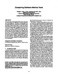
(c) Moving mean

Fig. 2: Example effect of data transformations. The y-axis represents the percentage of code in the very-high risk category and the x-axis represents 15 systems of the benchmark.

E. Data transformations One potential threat to validity in our approach is the risk of over-fitting a particular set of systems. Namely, the specific thresholds obtained can be conditioned by particular discontinuities in the data. In order to reduce that effect, one can apply smoothing transformations to each risk category where thresholds are picked out from. We experimented with two transformations: (i) interpolation, in which each data point is replaced by the interpolation of its value and the consecutive one, and (ii) moving mean, in which each data point is replaced by the mean of a window of points around it (this example used a 2-points window). The effect of each transformation is shown in Figure 2, using a part of the Very-high risk category for the Module Inward Coupling metric where a discontinuity can be observed in the raw data. Other transformations could be used and easily add to the algorithm. In practice, due to the large number of data points used, we have not observed a significative difference in the calibrated thresholds. No other issues were observed with the use of thresholds from transformed data. When using a small number of data points (benchmark systems) having many discontinuities, data transformations might be relevant to smooth the data. In theory, this will reduce the risk of over-fitting a particular set of systems and keep the traceability capabilities. However, the implications of this approach are still open for research. V. A PPLICATION We have successfully applied the methodology to calibrate rating thresholds for all metrics of the SIG Quality Model [6] using an industry based benchmark. In this section, we will describe the benchmark and discuss the calibrated thresholds. A. Benchmark For ratings calibration we have used the same industrybased benchmark as in [8]. This was done because the methodologies presented in [8] and this paper are related, and to be able to use the same 1st-level thresholds. The benchmark used to derive risk thresholds and calibrate rating thresholds is made of both proprietary and open-source systems, implemented in modern object-oriented languages, C# and Java. A total of 100 systems were used, with sizes ranging from 3K to nearly 800K LOC in a total of almost 12 million LOC, being representative of different application

TABLE I: Systems per technology and license. Technology Java C#

License

n

LOC

Proprietary OSS Proprietary OSS Total

60 22 17 1 100

8,435K 2,756K 794K 10K 11,996K

TABLE III: Risk and rating thresholds for the SIG Quality Model metrics. The risk thresholds are defined in the headers, and the rating thresholds are defined in the table body. (a) Unit Size metric (LOC at method level). Star rating ★★★★★ ★★★★✩ ★★★✩✩ ★★✩✩✩

TABLE II: Systems per functionality. Functionality type

n

Catalogue or register of things or events Customer billing or relationship management Document management Electronic data interchange Financial transaction processing and accounting Geographic or spatial information systems Graphics and publishing tools or system Embedded software for machine control Job, case, incident or project management Logistic or supply planning and control Management or performance reporting Mathematical modeling (finance or engineering) Online analysis and reporting Operating systems or software utility Software development tool Stock control and order processing Trading Workflow support and management Other Total

8 5 5 3 12 2 2 3 6 8 2 1 6 14 3 1 1 10 8 100

domains. Table I provides a breakdown of the number of systems and LOC for technology and license. Table II provides a characterization of the systems according to its functionality as defined by ISBSG in [12].

Low risk ]0, 30] -

High risk ]44, 74] 10.9 15.5 22.2 31.4

Very-high risk ]74, ∞[ 3.9 6.5 11.0 18.1

(b) Unit Complexity metric (McCabe at method level). Star rating ★★★★★ ★★★★✩ ★★★✩✩ ★★✩✩✩

Low risk ]0, 6] -

Moderate risk ]6, 8] 17.9 23.4 31.3 39.1

High risk ]8, 14] 9.9 16.9 23.8 29.8

Very-high risk ]14, ∞[ 3.3 6.7 10.6 16.7

(c) Unit Interfacing metric (Number of parameters at method level). Star rating ★★★★★ ★★★★✩ ★★★✩✩ ★★✩✩✩

Low risk [0, 2] -

Moderate risk [2, 3[ 12.1 14.9 17.7 25.2

High risk [3, 4[ 5.4 7.2 10.2 15.3

Very-high risk [4, ∞[ 2.2 3.1 4.8 7.1

(d) Module Inward Coupling metric (Fan-in at file level). Star rating ★★★★★ ★★★★✩ ★★★✩✩ ★★✩✩✩

Low risk [0, 10] -

Moderate risk [10, 22[ 23.9 31.2 34.5 41.8

High risk [22, 56[ 12.8 20.3 22.5 30.6

Very-high risk [56, ∞[ 6.4 9.3 11.9 19.6

no deviations.

B. Rating thresholds for the SIG Quality Model metrics We have applied the methodology to calibrate ratings for all metrics from the SIG Quality Model [6]: unit complexity (McCabe at method level), unit size (LOC at method level), unit interfacing (number of parameters at method level) and module inward coupling (fan-in at file level). Table III presents both the 1st-level thresholds derived with the methodology previously introduced by the authors [8] and the 2nd-level thresholds, or rating thresholds, calibrated with the algorithm presented in this paper. The metric thresholds for the unit complexity were previously presented in Section II. As we can observe, all the thresholds are monotonic between risk categories and ratings, i.e., the thresholds become more lenient from high to lower risk categories and from higher to lower ratings. Also, for all metrics, there are no repeated thresholds. This indicates, that our methodology was successful in differentiating the systems of the benchmark and consequently deriving good rating thresholds. For all the metrics, we used the rating thresholds calibrated from the benchmark, to rate all benchmark systems. This was done to verify if the expected distribution, 20–20–20-20–20, was in fact met by the calibration algorithm. For all metrics we verified that the expected distribution was achieved with

Moderate risk ]30, 44] 19.5 26.0 34.1 45.9

VI. S TABILITY ANALYSIS In order to assess the reliability of the thresholds obtained, we performed a stability analysis. The general approach is to run the calibration algorithm n times, each with a randomly sampled subset of the systems present in the original set. The result is n threshold tables per metric. Two ways of assessing these numbers are then possible: (i) inspect the variability in the threshold values; (ii) apply the thresholds to the original set of systems and inspect the differences in ratings. Using, again, the benchmark presented in Section V, we performed 100 runs (n = 100), each of those with 90% of the systems (randomly sampled). To assess the stability of the rating thresholds, we calculated, for each threshold, the absolute relative differences from its median throughout all the runs5 . This amounts to 12 threshold values per run, thus 100 × 12 = 1200 data points. In Table IV we present for individual metrics the obtained threshold ranges and in Table V we present summary statistics as percentages. Looking at Table V we observe that all properties exhibit a very stable behavior, with 75% 5 Thus, for a threshold t (calculated in run number i ∈ [1, n[) one has i |t −median(t )| δti = i median(t )n . n

TABLE IV: Variability of the rating thresholds for 100 runs, randomly sampling 90% of the systems in the benchmark. (a) Unit Size metric. Star rating ★★★★★ ★★★★✩ ★★★✩✩ ★★✩✩✩

Moderate risk 18.5 - 20.6 24.6 - 28.2 33.5 - 35.9 43.2 - 46.4

High risk 8.9 - 11.1 14.4 - 18.0 21.1 - 26.0 30.0 - 33.3

Very-high risk 3.7 - 3.9 5.8 - 7.8 10.0 - 12.7 17.3 - 19.5

(b) Unit Complexity metric. Star rating ★★★★★ ★★★★✩ ★★★✩✩ ★★✩✩✩

Moderate risk 17.3 - 20.0 23.5 - 25.5 29.5 - 32.9 35.9 - 40.9

Star rating ★★★★★ ★★★★✩ ★★★✩✩ ★★✩✩✩

Moderate risk 11.1 - 13.0 14.8 - 15.7 17.2 - 21.2 25.2 - 27.6

High risk 9.8 - 12.3 16.1 - 18.9 20.8 - 24.8 28.0 - 30.8

VII. R ELATED WORK

Very-high risk 3.2 - 4.2 6.2 - 8.5 9.7 - 12.6 14.5 - 17.1

Various alternatives for aggregating measurements have been proposed: addition, central tendency measures, distribution parameter fitting, wealth inequality measures or custom formulae. In this section, we discuss these alternatives and compare them to our approach.

(c) Unit Interfacing metric. High risk 4.7 - 5.7 6.9 - 7.6 8.3 - 10.2 12.8 - 18.0

Very-high risk 2.0 - 2.3 2.8 - 3.5 4.5 - 5.0 6.1 - 7.1

A. Addition

(d) Module Inward Coupling metric. Star rating ★★★★★ ★★★★✩ ★★★✩✩ ★★✩✩✩

Moderate risk 23.0 - 26.0 29.3 - 31.6 34.5 - 36.9 41.5 - 48.7

High risk 12.8 - 15.1 18.6 - 20.7 21.9 - 23.7 28.9 - 36.4

Very-high risk 5.7 - 7.4 8.4 - 10.0 10.1 - 13.3 15.1 - 20.7

TABLE V: Summary statistics on the stability of rating thresholds.

Unit size Unit complexity Unit interfacing Module coupling

Q1 0.0 0.0 0.0 0.0

Median 0.4 0.3 0.0 0.0

Q3 3.2 4.4 5.5 5.3

95% 10.7 11.7 14.1 18.0

Max 23.8 27.3 25.9 23.4

µ 2.6 3.2 3.3 3.3

TABLE VI: Summary statistics on stability of the computed ratings.

Unit size Unit complexity Unit interfacing Module coupling

Q1 0.0 0.0 0.0 0.0

Median 0.3 0.3 0.4 0.4

Q3 1.0 1.5 1.5 1.4

95% 3.5 4.3 5.1 5.9

Max 7.9 9.7 12.1 14.3

We observe that the model is more stable at the ratings level than at the threshold level. This is to be expected since differences in thresholds of different risk categories for the same rating can compensate each other. We can conclude that there is limited impact to the ratings caused by including or excluding specific systems or small groups of systems. This indicates good stability of the results obtained using this benchmark.

µ 0.8 1.0 1.1 1.2

of the data points (Q3 ) deviating less than 6% from the medians. There are some extreme values, the largest one being a 27.3% deviation in Unit complexity. Nevertheless, even taking into account the full range, thresholds were observed to never overlap and maintain their strictly monotonous behavior, which increases our confidence in both the method and the calibration set. In order to assess the stability of the threshold values in terms of the computed ratings, we calculated, for each system, the absolute differences from its median rating throughout all the runs. This amounts to 100 × 100 = 10000 data points. In Table VI we present summary statistics on the results, made relative to the possible range of 5.5 − 0.5 = 5 (shown as percentages). Again, all properties exhibit a very stable behavior, with 75% of the data points (Q3 ) deviating less than 1.6% from the medians.

One of the most basic ways of aggregating measurements is to use addition. Individual measurements are all added together and the total is reported at system level. Lanza and Marinescu [13] use addition to aggregate the NOM (Number of Operations) and CYCLO (McCabe cyclomatic number) metrics at system-level. Chidamber and Kemerer [3] use addition to aggregate the individual complexity numbers of methods into the WMC (Weighted Methods per Class) metric at class level. When adding measurements together we lose information about how these measurements are distributed in the code which precludes pinpointing potential problems. For example, the WMC metric does not distinguish between a class with many methods of moderate size and complexity and a class with a single huge and highly complex method. In our methodology, the risk profiles and the mappings to ratings ensure that such differences in distribution are reflected in the system-level ratings. B. Central tendency Central tendency functions such as mean (simple, weighted or geometric) or the median have also been used to aggregate metrics by many authors. For example, Spinellis [14] aggregates metrics at system level using the mean and the median, and uses these values to perform comparisons between four different operating-system kernels. Coleman et al. [15], in the Maintainability Index model, aggregate measurements at system-level using the mean. The simple mean directly inherits the drawbacks of aggregation by addition, since the mean is calculated as the sum of measurements divided by their number. In general, central tendency functions fail to do justice to the skewed nature of most software-related metrics. Many authors have shown that software metrics are heavily skewed [3], [4], [1], [16], [17] providing evidence that metrics should be aggregated using other techniques. Spinellis [14] provided additional evidence that central tendency measures should not be used to aggregate measurements as he concluded that it was not possible to clearly differentiate the studied systems.

The skewed nature of source code metrics is accommodated by the use of risk profiles in our methodology. The derivation of thresholds from benchmark data ensure that differences in skewness among systems are captured well at the first level [8]. In the calibration of the mappings to ratings at the second level, the ranking of the systems is also based on their performance against the thresholds, rather than on a central tendency measure, which ensures that the ranking adequately takes the differences between systems in the tails of the distributions into account. C. Distribution fitting A common statistical methodology to describe data is to fit it against a particular distribution. This involves the estimation of distribution parameters and quantification of goodness of fit. These parameters can then be used to characterize the distribution data. Hence, fitting a distribution parameter can be seen as a methodology to aggregate measurements at system-level. For instance, Concas et al. [1], Wheeldon and Counsell [16] and Louridas et al. [17] have shown that several metrics follow power-law or log-normal distributions, computing the distribution parameters for a set of systems as case study. This approach has several drawbacks. First, the assumption that for all systems a metric follows the same distribution (albeit with different parameters) may be wrong. In fact, when a group of developers starts to act on the measurements for the code they are developing, the distribution of that metric may rapidly change into a different shape. As a result, the assumed statistical model no longer holds and the distribution parameters stop to be meaningful. Secondly, to understand the characterization of a system by its distribution parameters requires software engineering practitioners to understand the assumed statistical model, which undermines the understandability of this aggregation method. Also, root-cause analysis, i.e., tracing distribution parameters back to problems at particular source code locations, is not straightforward. Our methodology does not assume a particular statistical model, and could therefore be described as non-parametric. This makes it robust against lack of conformance to such a model by particular systems, for instance due to quality feedback mechanisms in development environments and processes. D. Wealth inequality Aggregation of software metrics has also been proposed using the Gini coefficient by Vasa et al. [4] and the Theil index by Serebrenik and Van den Brand [5]. The Gini coefficient and the Theil index are used in economics to quantify the inequality of wealth. An inequality value of 0 means that measurements follow a constant distribution, i.e., all have the same value. A high value of inequality, on the other hand, indicates a skewed distribution, where some measurements are much higher than the others. Both Gini and Theil adequately deal with the skewness of source code metrics without making assumptions about an underlying distribution. Both have shown good results when

applied to software evolution analysis and to detect automatically generated code. Still they suffer of major shortcomings when used to aggregate source code measurement data. Firstly, both Gini and Theil provide indications of the differences in quality of source code elements within a system, not of the degree of quality itself. This can easily be seen from an example. Let us assume that for a class-level metric M , higher values indicate poorer quality. Then, let’s assume that a system A has three equally-sized classes with metric values 1, 1 and 100 (Gini=0.65 and Theil=0.99), and that a system B also has three equally-sized classes with values 1, 100 and 100 (Gini=0.33 and Theil=0.38). Clearly, system A has higher quality, since one third rather than two thirds of its code suffers from poor quality. But both Gini and Theil indicate that A has greater inequality, making it score lower than B. Thus, even though inequality in quality may often indicate low quality, they are conceptually different. Secondly, these aggregation techniques do not allow rootcause analysis, i.e., they do not provide means to identify the underlying measurements which explain the computed inequality. The Theil index, which improves over the Gini factor, provides means to explain the inequality according to a specific partition by reporting a value for how much a specific partition of measurements accounts for the overall inequality. However, Theil is limited to provide insight at the partition level not providing information at lower levels. Similarly to the Gini coefficient and the Theil index, the ratings based on risk-profile that we propose capture differences between systems that occur when quality values are distributed unevenly over source code elements. But by contrast, our method is also based on the magnitude of the metric values rather than exclusively on the inequality among them. E. Custom formula Jansen [18] proposed the confidence factor as a metric to aggregate violations reported by static code checkers. The confidence factor is derived by a formula taking into account the total number of rules, the number of violations, the severity of violations and the overall size of the system, and the percentage of files that are successfully checked, reporting a value between 0 and 100. The higher the value the higher the confidence on the system. A value of 80 is normally set as minimum threshold. Although the author reports the usefulness of the metric, he states that the formula definition is based on heuristics and requires formal foundation and validation. Also, root-cause analysis can only be achieved by investigating the extremal values of underlying measurements. In contrast we proposed a methodology to derive thresholds from benchmark data which can be used both to aggregate measurements into ratings and to trace back the ratings back to measurements. VIII. C ONCLUSION AND F UTURE W ORK We presented a methodology for the calibration of mappings from code-level measurements to system-level ratings. Calibration is done against a benchmark of software systems and

their associated code measurements. The presented methodology complements our earlier work on deriving thresholds for source code metrics from such benchmark data [8]. The core of our methodology is an iterative algorithm that (i) ranks systems by their performance against pre-determined thresholds and (ii) based on the obtained ranking determines how performance against the thresholds translates into ratings on a unit-less scale. The contributions of the paper are: • • • • •

An algorithm to perform calibration of thresholds for quality profiles; Formalization of the calculation of ratings from quality profiles; Discussion of the caveats and options to consider when using our approach; An application of the methodology to determine thresholds for 4 source code metrics; A procedure to assess the stability of the thresholds obtained with a particular data set.

The extended methodology is a generic blueprint for building metrics-based quality models. As such, it can be applied to any situation where one would like to perform automatic qualitative assessments based on multi-dimensional quantitative data. The presence of a large, well-curated repository of benchmark data is, nevertheless, a prerequisite for successful application of our methodology. Other than that, one can imagine applying it to assess software product quality but using a different set of metrics, assessing software process or software development community quality, or even applying it to areas outside software development. The methodology is applied by SIG to annually re-calibrate the SIG quality model [6], [7], which forms the basis of the evaluation and certification of software maintainability ¨ conducted by SIG and TUViT [19]. A. Future work In the current paper we have applied the methodology to particular metrics. We want to systematically explore the application to a much wider range of metrics in order to investigate the limits of generalizability. For example, we have started applying the methodology for metrics concerning test quality, issue handling efficiency, library usages, and more. In the SIG quality model, a 5-star rating scale has been calibrated against a 5-30-30-30-5 percentile distribution. We want to investigate further what the implications are of using a scale with a different number of quality levels and a different percentile distribution. The sensitivity analysis that we presented allows quantification of the influence of the composition and size of the benchmark repository on the calibration results. This helps for instance to assist in guarding the volatility of thresholds and mappings when re-calibrating. We would like to elaborate this sensitivity analysis further into a structured procedure for deciding the adequacy of a benchmark repository. Finally, we would like to combine the methodology presented in this paper with ongoing work on methods for metric

selection, metric data collection, and metric validation, into a comprehensive methodology for quality model construction. ACKNOWLEDGMENTS Thanks to Paulo F. Silva for providing comments to earlier versions of this work. The first author is supported by the Fundac¸a˜ o para a Ciˆencia e a Tecnologia (FCT), grant SFRH/ BD/30215/2006, and SSaaPP project, FCT contract no. PTDC/ EIA-CCO/108613/2008. R EFERENCES [1] G. Concas, M. Marchesi, S. Pinna, and N. Serra, “Power-laws in a large object-oriented software system,” IEEE Trans. Softw. Eng., vol. 33, no. 10, pp. 687–708, 2007. [2] T. J. McCabe, “A complexity measure,” Software Engineering, IEEE Transactions on, vol. SE-2, no. 4, pp. 308–320, Dec. 1976. [3] S. R. Chidamber and C. F. Kemerer, “A metrics suite for object oriented design,” IEEE Trans. Softw. Eng., vol. 20, no. 6, pp. 476–493, 1994. [4] R. Vasa, M. Lumpe, P. Branch, and O. Nierstrasz, “Comparative analysis of evolving software systems using the Gini coefficient,” ICSM’09, pp. 179–188, 2009. [5] A. Serebrenik and M. van den Brand, “Theil Index for aggregation of software metrics values,” ICSM’10, 2010. [6] I. Heitlager, T. Kuipers, and J. Visser, “A practical model for measuring maintainability,” International Conference on the Quality of Information and Communications Technology (QUATIC’07), pp. 30–39, 2007. [7] J. P. Correia and J. Visser, “Certification of technical quality of software products,” in Proc. of the Int’l Workshop on Foundations and Techniques for Open Source Software Certification, 2008, pp. 35–51. [8] T. L. Alves, C. Ypma, and J. Visser, “Deriving metric thresholds from benchmark data,” ICSM’10, pp. 1–10, 2010. [9] ISO/IEC, “IS 80000–2:2009: Quantities and units — part 2: Mathematical signs and symbols to be used in the natural sciences and technology,” International Organization for Standardization, Geneva, Switzerland., Tech. Rep., December 2009. [10] R. Likert, “A technique for the measurement of attitudes,” Archives of Psychology, vol. 22, no. 140, pp. 1 – 55, 1932. [11] R. Baggen, K. Schill, and J. Visser, “Standardized code quality benchmarking for improving software maintainability,” in Proc. of the Int’l Workshop on Software Quality and Maintainability, 2010. [12] C. Lokan, “The Benchmark Release 10 - project planning edition,” International Software Benchmarcking Standards Groups Ltd., Tech. Rep., February 2008. [13] M. Lanza and R. Marinescu, Object-Oriented Metrics in Practice. Using Software Metrics to Characterize, Evaluate, and Improve the Design of Object-oriented Systems. Springer Verlag, 2010. [14] D. Spinellis, “A tale of four kernels,” in ICSE’08. New York, NY, USA: ACM, 2008, pp. 381–390. [15] D. Coleman, B. Lowther, and P. Oman, “The application of software maintainability models in industrial software systems,” J. Syst. Softw., vol. 29, no. 1, pp. 3–16, 1995. [16] R. Wheeldon and S. Counsell, “Power law distributions in class relationships,” SCAM’03, vol. 0, p. 45, 2003. [17] P. Louridas, D. Spinellis, and V. Vlachos, “Power laws in software,” TOSEM’08, vol. 18, no. 1, Sep 2008. [18] P. Jansen, “Turning static code violations into management data,” Working Session on Industrial Realities of Program Comprehension (IRPC) at the 16th IEEE Int. Conf. on Program Comprehension (ICPC’08), 2008. [19] R. Baggen, J. P. Correia, K. Schill, and J. Visser, “Standardized code quality benchmarking for improving software maintainability,” Software Quality Journal, pp. 1–21, 2011.