Jul 14, 2015 - Girkmann benchmark problem involving a spherical shell stiffened with a foot ring. ... to this document may be directed to that email address. 1 ...
Downloaded 08/18/16 to 130.231.240.17. Redistribution subject to SIAM license or copyright; see http://www.siam.org/journals/ojsa.php
SIAM J. SCI. COMPUT. Vol. 38, No. 3, pp. B440–B457
c 2016 Society for Industrial and Applied Mathematics �
BENCHMARK COMPUTATIONS OF STRESSES IN A SPHERICAL DOME WITH SHELL FINITE ELEMENTS∗ ANTTI H. NIEMI† Abstract. We present a computational framework for analyzing thin shell structures using the finite element method. The framework is based on a mesh-dependent shell model which we derive from the general laws of three-dimensional elasticity. We apply the framework for the so-called Girkmann benchmark problem involving a spherical shell stiffened with a foot ring. In particular, we compare the accuracy of different reduced strain four-node elements in this context. We conclude that the performance of the bilinear shell finite elements depends on the mesh quality but reasonable accuracy of the quantities of interest of the Girkmann problem can be attained in contrast to earlier results obtained with general shell elements for the problem. Key words. shell structures, finite elements, thin shell theory, convergence, stabilized methods, locking AMS subject classifications. 65N30, 74S05, 74K25 DOI. 10.1137/15M1027590
1. Introduction. The role of thin shell theory in structural analysis has changed dramatically over centuries from center stage to supporting cast, partly because of the advent of the finite element method. This paper will bring shell theory back to the forefront by studying a family of four-node finite elements based on it. The study is carried out in the context of a challenging benchmark problem involving a stiffened doubly curved thin shell. Conventional shell finite element formulations involve various explicit and implicit modeling assumptions that extend beyond the limits of mathematical convergence theory currently available. The theoretical problems arise from the fact that the general shell elements used in industrial finite element analysis have been developed through “finite element modeling,” where the connection of the discretization to the actual differential operators of the mathematical shell model is obscure; cf. [31]. A prerequisite for traditional finite element error analysis is a well-posed variational problem formulated in some suitable Hilbert space. For shells such mathematical models can be formulated using differential geometry of surfaces and theoretically stable formulations have been analyzed, e.g., in [24, 1, 6]. However, these works deal only with the bending-dominated deformations and do not address the membranedominated and intermediate cases which are very important for instance in civil and structural engineering. We refer the reader to [29] for a precise characterization of different shell deformation states in context of cylindrical shells. On the other hand, it is possible to interpret the modeling assumptions of conventional shell elements in context of the mathematical models. For instance, the degenerated solid approach associated to certain four-node elements has been translated to explicit strain reduction procedure within a specific shell model in [17, 18] and ∗ Submitted to the journal’s Computational Methods in Science and Engineering section June 23, 2015; accepted for publication (in revised form) April 4, 2016; published electronically June 21, 2016. This work was supported by the Academy of Finland through the project How to Handle the Prima Donna of Structures: Analysis and Development of Advanced Discretization Techniques for the Simulation of Thin Shells (260302). http://www.siam.org/journals/sisc/38-3/M102759.html † Aalto University, Espoo, 00076 Finland (antti.h.niemi@aalto.fi).
B440
Copyright © by SIAM. Unauthorized reproduction of this article is prohibited.
Downloaded 08/18/16 to 130.231.240.17. Redistribution subject to SIAM license or copyright; see http://www.siam.org/journals/ojsa.php
BENCHMARK COMPUTATIONS OF STRESSES IN A DOME
B441
that procedure has been numerically analysed in [11, 12, 22, 19]. This line of research is not limited to the theoretical analysis of existing formulations only. It can also be used to enhance the formulations and develop new ones as shown in [20], where a new four-node shell finite element of arbitrary quadrilateral shape was developed based on shell theory. Thanks to modern computation technology, such as the hp-adaptive finite element method [7, 34], shell analysis can also be based directly to three-dimensional elasticity theory. Such an approach rules out the modeling errors arising from the simplifications of dimensionally reduced structural models but requires more degrees of freedom for the discrete model. Also, if simplified representations of the stress state such as the stress resultants are needed, they must be post-processed from the three-dimensional stress field, and this can be nontrivial. A model problem called the Girkmann problem, which was revived some time ago, highlights the above complications rather dramatically; see [32, 21, 28, 8]. The problem involves a concrete structure consisting of a spherical dome stiffened by a foot ring under a dead gravity load. The task is to determine the values of the shear force and the bending moment at the junction between the dome and the ring as well as the maximum bending moment in the dome. The problem was initially presented and solved analytically in the textbook [10]. More recently, in the bulletin of the International Association of Computational Mechanics (IACM) [26], the problem was posed as a computational challenge to the finite element community. The purpose of the challenge was to find out how the process of verification, that is, the process of building confidence that an approximative result is within a given tolerance of the exact solution to the mathematical model, is carried out by the community given the Girkmann problem. The results have been summarized in [27, 32] without attribution and details on how verification was actually performed. Out of the 15 results submitted, 11 have a very large dispersion and are not within any acceptable tolerance of the reference values computed in [32, 21, 28] using different models and formulations. So far detailed verification studies have been published for the axisymmetric models based on elasticity theory as well as axisymmetric dimensionally reduced models. In [32], the p-version of the finite element method was used in conjunction with the extraction procedure of [3] to compute accurate values for the quantities of interest. Similar approach with the hp-version of the finite element method was taken in [21], where also the axisymmetric h-version with selective reduced integration was successfully employed to discretize the dimensionally reduced model. In the present work, we introduce a finite element framework for thin shell analysis and use the Girkmann problem to demonstrate its possibilities. More precisely, we benchmark different variants of the MITC-type shell element proposed earlier by the author in [20] by modeling a quarter of the dome and by using symmetry boundary conditions. We show that the performance of the formulations varies depending on the performed strain reductions and the mesh regularity. Nevertheless, reasonable accuracy for the main quantities of interest is obtained contrary to the earlier published results obtained with general shell elements. The main difference of the present approach as compared with the conventional ones is that the quadrilateral mesh is not taken as such to represent the shell middle surface. Rather, it serves only as a computational domain used to represent the imagined shell middle surface by interpolating the nodal normal vector. The paper is organized as follows. In the next section, we develop the shell theory used to construct the different finite element methods. The finite element methods
Copyright © by SIAM. Unauthorized reproduction of this article is prohibited.
Downloaded 08/18/16 to 130.231.240.17. Redistribution subject to SIAM license or copyright; see http://www.siam.org/journals/ojsa.php
B442
ANTTI H. NIEMI
are described in section 3 together with a discussion on their well-posedness and implementation aspects. Section 4 is devoted to description of the analysis procedure for the Girkmann problem and numerical results. The paper ends with conclusions in section 5. 2. Variational formulation of the shell problem. We will employ the Einstein summation convention so that Greek indices range over the values 1, 2 while Latin indices have the values 1, 2, 3. The former refer to surface coordinates while the latter refer to general three-dimensional curvilinear coordinates. Our surface coordinate systems can be assumed orthonormal so that we can formulate our straindisplacement relations and constitutive laws directly in terms of physical components and traditional partial derivatives, which will be denoted by a comma. Moreover, Euclidean vectors are displayed using overhead arrows, whereas boldface notation is reserved for the column vectors and matrices storing the components of different surface tensors in the assumed orthonormal coordinate system. A shell domain Ω ⊂ R3 of constant thickness t is defined as (2.1)
� Ω = Φ(K × (−t/2, t/2)),
� is of the form where the shell mapping Φ (2.2)
� Φ(x, y, ζ) = �r(x, y) + ζ�n(x, y).
Here the parametric surface �r(x, y) represents the middle surface of the shell and �n(x, y) is the unit normal vector to the middle surface. Thus ξ1 = x, ξ2 = y, and ξ3 = ζ constitute a curvilinear coordinate system in 3-space, called shell coordinates. In the following, we imagine that the middle surface is defined as (2.3)
�r(x, y) = x�i1 + y�i2 + f (x, y)�i3 ,
(x, y) ∈ K,
where �i1 ,�i2 ,�i3 are fixed Cartesian unit vectors. Moreover, we assume that the middle surface differs only little from the coordinate plane K, i.e., the shell is shallow. More precisely, we assume that the function f : K → R is smooth in the curvature length scale R defined by 1 = max ||f,αβ ||∞,K . α,β R If hK = diam(K) and R is taken as the length unit, the shallowness assumption can be formulated as (2.4)
ˆ K ), f,α = O(h
ˆ K = hK /R ≤ 1. where h Under the shallowness assumption (2.4), the tangent basis vectors (2.5)
�eα (x, y) = �iα + f,α (x, y)�i3
associated to the middle surface parametrization (2.3) are orthonormal within the ˆ 2 ). accuracy of O(h K 2.1. Shell kinematics. According to the standard kinematic hypothesis we assume that the displacement vector can be written in the form (2.6)
� (x, y, ζ) = (uλ (x, y) + ζθλ (x, y))�eλ (x, y) + w(x, y)�n(x, y), U
Copyright © by SIAM. Unauthorized reproduction of this article is prohibited.
Downloaded 08/18/16 to 130.231.240.17. Redistribution subject to SIAM license or copyright; see http://www.siam.org/journals/ojsa.php
BENCHMARK COMPUTATIONS OF STRESSES IN A DOME
B443
where u = (u1 , u2 ) are the tangential displacements of the middle surface, w is the transverse deflection, and the quantities θ = (θ1 , θ2 ) are the angles of rotation of straight material fibres normal to the middle surface. Referring to the curvilinear coordinates ξ1 = x, ξ2 = y, and ξ3 = ζ, the linearized Green–Lagrange strain tensor is defined by eij =
(2.7)
1 � � ,j + Φ � ,j · U � ,i ), (Φ,i · U 2
i, j = 1, 2, 3.
We find directly from (2.6) that (2.8)
� ,α = (uλ,α + ξ3 θλ,α )�eλ + (uλ + ξ3 θλ )�eλ,α + w,α�n + w�n,α U
for α = 1, 2 and � ,3 = θλ�eλ . U
(2.9)
Similarly, the combination of (2.2), (2.3), and (2.5) yields � ,α = �eα + ζ�n,α , Φ
(2.10)
α = 1, 2,
and � ,3 = �n. Φ
(2.11)
The components of the strain tensor are represented as a power series of the variable ζ. If we take into account two terms, the in-plane strains may be written as eαβ ≈ εαβ + ζκαβ .
(2.12)
Using relations (2.10) and (2.8), the membrane strain tensor εαβ = eαβ |ζ=0 , which arises from stretching of the deformed middle surface, can be written as εαβ ≈
(2.13)
1 (uα,β + uβ,α ) − bαβ w, 2
where f,αβ bαβ = −�eα · �n,β = � , 1 + f,λ f,λ
(2.14)
α, β = 1, 2,
are the coefficients of the second fundamental form of the middle surface. In (2.13), terms multiplied by the “rotation coefficients” �eα · �eλ,β have been neglected as quanˆ K ) based on the shallowness assumption (2.4). We content tities of relative order O(h ourselves here to first order of accuracy since, in general, the coefficients bαβ cannot be approximated more precisely with linear or bilinear interpolation functions; see section 3.3. Introducing the coefficients of the third fundamental form of the middle surface cαβ = �n,α · �n,β ,
α, β = 1, 2,
∂e
the elastic curvature tensor καβ = ∂ζαβ |ζ=0 in (2.12), which arises from bending of the deformed middle surface, comes out as (2.15)
καβ ≈
1 1 (θα,β + θβ,α ) + cαβ w − (bαλ uλ,β + bβλ uλ,α ), 2 2
α, β = 1, 2
Copyright © by SIAM. Unauthorized reproduction of this article is prohibited.
Downloaded 08/18/16 to 130.231.240.17. Redistribution subject to SIAM license or copyright; see http://www.siam.org/journals/ojsa.php
B444
ANTTI H. NIEMI
based again directly on (2.10) and (2.8). Here, terms multiplied by �eα ·�eλ,β or �n,α ·�eλ,β ˆ K ). have been neglected as quantities of relative order O(h It is possible to simplify the bending strain expressions by sacrificing their tensorial invariance. It is straightforward to verify that cαβ ≈ bαλ bλβ within the adopted accuracy, so that we may write (2.15) componentwise as κ11 ≈ θ1,1 + b12 (b12 w − u2,1 ) − b11 ε11 , (2.16)
κ22 ≈ θ2,2 + b12 (b12 w − u1,2 ) − b22 ε22 , κ12 ≈
1 b12 (θ1,2 + θ2,1 + b11 (b12 w − u1,2 ) + b22 (b12 w − u2,1 )) − (ε11 + ε22 ). 2 2
In these expressions, the contribution of the terms b11 ε11 , b22 ε22 , and b12 (ε11 + ε22 ) to the maximum in-plane strains at the outer and inner surfaces of the shell is of relative order O(t/R) only. Therefore, the number of terms in the kinematic relations can be slightly reduced by retaining only the underlined terms in the calculations. Finally, the transverse shear strains are defined as γα = 2eα3 ,
(2.17)
α = 1, 2.
These can be written in terms of the displacements by first noting that since �eα and �n are orthogonal, we have �eα,β · �n = −�eα · �n,β , and consequently bαβ = �n · �eα,β . Now, the combination of (2.11) with (2.8) and (2.10) with (2.9) according to (2.7) yields (2.18)
γα = θα + bλα uλ + w,α ,
α = 1, 2,
and completes the description of shell kinematics. 2.2. Constitutive equations. Assuming linearly elastic isotropic material with Poisson ratio ν and Young modulus E, the constitutive law relating stresses and strains can be written with respect to the approximately orthogonal shell coordinate system (x, y, ζ) attached to the middle surface as E [(1 − ν)eαβ + νeλλ δαβ ] , 1 − ν2 E eα3 , α, β = 1, 2, = 1+ν
σαβ = (2.19) σα3
where δαβ is the Kronecker delta. The elastic coefficients in the above formula have been modified to yield so-called plane stress state tangent to the middle surface. This modification is necessary to avoid Poisson locking in context of the kinematic assumption (2.6). We follow the standard convention of structural mechanics and introduce the internal forces and moments which are the stress resultants and stress couples per unit length of the middle surface. These can now be defined as � t/2 � t/2 � t/2 (2.20) σαβ dζ, mαβ = σαβ ζ dζ, qα = σα3 dζ nαβ = −t/2
−t/2
−t/2
and correspond to the membrane forces, bending moments, and transverse shear forces in static equilibrium considerations.
Copyright © by SIAM. Unauthorized reproduction of this article is prohibited.
Downloaded 08/18/16 to 130.231.240.17. Redistribution subject to SIAM license or copyright; see http://www.siam.org/journals/ojsa.php
BENCHMARK COMPUTATIONS OF STRESSES IN A DOME
B445
2.3. Potential energy functional. Integrals over the shell domain Ω can be evaluated in terms of the assumed shell coordinates as � � � t/2 {·} dΩ ≈ {·} dζdxdy. Ω
K
−t/2
The combination of (2.20), (2.19), (2.17), and (2.12) allows us to write the elastic strain energy functional as � 1 (σαβ eαβ + σα3 eα3 ) dΩ UK (u, w, θ) = 2 Ω � (2.21) 1 ≈ (nαβ εαβ + qα γα + mαβ καβ ) dxdy, 2 K where Et [(1 − ν)εαβ + νελλ δαβ ] , 1 − ν2 Et qα = γα , 2(1 + ν) Et3 [(1 − ν)καβ + νκλλ δαβ ] mαβ = 12(1 − ν 2 ) nαβ =
(2.22)
and the strains are given in terms of the displacements in (2.13), (2.18), and (2.16). Similarly, the potential energy corresponding to external distributed surface forces (f1 , f2 , p) and moments (τ1 , τ2 ) as well as edge forces (N1 , N2 , Q) and moments (M1 , M2 ) is � VK (u, w, θ) = − (fλ uλ + pw + τλ θλ ) dxdy �K (2.23) − (Nλ uλ + Qw + Mλ θλ ) ds, ∂K
and the total energy is given by the sum (2.24)
EK (u, w, θ) = UK (u, w, θ) + VK (u, w, θ).
˜ is 3. Finite element methods. We assume that the whole shell domain Ω formed as the union � ˜= Ω ΩK , K∈Ch
where each ΩK is a domain of the form (2.1) and Ch stands for a mesh of convex quadrilaterals K corresponding to parametrizations of patches of the shell middle surface according to (2.3). We also assume that the whole middle surface � S= �rK (K) K∈Ch
is a smooth surface and that it can be described alternatively by a single, global parametrization ρ �(ξ˜1 , ξ˜2 ). It follows that the transformations between the local and −1 global coordinate systems TK = �rK ◦ρ �, K ∈ Ch , are diffeomorphisms.
Copyright © by SIAM. Unauthorized reproduction of this article is prohibited.
Downloaded 08/18/16 to 130.231.240.17. Redistribution subject to SIAM license or copyright; see http://www.siam.org/journals/ojsa.php
B446
ANTTI H. NIEMI
Without losing generality, we may assume that the coordinates ξ˜1 , ξ˜2 are orthogonal. If {�g1 (ξ˜1 , ξ˜2 ), �g2 (ξ˜1 , ξ˜2 )} are the corresponding normalized tangent vectors of the ˜ and θ˜α stand for the associated displacement and rotation middle surface, and u ˜α , w, K components, then these components are related to the local components uK and α, w K θα as (3.1)
˜λ�gλ · �iα , uK α ◦ TK = u
wK ◦ TK = w, ˜
θαK ◦ TK = θ˜λ�gλ · �iα
according to (2.5) and (2.6). The total potential energy of the structure is expressed as the sum of elementwise contributions such that � ˜ = EK (uK , wK , θK ), (3.2) E(˜ u, w, ˜ θ) K∈Ch
˜ is the globally defined generalized displacement field. The solution where (˜ u, w, ˜ θ) of the problem is determined according to the principle of minimum potential energy from the condition ˜ = min E(˜ ˜ E(˜ u, w, ˜ θ) v , z˜, ψ), ˜ (˜ v ,˜ z ,ψ)∈U
where the energy space U is defined as the set of those kinematically admissible generalized displacement fields for which the energy functional is finite. The existence of a unique minimizer (for maxK hK sufficiently small) follows from the well-posedness of the corresponding Reissner–Naghdi shell model; see, e.g., [5]. It is now straightforward to formulate a finite element method where each displacement component is approximated separately as in the space (3.3)
˜ ∈ U : (uK , wK , θ K ) ∈ [Q1 (K)]5 ∀K ∈ Ch }, Uh = {(˜ u, w, ˜ θ)
where Q1 (K) denotes the standard space of isoparametric bilinear functions on K and (uK , wK , θK ) is the local generalized displacement field defined in (3.1). 3.1. Euler equations. If needed, the system of partial differential equations characterizing the solution of the shell problem can be determined by using calculus of variations. The local form reads −n1λ,λ + b1λ qλ + (b12 m22 ),2 + (b11 m12 ),2 = f1 −n2λ,λ + b2λ qλ + (b12 m11 ),1 + (b22 m12 ),1 = f2 (3.4)
−bαβ nαβ − qλ,λ + (b12 )2 (m11 + m22 ) + (b11 + b22 )b12 m12 = p −m1λ,λ + q1 = τ1 −m2λ,λ + q2 = τ2 .
The first two equations are obtained by calculating the variations of the total energy with respect to the tangential displacements u1 and u2 , and they represent the force balance in the tangential directions �e1 and �e2 , respectively. The third equation corresponds to the force balance in the normal direction �n and is obtained by taking the variation with respect to the transverse deflection w. Finally, variations with respect to the rotations θ1 and θ2 yield the last two equations corresponding to the moment balance about the �e2 and �e1 directions, respectively. Calculus of variations yields also the differential form of the natural boundary conditions. For instance, if K is a rectangle and the boundary coincides with the
Copyright © by SIAM. Unauthorized reproduction of this article is prohibited.
Downloaded 08/18/16 to 130.231.240.17. Redistribution subject to SIAM license or copyright; see http://www.siam.org/journals/ojsa.php
BENCHMARK COMPUTATIONS OF STRESSES IN A DOME
B447
line y = const, the five possible Neumann conditions that complement the separate Dirichlet condition on each displacement component are n12 − b12 m22 − b11 m12 = N1 , n22 = N2 , q2 = Q, m12 = M1 , m22 = M2 . It should be noted that the appearance of the bending moments in the first three balance laws in (3.4) depends on the choice of the expressions for the bending strains. Here, we have used the suggested definition (2.16) that seems to be the simplest one. The ambiguity carries over also to the differential form of the natural boundary conditions and influences the appearance of the effective in-plane shear forces. 3.2. Strain reduction techniques. To avoid locking when approximating bending-dominated problems, membrane and transverse shear strains must be reduced. To introduce the different methods, we denote by F K = (xK , yK ) the bilinear mapping ˆ = [−1, 1] × [−1, 1] onto K and by of the reference square K ⎛ ∂x ∂x ⎞ K
JK
⎜ ∂x ˆ = J K (ˆ x, yˆ) = ⎝ ∂y K ∂x ˆ
K
∂ yˆ ⎟ ∂yK ⎠ ∂ yˆ
ˆ x, yˆ) are the coordinates on K. the Jacobian matrix of F K . Here (ˆ ˆ We start by defining on the reference square K the function spaces
� � y ˆ = sˆ = a + bˆ (3.5) S(K) : a, b, c, d ∈ R c + dˆ x and (3.6)
ˆ = M (K)
� � a + bˆ y c τˆ = : a, b, c, d, e ∈ R c d + eˆ x
for the reduced transverse shear strains and membrane strains, respectively. Denoting ˆ the canonical degrees of freedom associated with by tˆ the unit tangent vector on ∂ K, ˆ S(K) are � ˆ (3.7) sˆ → sˆT tˆdˆ s for every edge eˆ of K, e ˆ
ˆ are defined as whereas the degrees of freedom associated with M (K) � T ˆ τˆ → tˆ τˆtˆdˆ s for every edge eˆ of K, eˆ � (3.8) τˆ → τˆ12 dˆ xdˆ y. ˆ K
The corresponding spaces associated to a general element K ∈ Ch are then defined using covariant transformation formulas as (3.9)
ˆ ˆ) ◦ F −1 s) : sˆ ∈ S(K)} S(K) = {s = (J −T K s K = SK (ˆ
Copyright © by SIAM. Unauthorized reproduction of this article is prohibited.
B448
ANTTI H. NIEMI
Downloaded 08/18/16 to 130.231.240.17. Redistribution subject to SIAM license or copyright; see http://www.siam.org/journals/ojsa.php
and (3.10)
−T ¯ τ ) : τˆ ∈ M (K)}. ˆ ¯−1 τ ◦ F −1 M (K) = {τ = J¯K (ˆ K )J K = MK (ˆ
In case of general quadrilateral elements with nonconstant Jacobian matrices, the transformation in (3.10) must be fixed to a single orientation, e.g., at the midpoint of ˆ so that J¯ = J (0, 0). Otherwise the function space (3.10) for the reduced membrane K strains and stresses does not necessarily include constant fields which would degrade the accuracy of the formulation. ˆ → S(K) ˆ and Π ˆ : H 1 (K) ˆ → M (K) ˆ the interpolation Denoting by ΛKˆ : H 1 (K) K operators associated to the degrees of freedom (3.7) and (3.8), the corresponding projectors for a general K ∈ Ch are defined as ¯K ◦Πˆ ◦M ¯ −1 and ΛK = SK ◦ Λ ˆ ◦ S −1 . ΠK = M K K K K The transformation rule (3.9) guarantees that the degrees of freedom (3.7) are preserved on K: � s → sT t ds for every edge e of K, e
where t is the unit tangent vector on ∂K, but the analogous statement does not hold in context of (3.10) for general meshes. The finite element introduced in (3.5) and (3.7) is a well known edge element denoted by the symbol RTce1 in the recently introduced the periodic table of the finite elements [2] and has been described in the context of plate bending, e.g., in [13, 4]. The element (3.5), (3.8) is less customary at least in the mathematical literature, probably because of its nonelegant extension to quadrilateral shapes. In any case the historical roots of the element are very deep in the literature on finite element technology for plane elasticity. Our current formulation corresponds essentially to the stress field of the Pian–Sumihara element introduced in [23], which in turn may be viewed as an extension of the nonconforming displacement methods introduced by Wilson et. al. [36] and Turner et. al. [35]. We refer the reader to [25] for the complete mathematical theory of these formulations in context of plane elasticity. In the present context, the convergence theory is confined to special cases involving cylindrical or globally shallow shells on special meshes; see [11, 12, 22, 19]. We shall use the label MITC4C for the formulation for which only the transverse shear strains are projected into the space (3.9) (3.11)
γ �→ ΛK γ
and the label MITC4S for the formulation where also the membrane strains are projected: (3.12)
ε �→ ΠK ε,
γ �→ ΛK γ
when evaluating the strain energy according to (2.21) and (2.22). In addition, we consider stabilized variants of both methods, where the shear E in (2.22) is modified as modulus G = 2(1+ν) (3.13)
G �→ GK =
t2 · G. t2 + αK h2K
Here αK is a positive stabilization parameter independent of t and hK . This stabilization idea originates from the corresponding plate bending elements; see, e.g., [33, 15]. Finally, the abbreviation DISP4 is used for the standard displacement method without any strain reduction or stabilization.
Copyright © by SIAM. Unauthorized reproduction of this article is prohibited.
Downloaded 08/18/16 to 130.231.240.17. Redistribution subject to SIAM license or copyright; see http://www.siam.org/journals/ojsa.php
BENCHMARK COMPUTATIONS OF STRESSES IN A DOME
B449
3.3. Implementation. The implementation of the present formulation follows the standard steps used to construct quadrilateral plane-elastic elements with some ˆ twists. The shape functions are the usual bilinear ones on the reference square K, and the computation of derivatives and numerical integration using the standard 2 × 2 Gauss quadrature are performed in the canonical way. The first twist concerns mesh generation. As it may happen that the four nodes of a quadrilateral element in an arbitrary surface mesh do not lie in the same plane, a straightening operation is needed in order to define the plane element K used in the current formulation. This can be accomplished in many ways, but we follow the procedure of [16] described also in [20] that naturally also yields the directions of the local coordinate axes �i1 and �i2 . The second difference is related to the strain-displacement relations (2.13), (2.15), and (2.18), which involve the coefficients of the second fundamental form in addition to the standard shape function derivatives. Within the limits of the local shallowness assumption, these coefficients can be computed using the interpolated normal vector �nh as bαβ ≈ −�iα · �nh,β , α, β = 1, 2. To carry out the interpolation, the nodal normals are needed as geometric input data in addition to the node positions. The former are also used to construct the two orthonormal tangent direction �g1 , �g2 used to enforce the continuity of the tangential displacements and normal rotations according to (3.1). The current implementation (assembly, solution, and postprocessing) is carried out using Mathematica while Gmsh is used for the mesh generation [14, 9]. An additional preprocessing step is the determination of the nodal normals that can be performed by using the analytic surface representation if available, or by averaging the normals of the elements sharing a common node. 4. Numerical results. We start by recalling the statement of the Girkmann benchmark problem from [26, 32]. The problem involves a concrete structure consisting of a spherical dome stiffened by a foot ring under a dead gravity load; see Figure 1. The task is to determine the values of the transverse shear force and the meridional bending moment at the junction between the dome and the ring as well as the maximum value of the bending moment in the dome assuming that the gravity load is equilibrated by a uniform pressure acting at the base of the ring. The material of the concrete is assumed to be linearly elastic, homogeneous, and isotropic with a vanishing Poisson ratio. The value of the Young modulus is specified as E = 20.59 GPa although it has no effect on the values of the quantities of interest. We follow here the classical approach, where the unknown reactions are taken to be the horizontal force R and the bending moment M and are assumed to be positive when acting on the shell. In this splitting (shown in Figure 1), the normal force N becomes determined from the vertical force balance as (4.1)
N=
−gr0 , 1 + cos α
where g = F t is the vertical surface load density corresponding to the assumed weight density F = 32690 N/m3, α is the opening angle of the dome, and r0 is its radius (Figure 1). The shear force requested in the problem statement is then defined as Q = R/ sin α. The classical solution procedure can then be formulated as follows. Let us assume that Λ and Ψ denote the horizontal displacement of the midpoint of the junction and
Copyright © by SIAM. Unauthorized reproduction of this article is prohibited.
B450
ANTTI H. NIEMI
Downloaded 08/18/16 to 130.231.240.17. Redistribution subject to SIAM license or copyright; see http://www.siam.org/journals/ojsa.php
ρ0 = 15.0 m α = 40◦ r0 = ρ0 / sin α r0
t = 0.06 m M
ρ0
N R
M
R
α N ρ0
0.50 m
A
0.60 m
B
Fig. 1. The Girkmann problem. Cross-section of the structure.
the angle of rotation of the junction line, respectively. Then, the linearity of the material model implies that the following relations must hold: S S R R EΛ = EΛS0 + k11 R + k12 M = EΛR 0 + k11 R + k12 M,
(4.2)
S S R R R + k22 M = EΨR EΨ = EΨS0 + k21 0 + k21 R + k22 M, S/R
S/R
where Λ0 and Ψ0 denote the displacement and the rotation of the shell/ring due S/R to known loads only and kij , i, j = 1, 2 are the compliance constants associated to the unknown reactions R and M . These parameters can be defined separately for the shell and the ring by analyzing sequentially the following load cases, (Case 1) (Case 2)
Gravity load (shell), equilibrating pressure (ring) and N as in (4.1), R = 1 N/m,
(Case 3)
M = 1 Nm/m,
and recording the values of the horizontal displacement and the rotation in each case. 4.1. Convergence studies. Our focus is on the performance of the shell elements so that we consider first the convergence of the parameters in (4.2) for the dome using two different kinds of mesh sequences with the maximum element size h approaching zero in both cases. The first mesh sequence is based on regular refinement of the initial mesh with three elements as shown in Figure 2. The second mesh
Copyright © by SIAM. Unauthorized reproduction of this article is prohibited.
Downloaded 08/18/16 to 130.231.240.17. Redistribution subject to SIAM license or copyright; see http://www.siam.org/journals/ojsa.php
BENCHMARK COMPUTATIONS OF STRESSES IN A DOME
B451
Fig. 2. Regularly refined mesh sequence.
Fig. 3. Mesh sequence generated with the frontal method of Gmsh.
sequence is shown in Figure 3 and is generated using the frontal algorithm of Gmsh restricted so that each edge has a fixed number of elements [30]. The results are shown in Tables 1 and 2 for the different mesh sequences. The reported values are normalized against the reference values (4.3)
EΛS0 ≈ −2.300e6 N/m,
S k11 ≈ 8.345e3,
S k12 ≈ 1.477e4 1/m,
S S ≈ −1.477e4 1/m, k22 ≈ −5.113e4 1/m2 EΨS0 ≈ −9.338e5 N/m2 , k21
computed using the same axisymmetric shell model as in [21]. The values are nearly identical to those of [28] computed using a classical shell model which neglects transverse shear deformations.1 The discretization parameter N stands for the number of elements per edge and is varied from 8 to 256. The required displacement and rotation values are calculated as the averages of the corresponding nodal values over the junction line and, for the stabilized variants of the methods, the value α = 0.2 is used for the stabilization parameter. These results do not exhibit significant differences between the formulations apart from the standard displacement method DISP4, which locks in Cases 2 and 3 as expected. However, a more detailed investigation reveals a rather drastic difference between the different formulations in the solutions of the membrane-dominated Case 1. Figure 4 shows the total displacement of the shell midsurface calculated on the frontal mesh with 16 elements per edge using the MITC4S and MITC4C formulations. It is evident that the MITC4S formulation suffers from numerical instabilities associated to the consistency error arising from the reduction of the membrane strains; cf. [22]. The instability is manifested here by the loss of symmetry of the numerical solution. It is intriguing that the circumferentially averaged displacements still converge and that the phenomenon disappears when a regular mesh is used as shown in Figure 5. Finally, it should be pointed out that similar instabilities as shown in Figure 4 (left) are featured also by the lowest-order linear or bilinear shell elements employed currently in many industrial finite element analysis programs. 1 The
unit of force adopted in reference [28] is Girkmann’s kilopond, 1 G = 9.807 N.
Copyright © by SIAM. Unauthorized reproduction of this article is prohibited.
Downloaded 08/18/16 to 130.231.240.17. Redistribution subject to SIAM license or copyright; see http://www.siam.org/journals/ojsa.php
B452
ANTTI H. NIEMI
Table 1 Convergence of the compliance coefficients for the dome with respect to the mesh parameter N on the regular mesh sequence (Figure 2).
N 8 16 32 64 128 256
DISP4 0.98 1.00 1.00 1.00 1.00 1.00
MITC4C 0.70 0.89 0.97 0.99 1.00 1.00
EΛS 0 MITC4S Stab. MITC4C 0.75 0.68 0.90 0.89 0.97 0.97 0.99 0.99 1.00 1.00 1.00 1.00
Stab. MITC4C 0.75 0.90 0.97 0.99 1.00 1.00
N 8 16 32 64 128 256
DISP4 1.00 0.99 1.00 1.01 1.01 1.01
MITC4C 1.96 1.42 1.13 1.03 1.01 1.00
EΨS 0 MITC4S Stab. MITC4C 2.19 1.93 1.47 1.41 1.14 1.13 1.04 1.03 1.01 1.01 1.00 1.00
Stab. MITC4S 2.12 1.47 1.14 1.04 1.01 1.00
Stab. MITC4C 0.52 0.78 0.93 0.98 1.00 1.00
Stab. MITC4S 0.66 0.89 0.97 0.99 1.00 1.00
N 8 16 32 64 128 256
DISP4 0.20 0.28 0.40 0.56 0.74 0.89
MITC4C 0.51 0.78 0.93 0.98 1.00 1.00
S k11 MITC4S 0.64 0.87 0.96 0.99 1.00 1.00
N 8 16 32 64 128 256
DISP4 0.04 0.09 0.17 0.32 0.56 0.80
MITC4C 0.39 0.71 0.91 0.97 0.99 1.00
S k12 MITC4S 0.56 0.83 0.95 0.99 1.00 1.00
Stab. MITC4C 0.36 0.70 0.90 0.97 0.99 1.00
Stab. MITC4S 0.53 0.83 0.95 0.99 1.00 1.00
N 8 16 32 64 128 256
DISP4 0.01 0.03 0.07 0.18 0.42 0.72
MITC4C 0.52 0.78 0.93 0.98 1.00 1.00
S k22 MITC4S 0.66 0.88 0.97 0.99 1.00 1.00
Stab. MITC4C 0.67 0.81 0.94 0.98 1.00 1.00
Stab. MITC4S 0.79 0.90 0.97 0.99 1.00 1.00
4.2. Section force and moment computations. In order to determine the unknown reactions R and M and the deformation of the stiffened shell, we need the compliance coefficients of the ring. These can be approximated by using the principle of virtual work as (4.4)
EΛR 0 ≈ 1.363e7 N/m,
R k11 ≈ −2683,
R k12 ≈ 8418 1/m,
2 R R 2 EΨR 0 ≈ −6.949e6 N/m , k21 ≈ −8418 1/m, k22 ≈ 3.696e4 1/m .
Copyright © by SIAM. Unauthorized reproduction of this article is prohibited.
Downloaded 08/18/16 to 130.231.240.17. Redistribution subject to SIAM license or copyright; see http://www.siam.org/journals/ojsa.php
BENCHMARK COMPUTATIONS OF STRESSES IN A DOME
B453
Table 2 Convergence of the compliance coefficients for the dome with respect to the mesh parameter N on the frontal mesh sequence (Figure 3).
N 8 16 32 64 128 256
DISP4 1.00 1.02 1.01 1.01 1.00 1.00
MITC4C 0.74 0.91 0.97 0.99 1.00 1.00
EΛS 0 MITC4S Stab. MITC4C 0.92 0.72 0.94 0.90 0.98 0.97 1.00 0.99 1.00 1.00 1.00 1.00
Stab. MITC4C 0.98 0.94 0.98 1.00 1.00 1.00
N 8 16 32 64 128 256
DISP4 0.96 0.96 0.98 0.99 1.00 1.00
MITC4C 1.78 1.37 1.12 1.03 1.01 1.00
EΨS 0 MITC4S Stab. MITC4C 1.83 1.83 1.45 1.37 1.05 1.12 1.01 1.03 1.00 1.01 1.00 1.00
Stab. MITC4S 1.81 1.45 1.05 1.01 1.00 1.00
Stab. MITC4C 0.50 0.75 0.91 0.97 0.99 1.00
Stab. MITC4S 0.68 0.82 0.94 0.98 1.00 1.00
N 8 16 32 64 128 256
DISP4 0.20 0.28 0.40 0.54 0.73 0.86
MITC4C 0.48 0.71 0.89 0.96 0.99 1.00
S k11 MITC4S 0.57 0.78 0.91 0.98 0.99 1.00
N 8 16 32 64 128 256
DISP4 0.04 0.08 0.17 0.30 0.53 0.75
MITC4C 0.32 0.62 0.85 0.95 0.99 1.00
S k12 MITC4S 0.42 0.70 0.88 0.97 0.99 1.00
Stab. MITC4C 0.33 0.63 0.87 0.96 0.99 1.00
Stab. MITC4S 0.46 0.72 0.90 0.97 0.99 1.00
N 8 16 32 64 128 256
DISP4 0.01 0.02 0.06 0.16 0.37 0.64
MITC4C 0.34 0.70 0.88 0.96 0.99 1.00
S k22 MITC4S 0.41 0.76 0.90 0.97 0.99 1.00
Stab. MITC4C 0.69 0.77 0.91 0.97 0.99 1.00
Stab. MITC4S 0.78 0.84 0.94 0.98 0.99 1.00
These values are obtained by taking the aforementioned displacements Λ and Ψ as the only degrees of freedom as in [28]. This corresponds to the kinematic assumption that the ring cross-section deforms as a rigid body. The associated 2 × 2 stiffness matrix is evaluated by using numerical integration up to the machine precision in cylindrical coordinates over the exact pentagonal shape of the ring. The ring is assumed weightless here as in the original treatment by Girkmann and in the contemporary verification challenge.
Copyright © by SIAM. Unauthorized reproduction of this article is prohibited.
Downloaded 08/18/16 to 130.231.240.17. Redistribution subject to SIAM license or copyright; see http://www.siam.org/journals/ojsa.php
B454
ANTTI H. NIEMI
Fig. 4. Total displacement in meters in the membrane-dominated load Case 1. MITC 4S (left) versus MITC 4C (right) on the frontal mesh with N = 32.
Fig. 5. Total displacement in meters in the membrane-dominated load Case 1. MITC 4S (left) versus MITC 4C (right) on the regular mesh with N = 32.
Substitution of (4.4) and (4.3) into (4.2) yields the values of the unknown horizontal section force and bending moment: (4.5)
R ≈ 1467 N/m &
M ≈ −37.36 Nm/m.
Finally, the deformation of the stiffened dome can be computed by solving the shell problem with the active loads as in (Case 4)
Gravity load, N according to (4.1), and R, M according to (4.5).
In order to demonstrate the influence of the stabilization technique (3.13), we show in Figures 6–7 the distribution of the meridional bending moment as computed with the different formulations along the left and right edges of the computational domain. The postprocessing is carried out directly from the nodal rotations, and only the range (20◦ , 40◦ ) is shown here since the bending effects are confined to a narrow region near the edge. In this case, there is no visible difference between the MITC4S and MITC4C formulations. For instance, on the frontal mesh with N = 32, both formulations feature nonphysical oscillations but the stabilization technique (3.13) improves the results as shown in Figures 6 and 7. On the other hand, a feasible solution is obtained even without the stabilization when the mesh is regular as shown in Figure 8. 5. Conclusions. We have presented a finite element framework for analyzing the structural response of thin elastic shells. The element stiffness matrices are computed according to shell theory taking into account transverse shear deformations. The framework enables explicit reduction of the membrane strains and the transverse shear strains in order to resolve numerical locking problems.
Copyright © by SIAM. Unauthorized reproduction of this article is prohibited.
Downloaded 08/18/16 to 130.231.240.17. Redistribution subject to SIAM license or copyright; see http://www.siam.org/journals/ojsa.php
BENCHMARK COMPUTATIONS OF STRESSES IN A DOME
B455
Fig. 6. Distribution of the meridional bending moment in the stiffened dome calculated along the left and right edges of the computational domain, respectively. MITC 4S formulation on the frontal mesh with N = 32.
Fig. 7. Distribution of the meridional bending moment in the stiffened dome calculated along the left and right edges of the computational domain, respectively. Stabilized MITC 4S formulation on the frontal mesh with N = 32.
Fig. 8. Distribution of the meridional bending moment in the stiffened dome calculated along the left and right edges of the computational domain, respectively. MITC 4S formulation on the regular mesh with N = 32.
Different variants of quadrilateral elements have been examined in the Girkmann problem, and a detailed verification study has been performed. We have demonstrated that the MITC4S element with reduced membrane strains may feature numerical instabilities in membrane-dominated situations if the mesh is irregular. The MITC4C where only the transverse shear strains are reduced does not have this drawback. On the other hand, the bending moment in the Girkmann problem can be calculated accurately with both methods on regular meshes. On irregular meshes some nonphysical oscillations occur, but these can be avoided by employing the transverse shear balancing as a stabilization technique.
Copyright © by SIAM. Unauthorized reproduction of this article is prohibited.
B456
ANTTI H. NIEMI
Downloaded 08/18/16 to 130.231.240.17. Redistribution subject to SIAM license or copyright; see http://www.siam.org/journals/ojsa.php
REFERENCES [1] D. N. Arnold and F. Brezzi, Locking-free finite element methods for shells, Math. Comp., 66 (1997), pp. 1–15. [2] D. N. Arnold and A. Logg, Periodic table of the finite elements, SIAM News, 47 (2014). [3] I. Babuˇ ska and A. Miller, The post-processing approach in the finite element method-part 1: Calculation of displacements, stresses and other higher derivatives of the displacements, Internat. J. Numer. Methods Engrg., 20 (1984), pp. 1085–1109. [4] K.-J. Bathe and E. N. Dvorkin, A four-node plate bending element based on Mindlin/Reissner plate theory and a mixed interpolation, Internat. J. Numer. Methods Engrg., 21 (1985), pp. 367–383. [5] D. Chapelle and K.-J. Bathe, The Finite Element Analysis of Shells—Fundamentals, Comput. Fluid Solid Mech., Springer, Berlin, 2011. [6] D. Chapelle and R. Stenberg, Stabilized finite element formulations for shells in a bending dominated state, SIAM J. Numer. Anal., 36 (1998), pp. 32–73. [7] L. Demkowicz, Computing with Hp-Adaptive Finite Elements, Chapman & Hall/CRC Appl. Math. Nonlinear Sci. 7, Chapman and Hall/CRC, Boca Raton, FL, 2006. [8] P. R. B. Devloo, A. M. Farias, S. M. Gomes, and J. L. Gonc ¸ alves, Application of a combined continuous–discontinuous Galerkin finite element method for the solution of the Girkmann problem, Comput. Math. Appl., 65 (2013), pp. 1786–1794. [9] C. Geuzaine and J.-F. Remacle, Gmsh: A 3-D finite element mesh generator with builtin pre- and post-processing facilities, Internat. J. Numer. Methods Engrg., 79 (2009), pp. 1309–1331. [10] K. Girkmann, Fl¨ achentragwerke, Springer, Berlin, 1963. ¨ ranta, Analysis of a bilinear finite element for shallow shells I: Ap[11] V. Havu and J. Pitka proximation of inextensional deformations, Math. Comp., 71 (2001), pp. 923–943. ¨ ranta, Analysis of a bilinear finite element for shallow shells II: Con[12] V. Havu and J. Pitka sistency error, Math. Comp., 72 (2003), pp. 1635–1654. [13] T. J. R. Hughes and T. E. Tezduyar, Finite elements based upon Mindlin plate theory with particular reference to the four-node bilinear isoparametric element, J. Appl. Mech., 48 (1981), p. 587. [14] Wolfram Research, Mathematica 10.1, 2015. [15] M. Lyly, R. Stenberg, and T. Vihinen, A stable bilinear element for the Reissner–Mindlin plate model, Comput. Methods Appl. Mech. Engrg., 110 (1993), pp. 343–357. [16] R. H. Macneal, A simple quadrilateral shell element, Comput. Struct., 8 (1978), pp. 175–183. [17] M. Malinen, On the classical shell model underlying bilinear degenerated shell finite elements, Internat. J. Numer. Methods Engrg., 52 (2001), pp. 389–416. [18] M. Malinen, On the classical shell model underlying bilinear degenerated shell finite elements: General shell geometry, Internat. J. Numer. Methods Engrg., 55 (2002), pp. 629–652. [19] A. H. Niemi, Approximation of shell layers using bilinear elements on anisotropically refined rectangular meshes, Comput. Methods Appl. Mech. Engrg., 197 (2008), pp. 3964–3975. [20] A. H. Niemi, A bilinear shell element based on a refined shallow shell model, Internat. J. Numer. Methods Engrg., 81 (2010), pp. 485–512. ¨ ranta, and L. Demkowicz, Finite element analysis of the [21] A. H. Niemi, I. Babuˇ ska, J. Pitka Girkmann problem using the modern hp-version and the classical h-version, Eng. Comput., 28 (2012), pp. 123–134. ¨ ranta, Bilinear finite elements for shells: Isoparametric quadrilat[22] A. H. Niemi and J. Pitka erals, Internat. J. Numer. Methods Engrg., 75 (2008), pp. 212–240. [23] T. H. H. Pian and K. Sumihara, Rational approach for assumed stress finite elements, Internat. J. Numer. Methods Engrg., 20 (1984), pp. 1685–1695. ¨ ranta, The problem of membrane locking in finite element analysis of cylindrical [24] J. Pitka shells, Numer. Math., 61 (1992), pp. 523–542. ¨ ranta, The first locking-free plane-elastic finite element: Historia mathematica, Com[25] J. Pitka put. Methods Appl. Mech. Engrg., 190 (2000), pp. 1323–1366. ¨ ranta, I. Babuˇ ´ , The Girkmann problem, IACM Expressions, 22 [26] J. Pitka ska, and B. Szabo (2008), p. 28. ¨ ranta, I. Babuˇ ´ , The problem of verification with reference to the [27] J. Pitka ska, and B. Szabo Girkmann problem, 24 (2009), pp. 14–15. ¨ ranta, I. Babuˇ ´ , The dome and the ring: Verification of an old [28] J. Pitka ska, and B. Szabo mathematical model for the design of a stiffened shell roof, Comput. Math. Appl., 64 (2012), pp. 48–72.
Copyright © by SIAM. Unauthorized reproduction of this article is prohibited.
Downloaded 08/18/16 to 130.231.240.17. Redistribution subject to SIAM license or copyright; see http://www.siam.org/journals/ojsa.php
BENCHMARK COMPUTATIONS OF STRESSES IN A DOME
B457
¨ ranta, Y. Leino, O. Ovaskainen, and J. Piila, Shell deformation states and the [29] J. Pitka finite element method: A benchmark study of cylindrical shells, Comput. Methods Appl. Mech. Engrg., 128 (1995), pp. 81–121. [30] J.-F. Remacle, F. Henrotte, T. Carrier-Baudouin, E. B´ echet, E. Marchandise, C. Geuzaine, and T. Mouton, A frontal Delaunay quad mesh generator using the L∞ norm, Internat. J. Numer. Methods Engrg., 94 (2013), pp. 494–512. ´ and R. Actis, Simulation governance: Technical requirements for mechanical design, [31] B. Szabo Comput. Methods Appl. Mech. Engrg., 249–252 (2012), pp. 158–168. ´ , I. Babuˇ ¨ ranta, and S. Nervi, The problem of verification with [32] B. A. Szabo ska, J. Pitka reference to the Girkmann problem, Eng. Comput., 26 (2009), pp. 171–183. [33] A. Tessler and T. J. R. Hughes, An improved treatment of transverse shear in the Mindlintype four-node quadrilateral element, Comput. Methods Appl. Mech. Engrg., 39 (1983), pp. 311–335. [34] R. Tews and W. Rachowicz, Application of an automatic hp adaptive finite element method for thin-walled structures, Comput. Methods Appl. Mech. Engrg., 198 (2009), pp. 1967– 1984. [35] M. J. Turner, R. W. Clough, H. C. Martin, and L. J. Topp, Stiffness and deflection analysis of complex structures, J. Aeronautical Sci., 23 (1956), pp. 805–823. [36] E. L. Wilson, R. L. Taylor, W. P. Doherty, and J. Ghaboussi, Incompatible Displacement Models, in S. J. Fenves, et al., Numer. Comput. Methods Struct. Mech., 1 (1973), pp. 43–57.
Copyright © by SIAM. Unauthorized reproduction of this article is prohibited.