Benchmarking Algorithms for Dynamic Travelling Salesman Problems Lishan Kang1,2 Aimin Zhou2 Bob McKay3 Yan Li4,1 Zhuo Kang4 1 Department of Computer Science & Technology China University of Geosciences, Wuhan,P.R.China 430074 2 State Key Lab of Software Engineering,Wuhan University, Wuhan, P.R.China 430072 3 School of IT & EE University of New South Wales @ ADFA, Canberra, Australia 2600 4 Computer Center Wuhan University Wuhan, P.R.China 430072
[email protected],
[email protected],
[email protected],
[email protected],
[email protected] Abstract- Dynamic optimisation problems are becoming increasingly important; meanwhile, progress in optimisation techniques and in computational resources are permitting the development of effective systems for dynamic optimisation, resulting in a need for objective methods to evaluate and compare different techniques. The search for effective techniques may be seen as a multi-objective problem, trading off time complexity against effectiveness; hence benchmarks must be able to compare techniques across the Pareto front, not merely at a single point. We propose benchmarks for the Dynamic Travelling Salesman Problem, adapted from the CHN-144 benchmark of 144 Chinese cities for the static Travelling Salesman Problem. We provide an example of the use of the benchmark, and illustrate the information that can be gleaned from analysis of the algorithm performance on the benchmarks. I. INTRODUCTION With the evolution of computing environments from centralized computing through distributed computing to mobile computing, the confluence of Web services, peerto-peer systems and grid computing provide the foundation for Internet distributed computing and mobile computing – allowing applications to scale from proximate Ad-hoc networks to planetary-scale distributed systems[3]. Recently, new features such as wire and wireless mixture, smartness, macro and micro-mobility, ultra-scalability, interoperability and invisibility have been added to the world of computing and communications [6,7]. Key research challenges they commonly face are the optimization of dynamic networking, arising from network planning and design, load-balance routing and traffic management [3,14,15]. They lead to a very important theoretical mathematical model: the Dynamic Travelling Salesman Problem (D-TSP). A wide variety of algorithms have been proposed for the dynamic TSP, such as ant algorithms[9,10,11,12], competitive algorithms(on-line algorithms)[13] and dynamic inver-over evolutionary algorithms[8], and hence there arises a need to evaluate and compare them. This comparison, however, is not straightforward. In common with other optimisation problems, the search for good
algorithms is a multi-objective problem, trading off algorithm performance against time complexity. However, unlike static optimisation problems, in dynamic optimisation problems the performance/complexity tradeoff is not discretionary. In static optimisation problems, we can always wait longer for a solution. In dynamic optimisation problems, the trade-off between performance and time complexity is determined by the problem difficulty and the relationship between the rate of change and the available computing resources. So it is crucial that there be accurate evaluation of the performance of an algorithm at a given combination of problem complexity, and required computing resources relative to the rate of change. This in turn implies a need for benchmarks which permit a fine-grained study of the performance requirements of dynamic optimisation. In this paper, we propose a family of such benchmarks for D-TSP, and demonstrate the insights which may be obtained by their application. The paper is organized as follows: we formally define the dynamic TSP in section 2, discuss the evaluation of solvers in section 3, and propose benchmarks in section 4. Section 5 discusses some experiments with the proposed benchmarks, while section 6 gives our conclusions. II. DEFINING THE DYNAMIC TSP The well-known travelling salesman problem (TSP) may be formally described as follows: Given n cities {c1, c2, … , cn} and a cost(distance) matrix: D = {d ij }n!n (1) where dij is the cost(distance) from ci to cj, find a permutation π = (π1, π2, . . . , πn), such that: n
!d i =1
" i ," i +1
= min
(2)
where πn+1 = π1. Definition 1: A dynamic TSP(D-TSP) is a TSP determined by the dynamic cost (distance) matrix as follows: D(t ) = {d ij (t )}n (t )!n (t ) (3)
where dij(t) is the cost from city(node) ci to city cj, t is the real world time. This means that the number of cities n(t) and the cost matrix are time-dependent. But first, let us generalize the above to optimisation problems in general. An optimisation problem is defined over a space S of solutions; for any s∈ S, there is a corresponding objective value f(s). In a dynamic optimisation problem, the objective value is also a timedependent function, f(t,s). Definition 2: A dynamic optimisation problem DP is an optimisation problem determined by a dynamic objective function f(t,s), where the objective is to minimize f(t,s) for all values of t. However, this definition is just a theoretical model for mobile ad-hoc networking and similar applications. In practice, we need another approach. For any continuous-time dynamic optimisation problem DP, there is a family of related discrete-time dynamic problems D*P with differing time windows. Can the D*P problems act as tracers for the corresponding DP problem – in other words, are the solutions always close to the solutions of the corresponding problem DP? Formally, we may define a D*P as follows: Let tk, k = 0, 1, 2, … , m, t0=0 and tm= T be a sequence of discrete real world time sampling points. Definition 3: D*P is a series of optimisation problems determined by the objective functions f(tk,s) k = 0, 1, 2, …. , m-1, with time windows [tk, tk+1], where
{tk }im=0 is a sequence of real world time sampling points. In particular, for the travelling salesman problem: Definition 4: D*-TSP is a series of TSP determined by the cost matrix: D(t k ) = {d ij (t k )}n (tk )!n (tk ) (4)
d (" (t k )) =
{t }
is a sequence of real world time sampling points.
From a practical perspective, there is an additional constraint: the objective function f(tk,s) should change relatively slowly with tk; if the objective function changes too quickly for algorithms to track the solution, then there is no advantage in considering it as a dynamic optimisation problem. It is best treated as a sequence of independent static optimisation problems. D-TSP and D*-TSP are certainly NP-Hard problems (since any static TSP may be straightforwardly converted into a D-TSP or D*-TSP with a time-invariant cost matrix). There are many difficult open questions in the field of discrete-time dynamic optimization problems, because implicitly they involve a two-objective optimization problem. That is, D*P solvers should be designed as solutions of a two-objective optimization problem. One objective is to minimize the objective f(tk,s) at each time interval – in particular, for dynamic TSP, to minimize the length of the tour π = (π1, π2, … , πn(tk)):
!d i =1
where
" i ," i +1
(t k )
(5)
! n (tk ) +1 = ! 1 .
The other is to minimize the size of the time interval : sk = t - tk (6) where t ≥ tk. The two-objective optimization problem has a set of Pareto optimal solvers. Different applications and users impose different biases that lead to different solvers being chosen. That is primarily why it is difficult to evaluate an algorithm for a dynamic optimisation problem. A second difficulty for evaluating an algorithm arises because the exact solution of a dynamic optimisation problem is usually unknown – there is limited value in designing an algorithm for problems with a known solution. This is a general issue for dynamic optimisation, but it arises particularly for dynamic TSP because of its NP-hardness. In the subsequent discussion, we consider only the dynamic TSP. III. DESIGNING AND EVALUATING SOLVERS FOR D*-TSP There are two methods for measuring the performance of D*-TSP solvers: (1) Online Performance: Denote the error e(tk)=d(π(tk))-d(π*( tk )) (7) where d(π *( tk)) is the length of tour π *( tk), which is the exact solution of the D*-TSP, and π(tk) is the approximate tour got by the D*-TSP solver A in time interval [tk , tk+1 ]. The performance of a D*-TSP solver A is defined as:
e( A) =
k = 0, 1, 2, …. , m-1, with time windows [tk, tk+1], where m k i =0
n (tk )
1 m !1 " e(t k )(t k +1 ! t k ) T k =0
(8)
(2) Offline Performance: Denote the error
e(t k ) = d (! (t k )) " d (! (t k )) where
(9)
! (t k )) is the best tour got by solver A without
time restriction (we assume that algorithm A is good enough to solve the static TSP. The assumption is useful in practice for large scale TSP). Then the offline performance of D*-TSP solver A is defined as:
e( A) =
1 m !1 " e(t k )(t k +1 ! t k ) T k =0
(10)
IV. BENCHMARKS FOR D-TSP If D-TSP is implicitly a multi-objective optimization problem, then benchmarking of algorithms implicitly requires evaluation not just at one point, but along the Pareto front. Hence we require not just one benchmark,
but a whole series of benchmarks trading off problem complexity against computational requirements. We propose a family of benchmarks based on the wellknown CHN144 benchmark for static TSP, which uses the positions of 144 Chinese cities. The positions of the 144 cities:(xi,yi),i =1,2,...,144 as specified in [4] are appended to this paper. In satellite communications, as described in the DARPA Airborne Communications Node Project [1], the network routing configuration problem naturally gives rise to a D-TSP, in which the land-based communications nodes are fixed, but the satellite-based nodes are dynamic, their orbits being described by the equation: 2 2 2 (Xk(t) - Xk) + (Yk(t) - Yk) =Rk (11) k=1, 2,..., M(t), where (Xk(t), Xk(t)), k =1,2,...,M(t) are the positions of the satellites. The positions are dependent on the real time t, as is the number of satellites M(t). In this case, both the D-TSP and D *-TSP are symmetric, that is dij (t)=dji(t). The parameters of the problems are m, M(ti) for t0 ( = 0), t1, t2, ..., tm (= T), Rk , and (Xk, Yk) for k = 1,2,...,M(ti). In general, the above problems are highly dynamic, and possibly too difficult as a benchmark for the current state of the art in dynamic optimisation. However if M(ti)=M =constant and the time windows [ti,ti+1]=Δt are equal, we obtain a simpler version of the problem highly suited to benchmarking the current state of dynamic TSP. In the proposed benchmark, CHN144+M, there are the original CHN144 cities, plus M satellites. The simplest case is just one satellite node; we take the center of the orbit as (X1,Y1) = (2531,1906) and the radius is R1 = 2905 (see Fig.1).
More complex (and more realistic) CHN144+M problems can be constructed in 3D space, using city locations (xi,yi,zi) satisfying: 2 2 2 2 (xi - x0) +(yi - y0) +(zi - z0) = r (12) where (x0,y0,z0)is the center of the earth and r is the radius. The orbits of the satellites become: 2 2 2 2 (Xk (t) - Xk) + (Yk(t) - Yk) + (Zk(t) - Zk) = Rk (13) One can adjust the parameters to meet requirements for different dynamics, such as the frequency, severity and predictability of changes [2]. In addition, there are other advantages of the CHN144+M: 1. The best route ever known for CHN144 is given in the appendix A, and the length of the shortest route is 30353.8609965236, which can be used as a lower bound of CHN144+M for evaluating the global searching ability of the algorithms. 2. The dynamic behavior of the system of CHN144+M can be visualized easily. This is useful for examing the efficiency of the algorithms, as can be seen in figure 1, which is a screen-shot from a dynamic visualisation of CHN144+1. V. EXPERIMENTS WITH CHN144+1 In this section, we perform some experiments using the CHN144+1 problem. Our aim with these experiments is to understand the behaviour of the the Dynamic Inver-Over Evolutionary Algorithm (DIOEA) [8] in an increasingly dynamic environment. DIOEA is used in all experiments. The environment for the experiments is an Intel P4 1.4GHz CPU with 256M RAM. We measure the offline error e¯, together with: Maximum error: (14) em = max {e (t k )} k = 0 ,L, m
Minimum error:
er = min {e (t k )} k = 0 ,L, m
(15)
Average error:
ea =
1 m ! (e (t k )) m + 1 t =0
(16)
Test 1: 40 Sampling Points in a Cycle We start with a relatively easy test for DIOEA, in which the satellite orbits relatively slowly, the time for a single revolution (T1) ranging between 8.0s and 40.0s. The optimisation algorithm is updated 40 times per revolution (i.e Δt ranges from 0.2s to 1.0s). Figure 2 shows the error curve for T1 = 8.0s, and Table 1 shows the experimental results. Figure 1: CHN144+1 Benchmark
B. Test 3: 10 Sampling Points in a Cycle Finally, we sample a highly dynamic environment, in which there are only 10 sample points per revolution, and T1 ranges from 2.0s to 10.0s (ie Δt again ranges from 0.2s to 1.0s). Figure 4 shows the error curve for T1 = 8.0s, and Table 3 shows the experimental results.
Figure 2 Error Curve for T1 = 8:0s(Test1)
Figure 4: Error Curve for T1 = 8:0s(Test3) Table 1: Results of Test1 A. Test 2: 20 Sampling Points in a Cycle We now sample an increasingly dynamic environment, with increased change between sample points. The optimisation is carried out 20 times per revolution, with T1 ranging from 4.0s to 20.0s (ie Δt again ranges from 0.2s to 1.0s). Figure 3 shows the error curve for T1 = 8.0s, and Table 2 shows the experimental results.
Figure 3: Error Curve for T1 = 8:0s(Test2)
table 3: Results of Test3 C. Analysis In each of the sets of experiments, we run the algorithm 10 times. All results are similar, the maximum errors are very large, but the minimum and average errors are quite acceptable, with the average relative errors being about 2%. The maximum errors all come from the beginnings of the runs, at time 0. That is, MIOEA has some difficulty in finding the optimum for the initial static TSP. However, once found, it can track the moving optimum in a dynamic TSP quite well. Paradoxically, the dynamic objective provides sufficient disturbance to move MIOEA away from the initial local optimum found, and track the global optimum. MIOEA actually performs better on the dynamic TSP than on a static TSP of equivalent complexity. Equally important, MIOEA behaves relatively well as the frequency and severity of change increases, with a relatively smooth decline in performance. VI. CONCLUSIONS
Table 2: Results of Test2
In this paper, we discussed the difficulties in providing benchmarks for dynamic optimisation problems, pointing out the implicitly multi-objective nature of the problem, and the concomitant requirement for a family of
benchmarks able to compare algorithms along the Pareto front. We proposed one such family for the Dynamic Travelling Salesman Problem, the CHN144+M family of benchmarks, a family of problems of tunable difficulty. Taking one subfamily of the benchmarks, the CHN144+1 problems, we investigated the performance of a current algorithm, MIOEA, varying the frequency and severity of change. Using the benchmarks, we were able to gain an understanding of the behaviour of MIOEA, both of its overall behaviour, and of its performance degradation with frequency and severity of change. ACKNOWLEDGEMENTS
This work was supported by National Natural Science Foundation of China (No.40275034 and No.60133010). REFERENCES [1]
Airborne Communications Node www.darpa.mil/ato/programs/acn.htm.
at
DARPA.
[2]
J.Branke.Evolutionary Optimization in Dynamic Environments.Norwell:Kluwer Academic Publishers,2002.
[3]
D.W.Corne, M.J.Oates and G.D.Smith eds. Telecommunications Optimization: Heuristic and Adaptive Techniques. Chichester:John Wiley&Sons LTD,2000.
[4]
L.S.Kang, Y.Xie,S.Y.You,etc. Algorithms:Simulated Annealing Press,1997.
[5]
M.Milenkovic, S.H.Robinson, R.C.Knauerbase, etc. Toward Internet Distributed Computing. Computer,36(5),pp.38 46,2003.
[6]
D.Saba and A.Mukberje. Pervasive Computing:A Paradigm for the 21th Century. Computer,36(3),pp.25 31,2003.
[7]
Y.C.Tseng, C.C.Shen and W.T.Chen. Integrating Mobile IP with Ad Hoc Networks. Computer,36(5),pp.48 55,2003.
[8]
A.M.Zhou, L.S.Kang and Z.Y.Yan. Solving Dynamic TSP with Evolutionary Approach in Real Time. Proceedings of the Congress on Evolutionary Computation, Canberra, Austrilia, 8-12, December 2003, IEEE Press, 951 – 957,2003
[9]
C.J.Eyckelhof. Ant System for Dynamic Problem, the TSP Case – Ant Canght in a Traffic Jam. Master’s thesis, Unversity of Twente, the Netherlands, August, 2001. (http://www.eyckelhof.nl)
Nonnumerical Parallel Algorithm. Being:Science
[10] M.Guntsch, J.Branke, M.Middendorf and H.Schemck. ACO Strategies for Dynamic TSP. In M.Dorrigo et al.,editor, Abstract Proceedings of ANTS’2000, 59-62, 2000. [11] M.Guntsch and M.Middendorf. Pheromone Modification Strategies for Ant Algorithms Applied to Dynamic TSP. in Applications of Evolutionary Computing, Lecture Notes in Computer Science, Vol.2037, 213-220, 2001 [12] M.Guntsch, M.Middendorf and H.Schemck. An Ant Colony Optimization Approach to Dynamic TSP. Proceedings of the GECCO 2001. San Francisco, USA, 7-11 July, 2001, Morgan Kaufmann, 860-867, 2001. [13] G.Ausiello, E.Feuestein, S.Leonardi, L.Stougie, and M.Talamo. Algorithms for the On-line Traveling Salesman. Algorithmica, Vol. 29, No.4, 560-581, 2001. [14] W.Power, P.Jaillet and A.Odoni. Stochastic and Dynamic Networks and Routing. Network Rougting, M.Ball, T.Maganti, C.
Monma and G.Namhauser(eds.). North-Holland, Amsterdam, 1995. [15] H.N.Psaraftis. Dynamic Vehicle Routing Problems. In Vehicle Routing: Methods and Studies, B.L.Golen and A.A.Assad(eds.), Elsevier Science Publishers, 223-248, 1988.
APPENDIX A: LOCATIONS OF CHN144 Table 4: Locations of CHN144 Cities
index 1 2 3 4 5 6 7 8 9 10 11 12 13 14 15 16 17 18 19 20 21 22 23 24 25 26 27 28 29 30 31 32 33 34 35 36
x 3639 4177 3712 3569 3757 3493 3904 3488 3791 3506 3374 3376 3237 3326 3188 3089 3258 3814 3238 3646 3583 4172 4089 4297 4020 4196 4116 4095 4312 4252 4403 4685 4386 4361 4720 4643
y 1315 2244 1399 1438 1187 1696 1289 1535 1339 1221 1750 1306 1764 1556 1881 1251 911 261 1229 234 864 1125 1387 1218 1142 1044 1187 626 790 882 1022 830 570 73 557 404
index 37 38 39 40 41 42 43 44 45 46 47 48 49 50 51 52 53 54 55 56 57 58 59 60 61 62 63 64 65 66 67 68 69 70 71 72
x 4634 4153 4784 2846 2831 3007 3054 3086 1828 2562 2716 2061 2291 2751 2788 2012 1779 2381 682 1478 1777 518 278 1064 1332 3715 3688 4016 4181 3896 4087 3929 3918 4062 3751 3972
y 654 426 279 1951 2099 1970 1710 1516 1210 1756 1924 1277 1403 1559 1491 1552 1626 1676 825 267 892 1251 890 284 695 1678 1818 1715 1574 1656 1546 1892 2179 2220 1945 2136
index 73 74 75 76 77 78 79 80 81 82 83 84 85 86 87 88 89 90 91 92 93 94 95 96 97 98 99 100 101 102 103 104 105 106 107 108
x 4061 4207 4029 4201 4139 3766 3777 3780 3896 3888 3594 3796 3678 3676 3478 3789 4029 3810 3862 3928 4167 4263 4186 3486 3492 3322 3334 3479 3429 3587 3318 3176 3507 3296 3229 3264
y 2370 2533 2498 2397 2615 2364 2095 2212 2443 2261 2900 2499 2463 2578 2705 2620 2838 2969 2839 3029 3206 2931 3037 1755 1901 1916 2107 2198 1908 2417 2408 2150 2376 2217 2367 2551
index 109 110 111 112 113 114 115 116 117 118 119 120 121 122 123 124 125 126 127 128 129 130 131 132 133 134 135 136 137 138 139 140 141 142 143 144
x 3394 3402 3360 3101 3402 3439 3792 3468 3526 3142 3356 3012 3130 3044 2935 2765 3140 3053 2545 2769 2284 2611 2348 2577 2860 2778 2592 2801 2126 2401 2370 1890 1304 1084 3538 3470
y 2643 2912 2792 2721 2510 3201 3156 3018 3263 3421 3212 3394 2973 3081 3240 3321 3550 3739 2357 2492 2803 2275 2652 2574 2862 2826 2820 2700 2896 3164 2975 3033 2312 2313 3298 3304
The best route ever known for CHN144 is(124 123 120 126 125 118 119 114 144 143 117 115 92 93 95 94 89 91 90 83 116 110 111 87 109 113 103 107 108 112 121 122 133 134 136 128 132 127 130 41 47 40 42 104 106 99 100 105 102 85 86 88 84 78 81 75 77 74 76 73 2 70 72 69 82 80 79 68 71 63 62 66 64 65 67 23 24 31 32 37 35 36 39 34 20 18 38 28 33 29 30 26 22 27 25 7 9 5 21 17 16 19 12 10 1 3 4 8 14 11 6 96 97 101 98 15 13 43 44 51 50 46 54 49 48 52 53 45 57 61 56 60 55 59 58 142 141 140 137 129 131 135 139 138) and the length is 30353.8609965236.