Benchmarking Multi-label Classification Algorithms Arjun Pakrashi, Derek Greene, Brian Mac Namee Insight Centre for Data Analytics, University College Dublin, Ireland
[email protected],
[email protected],
[email protected]
Abstract. Multi-label classification is an approach to classification problems that allows each data point to be assigned to more than one class at the same time. Real life machine learning problems are often multi-label in nature—for example image labelling, topic identification in texts, and gene expression prediction. Many multi-label classification algorithms have been proposed in the literature and, although there have been some benchmarking experiments, many questions still remain about which approaches perform best for certain kinds of multi-label datasets. This paper presents a comprehensive benchmark experiment of eleven multilabel classification algorithms on eleven different datasets. Unlike many existing studies, we perform detailed parameter tuning for each algorithmdataset pair so as to allow a fair comparative analysis of the algorithms. Also, we report on a preliminary experiment which seeks to understand how the performance of different multi-label classification algorithms changes as the characteristics of multi-label datasets are adjusted.
1
Introduction
There are many important real-life classification problems in which a data point can be a member of more than one class simultaneously [9]. For example, a gene sequence can be a member of multiple functional classes, or a piece of music can be tagged with multiple genres. These types of problems are known as multi-label classification problems [23]. In multi-label problems there are typically a finite set of potential labels that can be applied to data points. The set of labels that are applicable to a specific data point are known as the relevant labels, while those that are not applicable are known as irrelevant labels. Early, na¨ıve approaches to the multi-label problem (e.g. [1]) consider each label independently using a one-versus-all binary classification approach to predict the relevance of an individual label to a data point. The outputs of a set of these individual classifiers are then aggregated into a set of relevant labels. Although these approaches can work well [11], their performance tends to degrade significantly as the number of potential labels increases. The prediction of a group of relevant labels effectively involves finding a point in a multi-dimensional label space, and as the number of labels increases this becomes more challenging as this space becomes more and more sparse. An added challenge is that multi-label
problems can suffer from a very high degree of label imbalance. To address these challenges, more sophisticated multi-label classification algorithms [9] attempt to exploit the associations between labels, and use ensemble approaches to break the problem into a series of less complex problems (e.g. [1, 20, 17, 14]). We describe an experiment to benchmark the performance of eleven of the most widely-cited approaches to multi-label classification on a set of eleven multilabel classification datasets. While there are existing benchmarks of this type (eg. [14, 15]), they do not sufficiently tune the hyper-parameters for each algorithm, and so do not compare approaches in a fair way. In this experiment extensive hyper-parameter tuning is performed. The paper also presents the results of an initial experiment to investigate how the performance of different multi-label classification algorithms changes as the characteristics of datasets (e.g. the size of the set of potential labels) change. The remainder of the paper is structured as follows. Section 2 provides a brief survey of existing multi-label classification algorithms and previous benchmark studies. Section 3 describes the benchmark experiment, along with an analysis of the results of this experiment. Section 4 describes the experiment performed to explore the performance of multi-label classification algorithms as the characteristics of the dataset change. Section 5 draws conclusions from the experimental results and outlines a path for future work.
2
Multi-Label Classification Algorithms
Multi-label classification algorithms can be divided into two categories: problem transformation and algorithm adaptation [23]. The problem transformation approach transforms the multi-label dataset so that existing multi-class algorithms can be used to solve the transformed problem. Algorithm adaptation methods extend multi-class algorithms to directly work with multi-label datasets. In this section the most widely used approaches in each category will be described (including those used in the experiment described in Section 3). The section will end with a review of existing benchmark experiments. 2.1
Problem Transformation
The most trivial approach to multi-label classification is the binary relevance method [1]. Binary relevance adopts a one-vs-all ensemble approach, training independent binary classifiers to predict the relevance of each label to a data point. The independent predictions are then aggregated to form a set of relevant labels. Although binary relevance is a simple approach, Luaces et al. [11] show that a properly implemented binary relevance model, with a carefully selected base classifier, can achieve good results. Classifier chains [14] take a similar approach to binary relevance but explicitly take the associations between labels into account. Again a one-vs-all classifier is built for each label, but these classifiers are chained together in order such
that the outputs of classifiers early in the chain (the relevance of specific labels) are used as inputs into subsequent classifiers. Rather than trying to transform the multi-label classification problem into multiple binary classification problems, the label powerset method [1] transforms the multi-label problem into a single multi-class classification problem. Each unique combination of relevant labels is mapped to a class to create a transformed multi-class dataset which can be used to train a classification model using any multi-class learning algorithm. Although the label powerset method can perform well, as the number of labels increases the number of possible unique label combinations grows exponentially giving rise to a very sparse and imbalanced equivalent multi-class dataset. The random k-label set (RAkEL) approach [20] attempts to strike a balance between the binary relevance and label powerset approaches. RAkEL divides the full set of potential labels in a multi-label problem into a series of label subsets, and for each subset builds a label powerset model. By creating multiple multilabel problems with small numbers of labels, RAkEL reduces the sparseness and imbalance that affects the label powerset method, but still takes advantage of the associations that exist between labels. Hierarchy of multi-label classifiers (HOMER) [17] also divides the multi-label dataset into smaller subsets of labels, but in a hierarchical manner. Calibrated label ranking (CLR) [8] takes a paired approach by training an ensemble of classifiers for each possible pair of labels in the dataset using only the data points which have either of the labels in the pair assigned to them. 2.2
Algorithm Adaptation
Multi-label k-nearest neighbour (MLkNN ) [25] is one of the most widely cited algorithm adaptation approaches. MLkNN is essentially a binary relevance algorithm, which acts on the labels individually, but instead of applying the standard k-nearest neighbour algorithm directly, it combines it with the maximum a posteriori principle. Dependent MLkNN (DMLkNN ) [22] follows the same principle as MLkNN but incorporates all of the labels while deciding the probability for each label, therefore taking label associations into account. IBLR-ML [4] is another modification of the k-nearest neighbour algorithm. It finds the nearest neighbours of the data point to be labeled, and trains a logistic regression model for each label using the labels of these neighbourhood points as features, thus taking the label associations into account. An algorithmic performance improvement of binary relevance combined with standard k-nearest neighbour, BRkNN, has also been proposed [16]. Multi-label decision tree (ML-DT) [5] extends the C4.5 decision tree algorithm to allow multiple labels in the leaves, and choose node splits based on a re-defined multi-label entropy function. Rank-SVM [7], is a support vector machine based approach that defines one-vs-all SVM classifiers for each label, but uses a cost function across all of these models that captures incorrect predictions of pairs of relevant and irrelevant labels. Backpropagation for multi-label learning (BPMLL) [24], is a neural network modification used to train multi-label
datasets using a single hidden layer feed forward architecture using the back propagation algorithm. 2.3
Multi-label Classification Benchmark Studies
A number of papers that describe new multi-label classification approaches [3, 14, 15] benchmark different multi-label classification algorithms against their newly proposed method. One of the limitations of these studies, however, is a lack of hyper-parameter tuning, and a reliance on default hyper-parameter settings. Rather than proposing a new algorithm, Madjarov et al. [13] describes a benchmark study of several multi-label classification algorithms using several datasets. Hyper-parameter tuning is performed in this study. There is, however, a mismatch between the hamming loss measure used to select hyper-parameters and the measures used to evaluate performance in the benchmark. The study identifies HOMER, binary relevance, and classifier chains as promising approaches. To perform a fair comparison of algorithms, the benchmark experiment described in this paper uses extensive parameter tuning. For consistency, the measure used to guide this parameter tuning—label based macro averaged F-Score (see Section 3.2)—is the same as the measure used to compare algorithms in the benchmark. The set of algorithms used overlaps with, but is different than, those in Madjarov et al. [13].
3
Multi-label Classification Algorithm Benchmark
This section describes a benchmark experiment performed to evaluate the performance of a collection of multi-label classification algorithms across several datasets. This section introduces the datasets and performance measure used in the experiment as well as the experimental methodology. Finally, the results of the experiment are presented and discussed. 3.1
Datasets
Table 1 describes the eleven datasets used in this experiment. The datasets chosen are widely used in the multi-label literature, and have a diverse set of properties, listed in Table 1. Instances, inputs and labels indicate the total number of data points, the number of predictor variables, and the number of potential labels, respectively. Total labelsets indicates the number of unique combinations of relevant labels in the dataset, where each such unique label combination is a labelset. Single labelsets indicates the number of data points having a unique combination of relevant labels. Cardinality indicates the average number of labels assigned per data point. Density is a normalised dimensionless indicator of cardinality computed by dividing the value of cardinality by the number of labels. MeanIR [2] indicates the average degree of label imbalance in the multilabel dataset—a higher value indicates more imbalance. These label parameters
Table 1: Datasets Total Single Dataset Instances Inputs Labels Labelsets Labelsets Cardinality Density MeanIR yeast 2417 103 14 198 77 4.237 0.303 7.197 scene 2407 294 6 15 3 1.074 0.179 1.254 emotions 593 72 6 27 4 1.869 0.311 1.478 medical 978 1449 45 94 33 1.245 0.028 89.501 enron 1702 1001 53 753 573 3.378 0.064 73.953 birds 322 260 20 89 55 1.503 0.075 13.004 genbase 662 1186 27 32 10 1.252 0.046 37.315 cal500 502 68 174 502 502 26.044 0.150 20.578 llog 1460 1004 75 304 189 1.180 0.016 39.267 slashdot 3782 1079 22 156 56 1.181 0.054 17.693 corel5k 5000 499 374 3175 2523 3.522 0.009 189.568
together describe the properties of the datasets which may influence the performance of the algorithms. Collectively, these properties will be referred to as label complexity in the remainder of this text. All datasets were acquired from [18]. In the birds dataset, several data points are without any assigned label. To avoid problems computing performance scores, we have added an extra other label to this dataset which is added to a data point when it has no other labels assigned to it. 3.2
Experimental Methodology
In this study we use label based macro averaged F-measure [23] for both hyperparameter selection and performance comparison. Higher values indicate better performance. This measure was selected as it allows performance of algorithms on minority labels to be captured and balances precision and recall for each label [10]. The algorithms used in this experiment are: binary relevance (BR) [1], classifier chains (CC) [14], label powerset (LP) [1], RAkEL-d [20], HOMER [17], CLR [8], BRkNN [16], MLkNN [25], DMLkNN [22], IBLR-ML [4] and BPMLL [24]. All algorithm implementations come from the Java library MULAN [19]. For each algorithm-dataset pair, a grid search on different parameter combinations was performed. For an algorithm-dataset pair, for each parameter combination selected from the grid, a 2 × 5-fold cross-validation run was performed, and the F-measure was recorded. When the grid search is complete, the parameter combination with the highest F-measure was selected. These selected scores are shown in Table 2 and used to compare the classifiers. For each problem transformation method—CC, BR, LP and CLR—a support vector machine with a radial basis kernel (SVM-RBK) was used as the base classifier. The SVM models were tuned over 12 parameter combinations of the regularisation parameter (from the set {1, 10, 100}) and the kernel spread parameter (from the set {0.01, 0.05, 0.001, 0.005}). For RAkEL-d the subset size
Table 2: Best mean Label Based Macro Averaged F-Measure Dataset yeast scene emotions medical enron birds genbase cal500 llog slashdot corel5k Average Rank
CC RAkEL-d BPMLL LP HOMER BR CLR IBLR-ML MLkNN BRkNN DMLkNN 0.451 0.437 0.436 0.451 0.448 0.387 0.399 0.394 0.377 0.392 0.380 0.804 0.802 0.778 0.802 0.800 0.799 0.793 0.749 0.742 0.695 0.750 0.624 0.628 0.690 0.596 0.621 0.604 0.616 0.658 0.629 0.633 0.634 0.692 0.697 0.558 0.659 0.611 0.676 0.520 0.434 0.540 0.474 0.505 0.289 0.288 0.281 0.278 0.281 0.284 0.286 0.153 0.177 0.169 0.163 0.158 0.181 0.343 0.181 0.155 0.157 0.156 0.255 0.226 0.273 0.216 0.944 0.943 0.815 0.941 0.939 0.941 0.931 0.910 0.850 0.837 0.821 0.185 0.179 0.237 0.178 0.199 0.181 0.169 0.178 0.101 0.124 0.107 0.292 0.300 0.295 0.297 0.256 0.296 0.281 0.110 0.263 0.255 0.248 0.469 0.472 0.209 0.474 0.477 0.466 0.151 0.214 0.194 0.164 0.200 0.222 0.217 0.219 0.210 0.197 0.213 DNF 0.084 0.190 0.186 0.181 3.364 3.455 4.818 4.909 5.455 5.546 7.300 7.909 8.091 8.364 8.546
was varied between 3 and 6, and for HOMER the cluster size was varied between 3 and 6. For both RAkEL-d and HOMER, the base classifiers were label powerset models, using SVM-RBK models tuned as outlined above. The BRkNN, MLkNN, DMLkNN and IBLR-ML were tuned over 4 to 26 nearest neighbours, with a step size of 2. For BPMLL the tuning was two step in order to make it computationally feasible. First, a grid with 120 different parameter combinations for the regularisation weight, learning rate, number of iterations and the number of hidden units were created and the best combination was found using only the yeast dataset. Next, using this best combination of hyper-parameters other algorithm-dataset pairs were tuned over hidden layers containing units equal to 20%, 40%, 60%, 80% and 100% of the number of inputs for each dataset, as recommended by Zhang et al. [24]. 3.3
Benchmark results
The results of the benchmark experiment performed as explained in Section 3.2 are summarised in Table 2. The columns of the table are ordered in the increasing order of the average rank (a lower average rank is better) of the algorithms over all the datasets. The best performance per dataset is highlighted with bold-face. Direct interpretations of Table 2 indicate that CC achieved the top score on 4 of the datasets, whereas BPMLL was able to achieve the top score 3 times, with RAkEL-d getting top score twice, and LP and HOMER once each. It is also interesting to note that the k-nearest neighbour based algorithms—IBLR-ML, MLkNN, BRkNN and DMLkNN—are ranked in that order and close to each other. DNF appears in Table 2 for the CLR algorithm on the corel5k dataset as the experiment did not finish, due to the huge number of label pairs generated for the 347 labels in this dataset (this is a common outcome for this dataset, eg. [12]). To further explore these results, as recommended by Demˇsar [6], first a Friedman test was performed which indicated that a significant difference between the performance of the algorithms over the datasets did exist; then a pairwise Nemenyi test with a significance level of α = 0.05 was performed. The results
indicate that the algorithms do not vary very much across the datasets. Figure 1 shows the critical difference plot for the pairwise Nemenyi test. The different algorithms indicated on the line are ordered by average ranks over the datasets. Algorithms that are not significantly different to each other over the datasets, found by the Nemenyi test with the significance level of α = 0.05, are connected with the bold horizontal lines. Overall, Figure 1 indicates that CC, RAkEL-d, BPMLL and LP performed well, whereas the nearest neighbour based algorithms performed relatively poorly. Among the different nearest neighbour based algorithms, IBLR-ML performs better than others over the datasets, but all the nearest neighbour based algorithms perform significantly worse than CC. Hence, the overall performance of the algorithms indicate that—although over the different datasets none of the algorithms decisively outperforms the others—CC, RAkEL-d, BPMLL and LP perform well, and the nearest neighbour based algorithms perform poorly in general.
4
Label Analysis
A preliminary experiment was also performed to understand how multi-label classification approaches perform when the number of labels is increased, while the input space is kept the same. Section 4.1 describes the experimental setup and Section 4.2 discusses the results. 4.1
Experimental Setup
The corel5k dataset has 50 times as many potential labels as the scene dataset. There are also significant differences in their MeanIR values: 1.254 for scene and
Fig. 1: Comparison of algorithms based on pairwise Nemenyi test. Connected groups with bold line are not significantly different with the significance level α = 0.05
189.568 for corel5k. Table 2 indicates that all of the multi-label classification approaches perform much better on scene than corel5k. It is tempting to draw a conclusion that this is because of the complexity of the labelsets, but this is probably a mistake. One multi-label classification problem can be inherently more difficult than another. The prediction performance of an algorithm on a multi-label dataset depends not only the label properties, but also the predictor variables in the input space. Therefore, attempting to establish a relationship between the performances of algorithms on different datasets with varying label properties can be misleading. To assess the impact of changing label complexity on the performance of multi-label classification algorithms, a group of datasets were generated synthetically that vary label complexity but keep all input variables the same. These datasets were generated using the yeast dataset as the starting point. 13 synthetic datasets were formed from the yeast dataset. The input space of these 13 datasets are kept identical, with the k th dataset having the first k labels of the dataset in the original order, where 2 ≤ k ≤ 14. Similarly, the emotions dataset was also used to generate 5 such synthetic datasets. The yeast and emotions datasets were selected for this preliminary study for two reasons. First, these are widely used datasets that are somewhat typical of multi-label classification problems—they have medium cardinality and the frequencies of the different labels are relatively well balanced. Second, this experiment is computationally quite expensive (multiple days are required for each run) and so the sizes of these datasets makes repeated runs feasible for this preliminary study. Following the experimental methodology explained in Section 3.2 the performance of the BR, CC, LP, RAkEL, IBLR-ML, BRkNN, CLR and BPMLL were assessed on the 13 datasets created based on the yeast data, and the 5 synthetic datasets based on emotions dataset. The results of this experiment are discussed in the following section. 4.2
Label Analysis Results
In Figures 2a and 2b the number of labels used in the dataset (wither yeast or emotions) is shown on the x–axis and the label based macro averaged Fmeasure is shown on the y–axis (note that the graphs do not use a zero baseline for F-measure so as to emphasise the differences between approaches). These plots indicate that all the algorithms have responded similarly with respect to F-measure as the number of labels vary. Figures 2c and 2d, however, show how the relative ranking of the performance of the different algorithms changes as label complexity increases, and here interesting patterns are observed. Figure 2c, related to the yeast dataset, indicates that the performance of BR starts in a high rank, but reduces as the number of labels increases. CLR does better in rank than BR, but keeps on decreasing as the number of labels increases. For LP and CC, the performance increases as the number of labels increases, ending at the first and the second position respectively. BPMLL starts with the lowest rank, but quickly increases maintaining the best rank most of the time. RAkEL-d stays in the middle. BRkNN and IBLR-ML stays at the
Fig. 2: Number of labels selected from yeast and emotions dataset, when compared against classifier performance. (a) Macro average F-Measure performance (b) Macro average F-Measure performance changes, yeast. changes, emotions.
● ● ●
●
●
●
● ● ● ●
0.50
● ● ● ●
● ● ● ●
0.45
● ● ● ●
● ● ● ●
● ● ●
● ● ● ●
● ●
● ● ● ●
0.40
● ●
● ●
● ●
● ● ●
● ● ● ● ●
●
● ● ● ●
0.70
● ●
0.65
● ● ● ●
● ● ●
0.60
●
●
● ●
● ● ●
●
● ●
● ● ●
● ● ● ● ●
● ● ●
●
0.55
● ●
●
● ●
●
0.50
0.60 0.55
●
0.35
Macro Averaged F−Measure
● ●
● ● ● ● ●
BPMLL CLR IBLR−ML RAKEL−d LP CC BR BRKNN
● ● ● ●
● ● ●
Macro Averaged F−Measure
● ●
● ● ● ●
Scores of different nos of labels in Emotions dataset
● ● ● ●
BPMLL CLR IBLR−ML RAKEL−d LP CC BR BRKNN
●
0.45
0.65
Scores of different nos of labels in Yeast dataset
0.40
0.30
●
2
4
6
8
10
12
14
2
3
Different number of labels
4
5
6
Different number of labels
(c) Relative rank changes, yeast.
(d) Relative rank changes, emotions.
Relative rankings on increasing number of Yeast labels
Relative rankings on increasing number of Emotions labels
2
3
4
5
6
7
8
9
10
11
12
13
14
2
3
4
5
6
BRKNN
●
●
●
●
●
●
●
●
●
●
●
●
●
LP
BRKNN
●
●
●
●
●
BPMLL
CLR
●
●
●
●
●
●
●
●
●
●
●
●
●
CC
IBLR−ML
●
●
●
●
●
IBLR−ML
BR
●
●
●
●
●
●
●
●
●
●
●
●
●
BPMLL
BR
●
●
●
●
●
BRKNN
RAKEL−d
●
●
●
●
●
●
●
●
●
●
●
●
●
RAKEL−d
CLR
●
●
●
●
●
CC
LP
●
●
●
●
●
●
●
●
●
●
●
●
●
CLR
RAKEL−d
●
●
●
●
●
BR
CC
●
●
●
●
●
●
●
●
●
●
●
●
●
IBLR−ML
BPMLL
●
●
●
●
●
LP
IBLR−ML
●
●
●
●
●
●
●
●
●
●
●
●
●
BRKNN
LP
●
●
●
●
●
RAKEL−d
BPMLL
●
●
●
●
●
●
●
●
●
●
●
●
●
BR
CC
●
●
●
●
●
CLR
bottom positions, though IBLR-ML was able to get a better rank than BRkNN most of the times. In Figure 2d related to emotions dataset, BPMLL and CC both continued to rise up, CLR and BR floated down, IBLR-ML and BRkNN were relatively flat, while IBLR-ML achieved a better ranking most of the time. This preliminary study indicates that LP, CC and BPMLL were able to perform comparatively better than others, while BR showed consistent decrease in rank. To establish a definite relation, a more detailed study should be performed. Figure 3 shows how the label complexity parameters for the yeast and emotions datasets change as the number of labels are varied in the synthetically
Fig. 3: Change of a few label complexity parameters as the number of labels change
4
●
4
●
Cardinality 2 3
Cardinality 2 3
●
● ● ●
●
● ● ●
● ●
● ●
1
1
● ●
● ●
4
6
8 10 Labels for yeast
12
14
2
3
4 Labels for emotions
5
6
●
●
4 Labels for emotions
5
6
●
●
●
4 Labels for emotions
5
6
0.38
0.38
2
● ● ●
●
● ●
●
●
●
Density 0.30 0.34
Density 0.30 0.34
●
●
●
●
0.26
0.26
●
●
●
2
4
6
8 10 Labels for yeast
12
14
2
3
7 6 MeanIR 4 5
MeanIR 4 5
6
7
●
●
3
3
●
●
2
●
●
4
●
● ●
1
1
●
2
2
● ●
● ●
6
8 10 Labels for yeast
12
14
●
2
3
generated datasets. Although it looks like there is some relationship between the change of Density in Figure 3 with the change of performance in Figures 2a and 2b, but such a conclusion from this experiment may be misleading, and hence requires further study.
5
Discussion and Future Work
This paper focuses on two aspects. Firstly, the benchmarking of several multilabel classification algorithms over a diverse collection of datasets. Secondly, a preliminary study to understand the performance of the algorithms when the
input space is kept identical, while varying the label complexity. For the benchmark experiment, the hyper-parameters for each algorithm-dataset pair were tuned based on label based macro averaged F-measure to provide the fairest comparison between approaches. The algorithms DMLkNN, BRkNN and MLkNN perform poorly overall. On the other hand CC, RAkEL-d and BPMLL were the top three algorithms, in that order. The pairwise Nemenyi test, however, indicates that overall there is not a statistical difference between the performance of most of the pairs of different algorithms. This is perhaps unsurprising, and provides a reinforcement of the no free lunch theorem [21] in the context of multi-label classification. The preliminary label analysis provides some interesting results. The performance of BPMLL, LP and CC improve as the number of labels increases, whereas the performance of BR decreases in comparison. IBLR-ML appears to have consistently better ranks than BRkNN. The level of research in the multi-label classification field is continuing to increase, with new methods being proposed and existing methods being improved. Further investigations can be done to understand the performance of additional algorithms over even more datasets to understand their overall effectiveness. Our label analysis experiment was limited to two datasets. Given the preliminary observations from this study, it would be interesting to further investigate if any consistent relationship exists between algorithm performance and the label properties of the dataset under consideration, which may provide a guideline for the suitable application of multi-label algorithms. Acknowledgement. This research was supported by Science Foundation Ireland (SFI) under Grant Number SFI/12/RC/2289.
References 1. Boutell, M.R., Luo, J., Shen, X., Brown, C.M.: Learning multi-label scene classification. Pattern Recognition 37(9), 1757 – 1771 (2004) 2. Charte, F., Rivera, A.J., del Jesus, M.J., Herrera, F.: Addressing imbalance in multilabel classification: Measures and random resampling algorithms. Neurocomputing 163, 3 – 16 (2015) 3. Chen, W.J., Shao, Y.H., Li, C.N., Deng, N.Y.: Mltsvm: A novel twin support vector machine to multi-label learning. Pattern Recognition 52, 61 – 74 (2016) 4. Cheng, W., H¨ ullermeier, E.: Combining instance-based learning and logistic regression for multilabel classification. Machine Learning 76(2), 211–225 (2009) 5. Clare, A., Clare, A., King, R.D.: Knowledge discovery in multi-label phenotype data. In: In: Lecture Notes in Computer Science. pp. 42–53. Springer (2001) 6. Demˇsar, J.: Statistical comparisons of classifiers over multiple data sets. J. Mach. Learn. Res. 7, 1–30 (Dec 2006) 7. Elisseeff, A., Weston, J.: A kernel method for multi-labelled classification. In: In Advances in Neural Information Processing Systems 14. pp. 681–687. MIT Press (2001) 8. F¨ urnkranz, J., H¨ ullermeier, E., Loza Menc´ıa, E., Brinker, K.: Multilabel classification via calibrated label ranking. Machine Learning 73(2), 133–153 (2008)
9. Gibaja, E., Ventura, S.: Multi-label learning: a review of the state of the art and ongoing research. Wiley Interdisciplinary Reviews: Data Mining and Knowledge Discovery 4(6), 411–444 (2014) 10. Kelleher, J.D., Mac Namee, B., D’Arcy, A.: Fundamentals of Machine Learning for Predictive Data Analytics: Algorithms, Worked Examples, and Case Studies. The MIT Press (2015) 11. Luaces, O., D´ıez, J., Barranquero, J., del Coz, J.J., Bahamonde, A.: Binary relevance efficacy for multilabel classification. Progress in Artificial Intelligence 1(4), 303–313 (2012) 12. Madjarov, G., Gjorgjevikj, D., Dˇzeroski, S.: Two stage architecture for multi-label learning. Pattern Recognition 45(3), 1019 – 1034 (2012) 13. Madjarov, G., Kocev, D., Gjorgjevikj, D., Dˇzeroski, S.: An extensive experimental comparison of methods for multi-label learning. Pattern Recognition 45(9), 3084 – 3104 (2012), best Papers of Iberian Conference on Pattern Recognition and Image Analysis (IbPRIA’2011) 14. Read, J., Pfahringer, B., Holmes, G., Frank, E.: Classifier chains for multi-label classification. Machine Learning 85(3), 333–359 (2011) 15. Shi, C., Kong, X., Fu, D., Yu, P.S., Wu, B.: Multi-label classification based on multi-objective optimization. ACM Trans. Intell. Syst. Technol. 5(2), 35:1–35:22 (Apr 2014) 16. Spyromitros, E., Tsoumakas, G., Vlahavas, I.: An empirical study of lazy multilabel classification algorithms. In: Proceedings of the 5th Hellenic Conference on Artificial Intelligence: Theories, Models and Applications. pp. 401–406. SETN ’08, Springer-Verlag, Berlin, Heidelberg (2008) 17. Tsoumakas, G., Katakis, I., Vlahavas, I.: Effective and Efficient Multilabel Classification in Domains with Large Number of Labels. In: Proc. ECML/PKDD 2008 Workshop on Mining Multidimensional Data (MMD’08) (2008) 18. Tsoumakas, G., Xioufis, E.S., Vilcek, J., Vlahavas, I.: MULAN multi-label dataset repository 19. Tsoumakas, G., Spyromitros-Xioufis, E., Vilcek, J., Vlahavas, I.: Mulan: A java library for multi-label learning. Journal of Machine Learning Research 12, 2411– 2414 (2011) 20. Tsoumakas, G., Vlahavas, I.: Random k-labelsets: An ensemble method for multilabel classification. In: Machine Learning: ECML 2007: 18th European Conference on Machine Learning, Warsaw, Poland, September 17-21, 2007. Proceedings. pp. 406–417. Springer Berlin Heidelberg (2007) 21. Wolpert, D.H., Macready, W.G.: No free lunch theorems for optimization. Trans. Evol. Comp 1(1), 67–82 (Apr 1997) 22. Younes, Z., Abdallah, F., Denoeux, T.: Multi-label classification algorithm derived from k-nearest neighbor rule with label dependencies. In: Signal Processing Conference, 2008 16th European. pp. 1–5 (Aug 2008) 23. Zhang, M.L., Zhou, Z.H.: A review on multi-label learning algorithms. IEEE Transactions on Knowledge and Data Engineering 26(8), 1819–1837 (2014) 24. Zhang, M.L., Zhou, Z.H.: Multilabel neural networks with applications to functional genomics and text categorization. IEEE Transactions on Knowledge and Data Engineering 18(10), 1338–1351 (Oct 2006) 25. Zhang, M.L., Zhou, Z.H.: Ml-knn: A lazy learning approach to multi-label learning. Pattern Recognition 40(7), 2038 – 2048 (2007)