nutshell, an online tuning algorithm continuously monitors and analyzes the ... Bulletin of the IEEE Computer Society Technical Committee on Data Engineering.
Benchmarking Online Index-Tuning Algorithms Ivo Jimenez∗ ∗
Jeff LeFevre∗
Neoklis Polyzotis∗
Huascar Sanchez∗ †
University of California Santa Cruz
Karl Schnaitter†
Aster Data
Abstract The topic of index tuning has received considerable attention in the research literature. However, very few studies provide a comparative evaluation of the proposed index tuning techniques in the same environment and with the same experimental methodology. In this paper, we outline our efforts in this direction with the development of a performance benchmark for the specific problem of online index tuning. We describe the salient features of the benchmark, present some representative results on the evaluation of different index tuning techniques, and conclude with lessons we learned about implementing and running a benchmark for self tuning systems.
1 Introduction Several recent studies [1, 2, 3] have advocated an online approach to the problem of index tuning. In a nutshell, an online tuning algorithm continuously monitors and analyzes the current workload, and automatically changes the set of materialized indexes in order to maximize the efficiency of query processing. Hence, the main assumption in online tuning is that the workload is volatile and requires the system to be retuned periodically. This is in direct contrast to offline tuning, where the system is tuned based on a fixed, representative workload. Despite the recent flurry of research on this topic, little work has been done to comparatively evaluate different tuning algorithms using the same experimental methodology. In this paper, we describe a benchmark that we developed specifically for this purpose. The benchmark is grounded on the empirical studies of previous works [1, 2, 3], but also includes significant extensions that can stress-test the performance of an online tuning algorithm. The remainder of the paper describes the salient features of the benchmark along with experimental results from a specific implementation over PostgreSQL. The complete details can be found in the respective publications [4, 5].
2 Online Index Tuning: Problem Statement Before describing the details of our benchmark, we formally define the problem of online index tuning. The formal statement reflects several of the metrics and scenarios that appear in the benchmark specification. We define a configuration as a set of indexes that can be used in the physical schema. We use S to denote the space of possible configurations, and note that in practice S contains all sets of indexes that can be defined over the existing tables, whose required storage is below some fixed limit. We use cost(q, C) for the cost of Copyright 2011 IEEE. Personal use of this material is permitted. However, permission to reprint/republish this material for advertising or promotional purposes or for creating new collective works for resale or redistribution to servers or lists, or to reuse any copyrighted component of this work in other works must be obtained from the IEEE. Bulletin of the IEEE Computer Society Technical Committee on Data Engineering
1
evaluating query q under configuration C. There is also a cost δ(C, C ′ ) involved with changing between two configurations C, C ′ ∈ S. We formulate the problem of online index tuning in terms of online optimization. In this setting, the problem input provides a sequence of queries q1 , q2 , . . . , qn to be evaluated in order. The job of online index selection is to choose for each qi a configuration Ci ∈ S to process the query, while minimizing the combined cost of queries and configuration changes. In other words, the objective of an online tuning algorithm is to choose configurations that minimize T otW ork =
n ∑
δ(Ci−1 , Ci ) + cost(qi , Ci )
i=1
where C0 denotes the initial configuration. Furthermore, the online algorithm must select each configuration Ci using knowledge only from the preceding queries q1 , . . . , qi−1 , i.e., without knowing the queries that will be executed in the future. This is precisely what gives the problem its online nature. T otW ork has been used in studies of metrical task systems [6, 7] and also in more closely related work in online tuning [1]. It is a natural choice to describe the problem, as it accounts for the main costs of query processing and index creation that are affected by online index selection. It is also straightforward to compute using standard cost models, making it a useful yardstick for measuring the performance of a self-tuning system. On the other hand, it does not model all practical issues involved with online tuning. For instance, observe that our statement of the problem assumes that the configuration Ci is always installed before query qi is evaluated. This may not be feasible in practice because there may not be enough time between qi−1 and qi to modify the physical schema, unless the evaluation of qi is delayed by the system. It is more realistic to change the index configuration concurrently while queries are answered, or wait for a period of reduced system load. The T otW ork metric also does not reflect the overhead work required to analyze the observed queries q1 , . . . , qi−1 in order to choose each Ci . One significant source of this overhead can be the use of what-if optimization [8, 9] to estimate cost(q, C) for a candidate configuration C. The what-if optimizer simulates the presence of C during query optimization to obtain the hypothetical cost, which is used in turn to gauge the benefit of materializing C in the physical schema. Although this is an accurate measure of query cost, each use of the what-if optimizer can take significant time, akin to normal query optimization. It is thus important for a tuning algorithm to limit the use of what-if optimization, or evaluate cost(q, C) more efficiently.
3
Benchmark Specification
We first discuss the building blocks of the benchmark in terms of the data, the workload, the performance metrics and the operating environment. Subsequently, we define the specific testing scenarios that form the core of the benchmark.
3.1
Building Blocks
Data. At a high level, the proposed benchmark models a hosting scenario where the same system hosts several separate databases, and the workload may shift its focus to different subsets of the databases over time. Specifically, the current incarnation of the benchmark contains four databases: TPC-H, TPC-C, and TPC-E from the TPC benchmarking suite 1 , and the real-life NREF data set 2 . (Note that TPC-H and NREF have been used in a previous benchmarking study on physical design tuning.) The selection of these specific data sets is not crucial for the benchmark. Indeed, it is possible to apply the overall methodology to a different choice of databases. Any selection, however, should contain sufficiently different data sets, so that we can create a diverse workload by shifting from one database to another. On the 1 2
http://www.tpc.org http://pir.georgetown.edu/pirwww/dbinfo/nref.shtml
2
other hand, the data sets should be roughly equal in size, so that no database becomes too cheap (conversely, too expensive) to process. To model an interesting setting, we require that the total size of the databases exceeds the main memory capacity of the hardware on which the benchmark executes. Workloads. We generate synthetic workloads over the databases based on shifting distributions. Specifically, each workload may contain several phases, where each phase corresponds to a distribution that favors queries or updates on a different subset of the databases. For instance, the workload may start with a focus on queries over the TPC-H data and updates over the TPC-C data, then switch to a phase that contains queries and updates over the TPC-C data, then to a phase that contains queries over the TPC-C data and updates over the TPC-E data, and so on. To model a realistic setting, the transition between phases happens in a gradual fashion. Clearly, our goal is to generate a workload that requires a different set of indexes per phase, with phases that have overlapping distributions and gradual shifts. This is exactly the scenario targeted by online tuning algorithms. The characteristics of the statements that appear in a workload are controlled by the following parameters: Query-only vs. Mixed A query-only workload contains solely SELECT statements, whereas a mixed workload also contains UPDATE statements. The latter are modeled to affect a numerical attribute in the database, using small randomized increments and decrements that average out to zero on expectation. This scheme ensures that UPDATE statements do not change the value distribution of the updated attribute. In this fashion, update statements cause maintenance overhead for the materialized indexes without affecting the accuracy of the optimizer’s data statistics. Statement Complexity We define three complexity classes for SELECT statements: single-table queries with one (highly selective) selection predicate, single-table queries with a conjunction of selection predicates (of mixed selectivity factors), and general multi-table queries with several join and selection predicates. The first class represents workloads that are easy to tune, since each query has a single “ideal” index for its evaluation. The third class represents significantly more complex workloads, where indexes are useful for a subset of the join and selection predicates of each query, and index interactions play a more prominent role in index tuning [10]. Similarly, we define two classes (easy and hard) for UPDATE statements, by changing the structure of the WHERE clause. Phase Length This parameter controls the number of queries in each phase, and hence controls the volatility of the whole workload. Distribution of DB Popularity We employ two types of distributions for the query and update statements within each phase. The first distribution, termed “80-20”, places 80% of the workload on two databases (referred to as the focus of the phase), whereas the remaining 20% is uniformly distributed among the remaining databases. Consecutive phases have distinct foci that overlap, which introduces a realistic correlation between phases. The second distribution, termed “Uniform”, simply divides the workload equally among all the databases. Maximum Size of Predicated Attribute-Set This parameter controls the size and diversity of candidate indexes for the workload, by constraining the maximum number of attributes, per table, that may appear in selection predicates. More concretely, assuming that the value of this parameter is x, queries can place selection predicates on the x attributes of each table with the highest active-domain size. The rationale is that these attributes are the most “interesting” in terms of predicate generation. A small parameter value implies a small number of candidate indexes, and vice versa. An alternative approach to random queries would be to use standardized query sets that come with the chosen databases. As an example, for the TPC-H database, we could draw at random from the predefined TPCH queries. However, we still need to define a query generator for databases that do not come with a standardized query set, e.g., NREF. It is thus meaningful to use the same generator for all databases to ensure uniformity. 3
Moreover, it is difficult to create interesting scenarios for online tuning using standardized workloads, as the latter are not designed for this purpose. For instance, it is challenging to create a diverse workload using just the 22 queries of the TPC-H workload. Metrics. We employ two metrics to measure the performance of an online tuning algorithm for a specific workload. The first is the T otW ork metric defined previously, which is based on the query optimizer’s cost model and captures the total work performed by the system when it is tuned by the specific algorithm. This metric includes the estimated cost to process each workload statement using the current set of materialized indexes, plus the estimated cost to materialize indexes. (The assumption is that all index materializations take place in between successive statements.) The total-work metric is commonly used in the experimental evaluation of tuning algorithms, and it is a good performance indicator that is not affected by system details, such as the errors in the optimizer’s cost model or the overhead of creating indexes in parallel to normal query processing. The second metric simply measures the total wall-clock time to process the workload. This metric reflects clearly the quality of the tuning, but is also affected by factors such as the accuracy of the optimizer’s cost model (which in turn drives the selections of the online tuning algorithm) and the overhead of creating indexes online. For both metrics, we report the improvement brought by online tuning compared to a baseline system configuration that does not contain any indexes (except perhaps for any primary or foreign key indexes that are created automatically). We choose this stripped-down baseline in order to gauge the maximum benefit of a particular online tuning algorithm. More concretely, assuming that Xot and Xb measure the cost of the online tuning system and the baseline system respectively using one of the aforementioned metrics, we measure the performance of online tuning with the ratio ρ = (Xb − Xot )/Xb . The sign of ρ indicates whether online tuning improves (ρ > 0) or degrades (ρ < 0) system performance compared to the baseline. The absolute value |ρ| denotes the percentage of improvement or degradation. Operating Environment. We assume that the data is stored and manipulated in a relational database management system. We chose to not constrain the features of the DBMS in any way, except to require that the system implements the services required by the online index-tuning algorithms that are being tested. This requirement is not ideal, since it causes the benchmark specification to depend on the algorithms being tested, but it avoids the greater danger of choosing system features that are biased toward one index selection algorithm. Another important aspect of the environment is the maximum storage allowed for indexes created by the online tuning algorithm, which we refer to as the storage budget. A larger storage budget intuitively makes the problem easier since it allows a large number of indexes to be materialized without needing to choose indexes to evict. On the other hand, the budget should be large enough for the tuning algorithm to materialize an index configuration with significant benefit. Based on these observations, we compute the physical storage required by the tables in each database, and set the storage budget to the mean of the database sizes. This results in a moderate storage budget that is interesting for index selection.
3.2
Workload Suites
The core of the benchmark consists of four workload suites that exercise specific features of an online tuning algorithm. Each workload suite uses a variety of parameter settings for our workload generation methodology. For ease of reference, Table 1 summarizes the parameter settings for each suite. C1: Reflex The first suite examines the performance of online tuning for shifting workloads of varying phase length. This parameter essentially determines the speed at which the query distribution changes, and thus aims to test the reaction time of an online tuning algorithm. A workload contains queries in the moderate class, which involve multi-column covering indexes that may interact. There are m = 4 phases, and each phase uses an 80-20 distribution. The focus of the workload shifts to two different databases with each phase, ensuring that consecutive phases overlap on exactly one database. This implies that consecutive phases have overlapping sets of useful indexes, which creates an interesting case for online tuning. 4
Number of Phases
Phase Length
Distribution of DB popularity
Query Template
Update Template
Maximum size of predicated attribute-set
C1
4
50 100 200 400
80-20
Moderate
-
∞
C2
4
300
80-20
-
∞
C3
4
300
80-20
Moderate
C4
1
500
Uniform
Moderate
C5
4
300
80-20
Moderate
Suite
Simple Moderate Complex
Simple Complex -
∞ ∞ 1 2 3 4
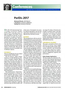
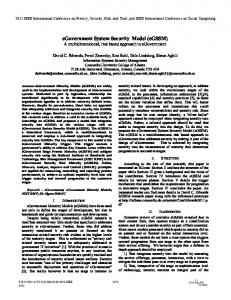
Table 1: Workload generation parameters for the test suites. Phase 1 Mixed
Phase 2 Update heavy
Phase 3 Mixed
Phase 4 Query Heavy
Phase 5 Q:DB3 and U:DB3
U: DB4
U: DB3
Q: DB4
U: DB2
Q: DB3
U:DB1
Q: DB2
Q: DB1
U: DB4
U: DB3
Q: DB4
U: DB2
Q: DB3
U:DB1
Q: DB2
Q: DB1
U: DB4
U: DB3
Q: DB4
U: DB2
Q: DB3
U:DB1
Q: DB2
U: DB4
Q: DB1
U: DB3
Q: DB4
Q: DB3
U:DB1
U: DB2
Q: DB2
Q: DB1
Phase 6 U:DB3 and U:DB4 Phase 7 U:DB4 and Q:DB4 Phase 8 Q:DB4 and Q:DB1
Figure 1: Distribution for the phases in an update workload. Shaded bars denote the focus of the phase. The notation “Q: DB1” denotes queries on database DB1, whereas “U: DB1” denotes updates. The suite comprises four workloads with phase length 50, 100, 200, and 400. An aggressive tuning algorithm is likely to observe good performance across the board, even when transitions are short-lived. A conservative algorithm is likely to view short-lived transitions as noise, and show gains only for larger phase sizes. C2: Queries The second test scenario examines the performance of online tuning as we vary the query complexity of the workload. This parameter affects the level of difficulty for performing automatic tuning. A workload consists of m phases, with the same distribution as in the previous suite. Thus, we have a gradually shifting workload with overlapping phases. The phase length is set to 300 queries, under the assumption that this is long enough for a reasonable algorithm to adapt to each phase. We generate three workloads consisting of simple, moderate, and complex queries respectively. The simple workload is expected to yield the highest gain for any tuning algorithm. The moderate workload exercises the ability of the algorithm to handle multi-column indexes and index interactions. Finally, the complex workload introduces join indexes to the mix. C3: Updates The third suite examines the performance of a tuning algorithm for workloads of queries and updates. A good tuning algorithm must take into account both the benefit and the maintenance overhead of indexes. A workload in this suite consists of 2m phases, following the ordering shown in Figure 1. Each phase applies again an 80-20 rule for the distribution. The ordering of phases creates the following types of phases: mixed, where the same database is both queried and updated; query-heavy, where most of the statements are queries over two different databases; and, update-heavy, where most of the statements are updates over two different databases. The idea is to alternate between phases with a different effect on online tuning. For instance, a queryheavy phase is likely to benefit from the materialization of indexes, whereas an update-heavy phase is likely to incur a high maintenance cost if any indexes are materialized. 5
We generate two workloads with simple and complex updates respectively. In both cases, the queries are of moderate complexity. Clearly, simple updates involve less complicated index interactions and hence the bookkeeping is expected to be simpler. Conversely, we expect online tuning to be more difficult for updates of moderate complexity. C4: Convergence This suite examines online tuning with a stable workload that does not contain any shifts, i.e., the whole workload consists of a single phase. The expectation is that any online tuning algorithm will converge to a configuration that will remain unchanged by the end of the workload. Thus, it is interesting to identify the point in the workload where the configuration “freezes”. The suite consists of a single workload with a single phase of 500 moderate queries and a uniform distribution. This creates a setting where the choice of optimal indexes is less obvious, compared to a phase that focuses on a specific set of databases. C5: Variability The last suite examines the performance of online tuning as we expand the set of attributes that carry selection predicates. The workloads in this suite are identical to suite C2, except that we vary the maximum size of the predicated attribute-sets as 1,2,3, and 4. We expect to observe a direct correlation between the variability of the workload and the effectiveness of an online tuning algorithm, but it is also interesting to observe the relative difference in performance for the different values of the varied parameter.
4
Experimental Study
We performed an experimental study of several online tuning algorithms using the described benchmark. We first describe the setup of the experimental study and the discuss briefly the key results.
4.1
Experimental Setup
Index-Tuning Algorithms. We tested three index tuning algorithms: C OLT[3], BC[1] and WFIT[11]. We chose these algorithms as they have very different features: C OLT employs stochastic optimization to make its tuning decisions; BC employs retrospection over the past workload to choose index-sets, and requires specific machinery from the underlying system; WFIT also employs retrospection, but it relies on standard system interfaces and also carries theoretical performance guarantees on its choices. The three algorithms also have different overheads, with C OLT being the most light-weight and WFIT being the most expensive. We implemented these algorithms with PostgreSQL as the underlying DBMS. We chose PostgreSQL since it is a mature, robust system and the source code is freely available. The implementation required us to extend PostgreSQL with several query- and index-analysis primitives, including a what-if optimizer to estimate the benefit of hypothetical indexes. We also added support for true covering indexes, which can bring significant benefits to query evaluation. DBMS Setup. PostgreSQL reported a total size of 4GB after loading all data and building indexes for primary keys. Of this, 2.9GB was attributed to the base table storage. As specified by the benchmark, we set the index storage budget to the mean of the four database sizes, which in our case was about 750MB. To create an interesting execution environment, we artificially limited the available RAM to 1GB and set the DBMS buffer pool to 64MB.3 We note that we kept a small data scale to ensure timely completion of the experiments.
4.2
Summary of Results
Due to space constraints, we provide only a summary of our findings based on the experimental results. The complete details can be found in the relevant full publications[5, 4]. 3
We followed the practice advocated by PostgreSQL administrators to delegate cache management to the file system.
6
C1: Reflex. All algorithms had improved performance as the phase length increased. Overall, the two retrospective algorithms BC and WFIT performed better than C OLT, which relies on stochastic optimization. One possible explanation is that C OLT had limited data (especially for short phases) on which to make reliable predictions, whereas BC and WFIT employ a retrospective analysis of the complete past workload and avoid predictions altogether. C2: Queries. All algorithms followed the same trend of decreasing performance as the query complexity increased. The retrospective algorithms again performed better than C OLT, although the difference was not drastic for the simplest class of queries. WFIT exhibited a consistent advantage over BC, but the difference was small in all experiments. C3: Updates. The inclusion of updates in the workload resulted in an interesting reversal of the ranking of the three algorithms. WFIT continued to be the top performer, but now C OLT performed better than BC, which took a significant performance hit. One possible explanation is that BC relies on heuristics in order to update benefit statistics with the effects of update statements and index interactions, and these heuristics do not work well for the given workload and the specific DBMS that we employ (the original algorithm was developed for MS SQL Server). C4: Convergence. All algorithms improve the workload, with WFIT offering about twice as much benefit as the other algorithms. As noted in the previous section, the purpose of this experiment is to verify that the algorithms converge quickly, since we expect the online algorithm to be stable when the workload is stable. WFIT excels in this regard: in the second half of the workload, the index materializations of WFIT had a total cost that was two orders of magnitude lower compared to the corresponding costs of C OLT and BC respectively. C5: Variability. As expected, all three algorithms performed best when the maximum size was set to one, which in turn resulted in very few candidate indexes that had a clear benefit. WFIT was the top performer in all cases, followed by BC and C OLT, in that order. BC exhibited an interesting drop in its performance when the set size increased from two to three, which we can attribute to the increase in the intensity of index interactions and the heuristics that BC uses to deal with these interactions. Overhead. There is a noticeable difference between the three algorithms in terms of their overhead, which we separate in two disjoint components: the overhead to analyze each statement in the incoming workload and update internal statistics, and the number of what-if optimizations performed by the algorithm. The reason behind this separation is that the speed of what-if optimization is tightly coupled with the specific DBMS, whereas the first component is specific to the algorithm and hence likely to be unaffected by changes to the DBMS. C OLT has the least analysis overhead of all algorithms, as it is designed to offer a light-weight solution for online index tuning. In fact, C OLT averages less than one what-if call per query, which means that some queries are analyzed without even contacting the what-if optimizer. BC has a higher analysis overhead due to its more complex internal logic, but it does not require any what-if optimization calls. Instead, all analysis is done by examining the optimal plan for executing the query under analysis. WFIT has the highest analysis overhead, with an order of magnitude difference from the other two algorithms. This is due to two factors: WFIT employs a sophisticated analysis of the workload, which enables it to choose indexes with strong performance guarantees; and, the algorithm is implemented in unoptimized Java code that runs on top of the DBMS, whereas both C OLT and BC are implemented in optimized C code inside PostgreSQL. Accordingly, it also performs far more what-if calls than the other two algorithms. Hence, WFIT is a viable choice only if the what-if optimizer is fast, or if it is possible to employ a fast what-if optimization technique such as INUM or CPQO.
5 Lessons Learned The implementation of our benchmark allowed us to gain useful insights on the relative performance, strengths and weaknesses of three online index-tuning algorithms. We strongly believe that the proposed benchmark provides a principled methodology to stress-test online tuning algorithms under several scenarios.
7
At the same time, our experience from implementing the benchmark (and using it subsequently for several experimental studies) has revealed several ways to improve the overall methodology. More concretely, it is important to couple the complex workload suites with simpler micro-benchmark workloads which contain a handful of queries and can thus offer greater visibility in the behavior of an online tuning algorithm. Furthermore, we have observed that the generated workloads have a varying degree of difficulty across different systems. It would be desirable to have a benchmark with a more homogeneous behavior across different DBMSs. In a different direction, we attempted to implement the benchmark in a database-as-a-service environment, in order to gauge the plausibility of online index tuning “in the cloud”. Unfortunately, we were not able to get reliable results due to the extremely high variance of our measurements. Our observations corroborate the results of a more general study by Schad et al.[12] We theorize that the source of this variance was the execution of the DBMS inside a virtual machine at the service provider, and the performance characteristics of distributed block storage vs. local storage. Our take-away message, for now, is that it may be difficult to execute an online tuning algorithm in this environment, given that the what-if optimizer will not be able to accurately predict the actual benefit of different indexes.
References [1] N. Bruno and S. Chaudhuri, “An online approach to physical design tuning,” in ICDE ’07: Proceedings of the 23rd International Conference on Data Engineering, 2007. [2] K.-U. Sattler, M. L¨uhring, I. Geist, and E. Schallehn, “Autonomous management of soft indexes,” in SMDB ’07: Proceedings of the 2nd International Workshop on Self-Managing Database Systems, 2007. [3] K. Schnaitter, S. Abiteboul, T. Milo, and N. Polyzotis, “On-line index selection for shifting workloads,” in SMDB ’07: Proceedings of the 2nd International Workshop on Self-Managing Database Systems, 2007. [4] K. Schnaitter and N. Polyzotis, “A benchmark for online index selection,” in SMDB ’09: Proceedings of the 4th International Workshop on Self-Managing Database Systems. IEEE, 2009, pp. 1701–1708. [5] K. Schnaitter, “On-line index selection for physical database tuning,” Ph.D. dissertation, University of California Santa Cruz, 2010. [6] A. Borodin, N. Linial, and M. E. Saks, “An optimal on-line algorithm for metrical task system,” Journal of the ACM, vol. 39, no. 4, pp. 745–763, 1992. [7] W. R. Burley and S. Irani, “On algorithm design for metrical task systems,” Algorithmica, vol. 18, no. 4, pp. 461–485, 1997. [8] S. Finkelstein, M. Schkolnick, and P. Tiberio, “Physical database design for relational databases,” ACM Trans. Database Syst., vol. 13, no. 1, pp. 91–128, 1988. [9] S. Chaudhuri and V. Narasayya, “Autoadmin “what-if” index analysis utility,” SIGMOD Rec., vol. 27, no. 2, pp. 367–378, 1998. [10] K. Schnaitter, N. Polyzotis, and L. Getoor, “Index interactions in physical design tuning: modeling, analysis, and applications,” Proc. VLDB Endow., vol. 2, 2009. [11] K. Schnaitter and N. Polyzotis, “Semi-Automatic Index Tuning: Keeping DBAs in the Loop,” CoRR, vol. abs/1004.1249, 2010. [12] J. Schad, J. Dittrich, and J.-A. Quian´e-Ruiz, “Runtime measurements in the cloud: Observing, analyzing, and reducing variance,” PVLDB, vol. 3, no. 1, pp. 460–471, 2010.
8