Benefits of an Implicit Redundant Genetic Algorithm Method for

Benefits of an Implicit Redundant Genetic Algorithm Method for Structural Damage Detection in Noisy Environments Anne Raich1 and Tamás Liszkai1 1

Texas A&M University, Department of Civil Engineering, College Station, Texas, 77843, USA {araich, tamas}@tamu.edu

Abstract. In this research, the problem of structural damage detection using noisy frequency response function information is addressed. A methodology for damage detection is proposed that uses an unconstrained optimization problem formulation. To solve the optimization problem genetic algorithms (GA) and a local hillclimbing procedure were used. The inherent unstructured nature of damage detection problems is exploited through the application of an implicit redundant representation (IRR) allowing for the number of decision variables to dynamically change during the course of optimization. To evaluate the proposed damage detection method, test runs for a cantilever beam and an unbraced frame structure were performed. Test case results using different measurement noise levels show that the IRR GA has superior performance over the standard GA fixed representation.

1 Introduction The goal of damage detection procedures is to accurately assess the condition of structures and facilitate decision-making related to structural rehabilitation and maintenance, which could significantly increase performance and service-life while reducing cost. Pioneering research in the field of damage detection started in the 1970s, with the realization that mere visual inspection of fatigue prone structures is not sufficient in maintaining the reliability of aircraft structures and steel bridges [1]. Earlier research found that damage changes the dynamic stiffness of structures and, therefore, natural frequency measurements can be used to detect damage using a finite element model of a structure [2]. Frequency response functions (FRF) were used in [3] to determine the natural frequencies of a longitudinally vibrating beam modeled as two undamaged elements connected by a short one representing the damage. Another approach minimized the Bayesian inference function using a modified Newton-Raphson algorithm to better correlate between the measured and analytical natural frequencies and mode shapes [4]. A comprehensive literature review of existing model parameter updating methods is given in [5], which details the use of FRF data in parameter updating. Although in the last decade research focusing on procedures using modal information has received significant attention [6], in this research we focus on FRF based

procedures. The advantages of using FRF data over modal parameters are that FRF data can be measured directly on structures without any intermediate steps and that FRF data provides information over a frequency range instead of only at certain frequencies. Several researchers have used FRF information for damage detection. Applications using FRF data include iterative procedures [7-8], flexibility method [9], transmittance function matrix information [10], and optimization procedures [11-13]. In recent years, artificial intelligence and machine learning techniques for damage detection have been proposed. Genetic algorithms (GA) have been applied to a variety of damage detection problems, including crack detection in composite materials [14]. A common feature of all genetic algorithm based damage detection techniques is that they employ an error function between the measured data and the discrete analytical model [15-16]. In the research presented, the damage detection problem is formulated as an optimization problem, which is solved using both a simple genetic algorithm (SGA) [17] and an IRR GA to take advantage of the unstructured nature of damage detection. The implicit redundant representation (IRR) of genes [18], which allows the dynamic change or evolution of optimization variables, was applied in [19]. In their approach, however, the authors utilized static equilibrium equations instead of vibration data to set up the optimization problem. In addition neural networks [20] have been successfully applied for damage detection in several studies [21-22], while other researchers attempted to use fuzzy logic with remarkable results even at high noise levels [23].

2 Theory of Damage Detection The underlying principle of most damage detection techniques is that vibration signatures, e.g. FRFs or modal data, are sensitive indicators of structural integrity. Most of the damage detection procedures work with a discrete analytical model of the structure, which can be a finite element model, shear building model, etc. Model parameter updating techniques try to adjust the physical parameters of these models, (such as stiffness, mass and damping properties), using an iterative process. The presented damage detection technique assumes that a finite element model of the undamaged structure is available. 2.1 Finite Element Formulation and FRF Matrices The equations of dynamic analysis of an n-degree of freedom (DOF) viscously damped system can be derived from the principle of virtual work [24]. If the system is excited by a set of sinusoidal forces with ω circular frequency, but with different amplitudes and phases, then the equations of motion are written [25].  + Cu + Ku = f0 e − iω t Mu

(1)

where M, C and K are the mass, damping, and stiffness matrices of the undamaged structure, u is the displacement vector, ω is the circular natural frequency of excitation, f0 is the vector of complex forcing amplitudes, i is the imaginary unit, and t is

time. It is assumed that the solution of the above set of differential equations exists in − iω t

the form u = ze , where z is the vector of time independent complex amplitudes. The formal solution of Equation 1 is obtained in the form. z = (K - iω C - ω M) f0 ≡ Rf0 2

-1

(2)

where the receptance matrix R is defined as a function of ω. The computational expense incurred in obtaining the receptance matrix by means of Equation 2 is prohibitive and therefore not well suited for optimization purposes. To reduce the computational effort involved in the calculation of the receptance matrix it is assumed that the structure is proportionally damped and the principle of superposition holds, i.e. the structure is linear. For a proportionally damped viscous dynamic system, the modal decomposition of the receptance matrix can be written.



 T Φ 2 2   ω j − 2iωζ jω j − ω  1

R = Φ diag 

(3)

where ωj is the jth natural frequency of the system, ζj is the jth modal damping ratio, Φ is the mode shape matrix (each column represents a mode shape), and diag() represents a diagonal matrix. The computational expense of the above expression is remarkably smaller than that incurred by using Equation 2. Depending on the type of measurement data (displacement, velocity, acceleration) a FRF matrix other than the receptance matrix may be desired. The relationships between the receptance, mobility, V, and accelerance, A, matrices appear in Equation 4. V (ω ) = −iω R (ω )

(4)

A (ω ) = −iω V (ω ) = −ω 2 R (ω ) In general the jkth member of an FRF matrix represents the response (displacement, velocity or acceleration) of the jth DOF when the excitation is applied at the kth DOF. 2.2 Damage Indicators When damage affects the properties of structures, such as stiffness, damping and mass, then vibration signatures can be used for damage detection. In general, damage may affect any of the above-mentioned properties. In most cases, however, changes in stiffness properties are the most significant indicators of damage. To reduce the complexity of the damage detection procedure it is assumed that only the stiffness properties are altered by damage. This research assumes that stiffness is altered by changes in the Young’s modulus of the material. To model damage(s) in structures, a damage indicator, x sj , was assigned to each finite element, j, in the model. dam

kj

(

)

= 1− xj k j , 0 ≤ xj ≤ 1 s

s

(5)

dam

where k j

is the stiffness matrix of the jth damaged finite element, kj is the stiff-

ness matrix of the jth finite element without damage, and x j is the damage indicator s

of the jth finite element. The positive damage indicators may be interpreted as percentile damage values from zero to 100 percent. Since all finite elements in the model have a unique damage indicator, the location and severity of damage is also unique. Using the damage indicator vector, any of the FRF matrices of the structure can be obtained for a particular damage case. The goal of the damage detection process is to obtain the vector of damage indicators, xs, for all finite elements in the structure. 2.3 Use of FRF Vibration Signatures in Damage Detection Assuming that FRF data can capture the location and severity of damage, the idea behind the presented damage detection procedure is to minimize some error term between the measured FRF data and the analytical FRF functions computed by means of the damage indicator vector. In this case, the solution of the minimization problem will result in identifying a damage indicator vector that correctly identifies the location and severity of damage(s) in the structure. From the definition of FRF matrices it is obvious that the dimensionality of such matrices may become very large as the number of DOFs in a finite element model increases. As a result, only certain entries of an FRF matrix can be measured in practice. In this research it is assumed that there is only one excitation location, but measurements may be taken simultaneously at multiple locations. The error function between the measured and analytical FRF data is defined in the following expression.

 ϖ1  f = ∑  ∫ Ajk (ω ) − Ajk (ω ) dω  k ∈J  ϖ  nmeas

2

(6)

0

where j is the excitation DOF, k is the DOF where the response is measured, Ajk is the jkth analytical accelerance FRF in the finite element model, Ajk is jkth measured accelerance FRF, J is the set of measurement DOFs, nmeas is the number of measurement DOFs, ϖ0 and ϖ1 are the lower and upper frequencies of the measured frequency range, and the symbol indicates complex magnitude. This objective function poses an unconstrained optimization problem in which the unknown variables are the damage indicators.

3 Optimization Algorithm In recent decades with the development of computer technology, a new generation of optimization algorithms targeting a wide range of optimization problems were developed. GAs provide an approach to optimization that mimic nature’s evolutionary mechanism and Darwin’s “survival of the fittest” theory. The foundations of genetic

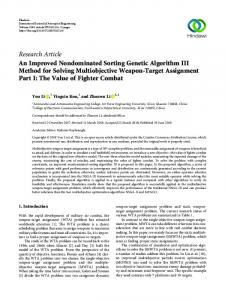
algorithms supported by the schema theorem and minimal building blocks can be found in [23, 26]. In the simple genetic algorithm (SGA), genes are typically represented in a fixed binary format and the common operations such as selection, crossover and mutation are applied to evolve the next generation of individuals. 3.1 Unstructured Optimization Domain in Damage Detection The fixed gene representation for damage detection used by the SGA encodes as design variables a damage indicator that uniquely identifies the location and severity of damage for each finite element in the model (Fig. 1a). The gene length using the fixed SGA representation is allocated in accordance with the number of finite elements in the model and the number of binary digits required for a certain precision of the damage indicators. One of the shortcomings of the fixed SGA representation is that each string is a genotype representation of the whole problem domain and therefore can become very large. For the damage detection problem, however, even when the number of finite elements in the model becomes very large the number of damaged elements is only a fraction of the number of finite elements in the model. This special situation defines an optimization problem in which the number of independent variables is unknown and is somewhere between zero and the number of finite elements in the model. The implicit redundant representation [18] can overcome the difficulties associated with the unstructured damage detection problem identified. The implicit redundant representation (IRR) introduces redundant segments into the gene string, which allows the number of variables to dynamically change during the course of optimization [18]. This property is appealing for damage detection problems in which neither the number of damaged elements nor their locations are known beforehand. The redundant and useful segments in an IRR string interact dynamically by using a string length that is longer than the length required to encode the parameter values. A typical IRR gene for the damage detection problem is depicted in Fig. 1b. A segment of the encoded IRR string, which currently carries useful information, is called a gene instance. A gene instance consists of the gene locator (GL) pattern, a segment encoding the finite element number (location of damage), and a segment encoding the damage indicator for that finite element (magnitude of damage). Gene instances encode the parameter values using binary bit encodings similar to other GAs. In the IRR GA, however, redundant segments between any two consecutive gene instances may become useful segments in later generations through the actions of genetic operations. The IRR does not require the number of parameter values to be specified since the number of gene instances can change dynamically to reach a better solution implicitly implied in the objective function. The trials presented in this paper were based on a simple GL pattern of [1 1 1] for the binary encoded IRR. To decode the parameter values the gene is parsed until a GL pattern is found identifying the beginning of a gene instance. In the fixed SGA representation each individual in the population represents one complete solution to the problem, which contains a damage indicator for each element in the model. For the IRR GA, each individual in the population also represents one complete solution, but a solution is defined only by the damage indicators for a small subset of the finite elements in the model, instead of all.

... Element 1

Element 3

Redundant segment

Element ne ... Element 2

(a) Fixed Representation

Gene Instance

1 1 1 0 1 1 0 0 0 1 1 1 0 Gene locator Encoded finite element number

Encoded damage indicator

(b) Implicit Redundant Representation IRR

Fig. 1. Differences in fixed SGA representation and implicit redundant representation (IRR) for damage detection

3.2 Implementation and Local Search Capabilities The proposed damage detection procedure was implemented in C++ using the MATLAB C/C++ Math Library [28]. Besides the usual genetic operators characteristic to SGAs [23], advanced operators, which include adaptive and equal probability multi-point crossover, uniform and non-uniform mutation, tournament selection, elitism, binary and Gray coding of variables, and encoding solutions in fixed and IRR representations, are also implemented in the program [27]. Non-uniform mutation is only used for the fixed SGA representation. For the IRR GA, the string length is obtained from the number of significant digits for the damage indicator and the user defined expected number of gene instances in the string [18]. The expected number of gene instances is directly related to the number of possibly damaged elements in the model, which is usually significantly less than the number of finite elements in the model. To overcome the slow convergence rate near the global optimum that is characteristic to GAs, a local hillclimbing search technique is implemented to allow fine-tuning of the results obtained by the GA. In this implementation, the step size for each variable changes independently based on the success or failure of hillclimbing for the specific variable. A reduced version of hillclimbing is also available, in which hillclimbing is only carried out for variables having a damage indicator greater than zero.

4 Test Cases and Measurement Noise Case studies were performed on a cantilever beam (Fig. 2) and a three-story three-bay unbraced frame structure (Fig. 3) to evaluate the sensitivity of the proposed damage detection procedure to noise in the measurements. Trials were performed using both the fixed representation and the IRR representation to compare their performance. In Figs. 2-3 regular numbers indicate node numbers and element numbers are in italics. All finite elements are Bernoulli type frame elements. The cantilever beam is a

W12 × 65 with an area of A = 0.0123 m2 (19.1 in2) and second moment of inertia I = 2.218⋅10-4 m4 (533 in4). The cantilever model is defined by 11 nodes and 10 finite elements. For the unbraced frame problem, all columns (W14 ×132, A = 0.025 m2 (38.8 in2) I = 6.368⋅10-4 m4 (1530 in4)) are modeled using 3 finite elements, and all beams (W12 ×65) are modeled with 5 finite elements. A total of 76 nodes and 81 elements are defined in the frame model. The Young’s modulus of steel is E = 207 GPa (30,000 ksi), Poisson’s ratio is ν = 0.3, and the mass density is ρ = 7780 kg/m3 (0.000728 lb-s2/in4) for all cases. 7.62 m (25 ft) 1

2 1

3 2

4 3

5 4

6 5

7 6

8 7

9 8

10 11 9

10

Fig. 2. Cantilever beam finite element mesh (node numbers are regular and element numbers are in italics)

9.14 m (30 ft)

3.66 m (12 ft) 3.66 m (12 ft)

9.14 m (30 ft)

69 52 36

28

71 61 39

67 42

58

31

22

54

33 12

59 21

4.57 m (15 ft)

7.62 m (25 ft)

6

45 14

16

2

10

18

Fig. 3. Three-story three-bay unbraced frame structure finite element mesh (node numbers are regular and element numbers are in italics)

Simulated measurement FRF data were generated for the two test cases using the defined parameters in Table 1. In both cases, a 10% damage was imposed on a single finite element. For the cantilever problem (CANT), the damaged element is located close to the fixed support (element 2), the excitation is placed at the free end (node 11) and the measurement is taken about the mid-span (node 7). For the frame problem the inflicted damage is found on the first floor exterior beam (element 21), and three measurement locations (nodes 59, 67, 69) and the excitation at the upper story (node 71) are used for generating the simulated FRF data.

Table 1. Parameters defined for cantilever (CANT) and unbraced frame (FRM) test cases

Case CANT FRM

Imposed Damage Element Magnitude 2 10 % 21 10 %

Excitation

Measurement

11 71

7 59, 67, 69

To introduce noise into the measurements, normally distributed random noise was added to the simulated FRF data with zero mean and a variance of 1. The accelerance FRF including noise is obtained from the FRF without noise using the following equation. Ajk = Ajk (1 + yn randn() )

(7)

where Ajk is jkth measured FRF including noise, Ajk is the jkth measured FRF without noise, yn is the noise level (e.g. 0.05 relates to a 5 % noise level) and randn() is the random noise generator function in MATLAB [28].

5 Results and Discussions Initial trials were performed to find a good combination of GA input parameters that were used later in the runs. For the cantilever beam trials, the population size was 100, the mutation rate was 10 %, and the maximum number of generations was 200. Furthermore Gray coding, elitism, and adaptive crossover with a 90 % primary and a 100 % secondary crossover rate were used. The number of individuals competing in tournament selection was 4 and 8, and the number of crossover sites was 8 and 10 for the fixed and for the IRR representations, respectively. For the frame structure trials, the population size was increased to 200 and the maximum number of generation to 300. Otherwise the input parameters were similar to those for the cantilever trials. In certain trials (all trials with fixed representation, cantilever beam trials with IRR GA) the initial population was seeded with a zero damage individual. For the fixed representation a zero damage individual is obtained if all digits in the gene are zero. For the IRR GA, the decoded damage indicator segment of a gene instance is zeroed out. 5.1 Cantilever Beam Test Case To investigate the effect of measurement noise on the accuracy of damage detection five different noise levels (0, 5, 10, 20, 50 %) were used for the cantilever problem. The number of expected gene instances (damaged elements) for the IRR GA was set to five. In Fig. 4 and 5 results for the fixed and IRR gene representations are depicted, respectively. From the figures it is clear that the imposed damage location (element 2) and magnitude (10 %) was identified by both representations for the noise free (0 %) measurement cases. In case of the fixed representation, however, the global optimum was not obtained after 200 generations and it took 1492 hillclimbing iterations to find the exact damage indicators. The IRR GA found the global optimum after 130 genera-

Percent damage

tions and there was no need for additional hillclimbing iterations. In the initial IRR population the best individual had five gene instances, which identified five different elements in the model as damaged. In the best IRR individual in the final population, however, there were only two gene instances defined and both identified the same correct damaged element and the average of the decoded damage indicators was the imposed 10 % value. 12% 10% 8% 6% 4% 2% 0%

0 % Noise 10 % Noise 50 % Noise

1

2

3

4

5

6

5 % Noise 20 % Noise

7

8

9

10

Finite element number

Percent damage

Fig. 4. Damage detection results for the cantilever beam problem using fixed representation after 200 generations without hillclimbing, seeded initial population with zero damage individual

12% 10% 8% 6% 4% 2% 0%

0 % Noise 10 % Noise 50 % Noise

1

2

3

4

5

6

5 % Noise 20 % Noise

7

8

9

10

Finite element number Fig. 5. Damage detection results for the cantilever beam problem using IRR after 200 generations without hillclimbing, initial population is not seeded with zero damage individual

The accuracy of damage detection degrades with increasing noise levels in the measurements regardless of the representation used. The figures show, however, that the IRR GA better approximates the original damage case than the fixed representation at any noise level. Using the fixed representation, the number of elements identified as damaged were 5 to 9 out of the 10 elements while for the IRR GA it was always 3 (except the noise free case when it was 1). The IRR GA always found the damaged element and the severity of damage for the falsely identified elements was small or negligible. At very high 50 % noise level (in practice the anticipated noise level is about 5-10 %) the fixed representation breaks down and identification of the correct damaged element is ambiguous. This is not the case for the IRR GA, which

finds the correct damaged element even at 50 % noise level. In addition improvements of the results obtained using the fixed representation were noticeable after hillclimbing, while these improvements were negligible for the IRR GA. 5.2 Unbraced Frame Test Case

Percent damage

For the unbraced frame problem, four different noise levels were investigated (0, 10, 20, 30 %). The number of expected gene instances (damaged elements) for the IRR GA was set to 15. Results obtained using the IRR GA after 300 generations and hillclimbing are shown in Fig. 6. In the case of the fixed representation, none of the trials obtained the correct location or severity of the imposed damage. Therefore results obtained for the fixed representation are not presented. 12% 10% 8% 6% 4% 2% 0%

0 % Noise 20 % Noise

6

10 % Noise 30 % Noise

12 14 21 22 31 33 36 39 42 45 52 54 58 61 Finite element number

Fig. 6. Damage detection results for the unbraced frame problem after 300 generations and reduced hillclimbing using IRR, seeded initial population with zero damage individual

Without noise in the measurement system, the IRR GA was able to find the global optimum after 241 generations. The correct damaged element was identified at all noise levels with close to the exact 10 % damage value and the correct location at element 21. As the level of noise in the measurements increased the number of falsely identified elements with observable damage magnitude increased. Up to a noise level of 20 % the damaged element was identified with considerably higher damage indicator than those of the falsely identified elements. The error in damage detection became significant at a noise level of 30 % and the identification of the damaged element was at that point ambiguous. For the noise free case, initially the best IRR individual had 15 gene instances, while the best IRR individual in the final population had 3 gene instances - one that identified the correct damaged element and two others that identified an element with zero damage. When noise was present in the measurements, the number of gene instances changed from 15 in the initial population to 810 in the final population. Hillclimbing somewhat improved the solutions obtained by the IRR GA, but not significantly.

6 Conclusions In this paper the effect of measurement noise on the accuracy of damage detection was studied. The proposed damage detection method uses the information inherent in FRF data to identify the location and severity of damage(s) in structures. An error function between the analytical and measured FRF data is defined posing an unconstrained minimization problem, which is solved using genetic algorithms and a local hillclimbing search. Two different types of GA representations were investigated. A fixed representation, in which the number of decision variables equals to the number of finite elements in the model and an IRR representation which considers the unstructured nature of damage detection problems by allowing the number of damaged elements to change during optimization. Case studies show that the IRR GA outperforms the fixed representation SGA in all trials. Use of the fixed representation is limited to problems with a relatively small number of decision variables or damage indicators (no solution was found for the unbraced frame problem). To obtain the results presented, the initial population of fixed representation SGA had to be seeded. The fixed representation SGA also had higher sensitivity on the accuracy of damage detection using noisy FRF data when compared to the IRR GA. Since the fixed representation SGA always operates on all of the damage indicators in the finite element model, the number of falsely identified damaged elements is high even though the severity of damage of the falsely identified elements remains small. In comparison, the adaptive characteristic of the IRR GA was shown to be well suited for damage detection problems, as the number of damage indicators is not explicitly encoded in the IRR GA. The IRR GA can determine the number of damaged elements, while minimizing the error between the measured and analytical FRF information. In a noise free environment the global optimum was always found and the IRR GA was considerably less sensitive to measurement noise compared with the fixed representation. Even for large problems, the IRR GA was capable of identifying the damaged elements due to encoding only a subset of all possible finite elements. Seeding the initial population was not necessary to find the solution, but was advantageous in certain situations.

References 1. Liu, S-C., Yao, J.T.P.: Structural Identification Concept. Journal of the Structural Division, ASCE 104(ST12) (1978) 1845-1858 2. Cawley, P., Adams, R.D.: The location of defects in structures from measurements of natural frequencies. Journal of Strain Analysis 14(2) (1979) 49-57 3. Springer, W.T., Lawrence, K.L., Lawley, T.J.: Damage assessment based on the structural frequency-response function. Experimental Mechanics 28(1) (1988) 34-37 4. Béliveau, J-G., Chater, S.: System identification of structural dynamic parameters from modal data. Computational Methods and Experimental Measurements: Proceedings of the international conference, Washington, D.C., Berlin–New York, Springer-Verlag (1982) 40-50 5. Mottershead, J.E., Friswell, M.I.: Model updating in structural dynamics: A survey. Journal of Sound and Vibration 167(2) (1993) 347-375

6. Kim, J.T., Stubbs, N.: Improved damage detection identification method based on modal information. Journal of Sound and Vibration 252(2) (2002) 223-238 7. Wang, Z., Lin, R.M., Lim, M.K.: Structural damage detection using measured FRF data. Computer Methods in Applied Mechanics and Engineering 147 (1997) 187-197 8. Lee, U., Shin, J.: A frequency response function-based structural damage identification method. Computers & Structures 80 (2002) 117-132 9. Park, K.C., Reich G.W., Alvin, K.F.: Structural damage detection using localized flexibilities. Structural health monitoring: current status and perspectives: proceedings of the International Workshop on Structural Health Monitoring: Stanford University, Stanford, CA, September 18-20 1997, Lancaster, PA: Technomic Pub. (1997) 125-139 10. Schulz, M.J., Naser, A. S., Pai, P. F., Linville, M.S., Chung, J.: Detecting structural damage using transmittance functions. Proceedings of the 15th International Modal Analysis Conference, February 3-6, Orlando, Florida, Bethel, CT: Society for Experimental Mechanics INC. (1997) 638-644 11. Dunn, S.A.: The use of genetic algorithms and stochastic hill-climbing in dynamic finite element model identification. Computers & Structures 66(4) (1998) 489-497 12. Luber, W.: Structural damage localization using optimization method. Proceedings of the 15th International Modal Analysis Conference, February 3-6, Orlando, Florida, Bethel, CT: Society for Experimental Mechanics INC. (1997) 1088-1095 13. Thyagarajan, S.K., Schulz, M.J., Pai, P.F.: Detecting structural damage using frequency response functions. Journal of Sound and Vibration 210(1) (1998) 162-170 14. Xu, Y.G., Liu, G.r., Wu, Z.P.: Damage detection for composite plates using lamb waves and projection genetic algorithm. AIAA Journal 40(9) (2002) 1860-1866 15. Chiang, D-Y., Lai, W-Y.: Structural damage detection using the simulated evolution method. AIAA Journal Technical notes 37(10) (1999) 1331-1333 16. Moslem, K., Nafaspour, R.: Structural damage detection by genetic algorithms. AIAA Journal 40(7) (2002) 1395-1401 17. Goldberg, D.E.: Genetic algorithm in search, optimization, and machine learning. Reading Mass. Addison-Wesley Pub. Co. (1989) 18. Raich, A.M., Ghaboussi, J.: Implicit redundant representation in genetic algorithms. Evolutionary Computation 5(3) (1997) 277-302 19. Chou, J-H., Ghaboussi, J.: (2001). “Genetic algorithm in structural damage detection. Computers and Structures 79 (2001) 1335-1353 20. Haykin, S.S.: Neural networks: A comprehensive foundation. Upper Saddle River N.J. Prentice Hall (1999) 21. Yun, C-B., Bahng, E.Y.: Substructural identification using neural networks. Computers and Structures 77 (2000) 41-52 22. Marwala, T.: Damage identification using committee of neural networks. Journal of Engineering Meachanics 126(1) (2000) 43-50 23. Sawyer, J.P., Rao, S.S.: Structural damage detection and identification using fuzzy logic. AIAA Journal 38(12) (2000) 2328-2335 24. Cook, R.D., Malkus, D.S., Plesha, M.E., Witt, R.J.: Concepts and applications of finite element analysis. New York Wiley (2002) 25. Gatti, P., Ferrari, V.: Applied structural and mechanical vibrations. London – New York E & FN Spon (1999) 26. Holland, J.H.: Adaptation in natural and artificial systems. Ann Arbor, MI: The University of Michigan Press. (1975) 27. Michalewicz, Z.: Genetic algorithms + data structures = evolution programs. Berlin – New York: Springer-Verlag (1996) 28. MATLAB C/C++ math library 2.1 user’s guide. Natick, MA: The Mathworks Inc. (1999)