Beta regression modeling: recent advances in theory and applications ... Simple
beta regression models are similar to generalized linear models. Some early ......
Alternative estimating and testing empirical strategies for fractional regression ...
Beta regression modeling: recent advances in theory and applications Silvia L. P. Ferrari
February, 2013
˜ - Maresias - SP 13a Escola de Modelos de Regressao
1 / 45
Silvia L. P. Ferrari
Beta regression modeling: recent advances in theory and applications
Introduction
Data measured in a continuous scale and restricted to the unit interval, i.e. 0 < y < 1:
2 / 45
I
percentages,
I
proportions,
I
fractions,
I
rates.
Silvia L. P. Ferrari
Beta regression modeling: recent advances in theory and applications
Introduction Examples I
percentage of time devoted to an activity;
I
fraction of income spent on food;
I
unemployment rate, poverty rate, etc.;
I
math score, reading score, etc.;
I
Gini’s index;
I
fraction of “good cholesterol” (HDL/total cholesterol);
I
proportion of sand in the soil; fraction of surface covered by vegetation.
I
More later...
3 / 45
Silvia L. P. Ferrari
Beta regression modeling: recent advances in theory and applications
Introduction Limited range variables usually display: I
heteroskedasticity (the variance is smaller near the extremes);
I
asymmetry.
A possible solution for regression analysis is to employ a transformation in the response, and use normality assumption. For example, ye = log[y /(1 − y)]. Drawbacks:
4 / 45
I
difficult to correct for both heteroskedasticity and asymmetry;
I
the model parameters cannot be easily interpreted in terms of the original response.
Silvia L. P. Ferrari
Beta regression modeling: recent advances in theory and applications
Introduction It is more appropriate to use a regression model that assumes that the response variable follows a continuous distribution with support in (0, 1). Example: Beta regression.
Beta regression models employ a parameterization of the beta distribution in terms of its mean and a precision (or dispersion) parameter.
Simple beta regression models are similar to generalized linear models.
Some early references: Paolino (2001); Kieschnick & McCullough (2003); Ferrari & Cribari–Neto (2004); Cepeda & Gamerman (2005). 5 / 45
Silvia L. P. Ferrari
Beta regression modeling: recent advances in theory and applications
Beta regression models Beta density: f (y ; µ, φ) =
Γ(φ) y µφ−1 (1 − y )(1−µ)φ−1 , 0 < y < 1, Γ(µφ)Γ((1 − µ)φ)
where 0 < µ < 1 and φ > 0. Note that E(y ) = µ and var(y ) =
µ(1 − µ) . 1+φ
Hence, φ can be regarded as a precision parameter. This is not the usual parameterization of the beta law, but is convenient for modeling purposes.
6 / 45
Silvia L. P. Ferrari
Beta regression modeling: recent advances in theory and applications
(0.05,5)
(0.95,5) (0.05,15)
(0.95,15)
10
density
6
(0.10,15)
5
4
density
8
10
15
12
Beta regression models
(0.25,15) (0.25,5)
(0.75,5)
(0.90,15) (0.50,15)
(0.75,15)
0
0
2
(0.50,5)
0.0
0.2
0.4
0.6
0.8
1.0
0.0
0.2
0.4
0.6
0.8
1.0
y
(0.05,50)
20
15
y
(0.95,50)
(0.95,100)
(0.90,50)
(0.25,50)
(0.75,50)
10
density
(0.10,50)
(0.10,100)
density
10
15
(0.05,100)
(0.90,100)
(0.25,100)
(0.75,100) (0.50,100)
0
0
5
5
(0.50,50)
0.0
0.2
0.4
0.6
0.8
1.0
y
0.0
0.2
0.4
0.6
0.8
1.0
y
Figure 1. Beta densities for different combinations of (µ, φ). 7 / 45
Silvia L. P. Ferrari
Beta regression modeling: recent advances in theory and applications
A simple beta regression model
Ref.: Ferrari & Cribari–Neto (2004) I
y1 , . . . , yn : independent r.v.;
I
yt , t = 1, . . . , n, follow a beta distribution with mean µt and unknown precision φ, i.e. yt ∼ Beta(µt , φ);
I
g(·): strictly monotone and twice differentiable link function that maps (0, 1) to R. Pk g(µt ) = i=1 xti βi = ηt ;
I
8 / 45
I
β = (β1 , . . . , βk )> ∈ R is a vector of unknown regression parameters;
I
xt1 , . . . , xtk are observations on k covariates (k < n).
Silvia L. P. Ferrari
Beta regression modeling: recent advances in theory and applications
A simple beta regression model Some possible link functions: 1. Logit: g(µ) = log[µ/(1 − µ)]; 2. Probit: g(µ) = Φ−1 (µ); 3. Complimentary log–log: g(µ) = log[− log(1 − µ)]; 4. Log-log: g(µ) = − log[− log(µ)]; 5. Cauchit: g(µ) = tan[π(µ − 0.5)].
9 / 45
I
The link functions above are the inverse cumulative distribution functions (quantile functions) of well-known distributions (1. logistic, 2. standard normal, 3. minimum extreme value, 4. maximum extreme value, 5. Cauchy).
I
For a discussion on link functions, see Ramalho, Ramalho & Murteira (2010).
Silvia L. P. Ferrari
Beta regression modeling: recent advances in theory and applications
A simple beta regression model Log-likelihood: `(β, φ) =
n X
`t (µt , φ),
t=1
where `t (µt , φ)
= log Γ(φ) − log Γ(µt φ) − log Γ((1 − µt )φ) +(µt φ − 1) log yt + {(1 − µt )φ − 1} log(1 − yt ).
Let yt∗ = log
yt 1 − yt
and µ∗t = E(yt∗ ) = ψ(µt φ) − ψ((1 − µt )φ).
10 / 45
Silvia L. P. Ferrari
Beta regression modeling: recent advances in theory and applications
A simple beta regression model Score function for β: Uβ (β, φ) = φX> T (y ∗ − µ∗ ), where X is an n × k matrix whose t-th row is x> t , T = diag{1/g 0 (µ1 ) . . . , 1/g 0 (µn )}, y ∗ = (y1∗ , . . . , yn∗ )> and µ∗ = (µ∗1 , . . . , µ∗n )> .
Score function for φ: Uφ (β, φ)
=
n X
{µt (yt∗ − µ∗t ) + log(1 − yt )
t=1
− ψ((1 − µt )φ) + ψ(φ)}.
11 / 45
Silvia L. P. Ferrari
Beta regression modeling: recent advances in theory and applications
A simple beta regression model Fisher information: � K = K (β, φ) =
Kββ Kφβ
� Kβφ , Kφφ
> where Kββ = φX> WX , Kβφ = Kφβ = X> Tc, Kφφ = tr(D), W = diag{w1 , . . . , wn }, c = (c1 , . . . , cn )> and D = diag{d1 , . . . , dn }, with 1 wt = φ {ψ 0 (µt φ) + ψ 0 ((1 − µt )φ)} 0 , {g (µt )}2
ct = φ {ψ 0 (µt φ)µt − ψ 0 ((1 − µt )φ)(1 − µt )} , dt = ψ 0 (µt φ)µ2t + ψ 0 ((1 − µt )φ)(1 − µt )2 − ψ 0 (φ).
β and φ are not orthogonal.
12 / 45
Silvia L. P. Ferrari
Beta regression modeling: recent advances in theory and applications
A simple beta regression model In large samples, ! �� � � βb β −1 ∼ Nk+1 ,K , φ φb approximately, where βˆ and φˆ are the MLEs of β and φ, and � � ββ K K βφ −1 −1 , K = K (β, φ) = K φβ K φφ where K
ββ
� � 1 > X> Tcc> T> X (X> WX )−1 −1 = (X WX ) Ik + , φ γφ
with γ = tr(D) − φ−1 c> T> X (X> WX )−1 X> Tc, K βφ = (K φβ )> = −
13 / 45
1 > (X WX )−1 X> Tc, K φφ = γ −1 . γφ
Silvia L. P. Ferrari
Beta regression modeling: recent advances in theory and applications
A simple beta regression model
14 / 45
I
MLEs: obtained numerically by maximizing the log-likelihood function.
I
Ferrari & Cribari–Neto (2004) suggest reasonable initial estimates for β and φ.
I
Also in Ferrari & Cribari–Neto (2004): some simple diagnostic tools and applications.
I
R implementation of beta regression inference and diagnostics: betareg package (Cribari–Neto & Zeiles, 2010).
I
A Bayesian approach to beta regression: Branscum, Johnson & Thurmond (2007).
Silvia L. P. Ferrari
Beta regression modeling: recent advances in theory and applications
More general beta regression models
15 / 45
I
Varying dispersion beta regression models: the mean and the precision parameters are modeled through linear regression structures. Smithson & Verkuilen (2006).
I
A general class of beta regression models: the mean and the precision parameters are modeled through linear or nonlinear regression structures. Simas, Barreto-Souza & Rocha (2010).
I
Inflated beta regression models: allow zero and/or one occurrences by incorporating degenerate distributions to model the extreme values. Cook, Kieschnick, McCullough (2008), Ospina & Ferrari (2010, 2012a), Calabrese (2012).
I
Truncated inflated beta regression models: allow truncation in a subset [c, 1] of the unit interval, and mass points at c, zero and one. Pereira, Botter & Sandoval (2011, 2013).
Silvia L. P. Ferrari
Beta regression modeling: recent advances in theory and applications
More general beta regression models I
Semi-parametric beta regression: Branscum, Jonhson & Thurmond (2007), Weihua et al (2012).
I
Time series: Rydlewski (2007), Rocha & Cribari–Neto (2009), Billio & Casarin (2011), Casarin, Dalla Valle, Leisen (2012); da-Silva, Migon & Correia (2011), da-Silva & Migon (2012), Guolo & Varin (2012). Multivariate beta regression: Souza & Moura (2012a, 2012b)
I I
Mixed beta regression: Zimprich (2010), Verkuilen & ˜ Smithson (2012), Figueroa–Zu´ niga, Arellano–Valle & Ferrari (2013), Bonat, Ribeiro Jr & Zeviani (2013).
I
Errors-in-variables beta regression models: Carrasco, Ferrari, Arellano–Valle (2012) (more later). ´ & Beta rectangular regression models: Bayes, Bazan Garc´ıa (2012).
I
16 / 45
Silvia L. P. Ferrari
Beta regression modeling: recent advances in theory and applications
Special topics in beta regression I
Diagnostics: I
I
I
17 / 45
Espinheira, Ferrari, Cribari–Neto (2008a, 2008b) and Chien (2011, 2012) [beta regression with constant precision] Ferrari, Espinheira & Cribari–Neto (2011), Rocha & Simas (2011) [varying dispersion/nonlinear beta regression models] Anholeto, Sandoval & Botter (2012) [beta regression with constant precision; adjusted residuals]
I
Specification tests: Ramalho, Ramalho & Murteira (2010) [with review on models for fractional data], Pereira & Cribari–Neto (2013).
I
Robust inference in varying dispersion beta regression: Cribari–Neto & Souza (2012).
I
Optimal designs: Wu, Fedorov & Propert (2005).
Silvia L. P. Ferrari
Beta regression modeling: recent advances in theory and applications
Special topics in beta regression I
Consistency and asymptotic normality of MLEs: Rydlewski & Mielczarek (2012).
I
Bias correction of MLEs: I
I I
I
Size-corrected tests: I
I
I
I
18 / 45
Ospina, Cribari–Neto, Vasconcellos (2006) and Kosmidis & Firth (2010) [beta regression with constant precision] Simas, Barreto-Souza & Rocha (2010) [general beta regression] Ospina & Ferrari (2012b) [inflated beta regression] Ferrari & Pinheiro (2011) [general beta regression; Skovgaard’s adjustment] Bayer & Cribari–Neto (2012) [simple beta regression; Bartlett correction] Cribari–Neto & Queiroz (2012) [varying dispersion beta regression; Skovgaard, bootstrap, comparison among various tests] Pereira & Cribari–Neto (2012) [inflated beta regression; Skovgaard]
Silvia L. P. Ferrari
Beta regression modeling: recent advances in theory and applications
Errors-in-variables beta regression Ref.: Carrasco, Ferrari, Arellano–Valle (2012) I
yt ∼ Beta(µt , φt ), for t = 1, . . . , n;
I
mean and precision submodels: g(µt ) h(φt )
19 / 45
> = z> t α + xt β,
=
v> t γ
+
m> t λ;
(1) (2)
I
α ∈ Rpα , β ∈ Rpβ , γ ∈ Rpγ , λ ∈ Rpλ are column vectors of unknown parameters;
I
xt = (xt1 , · · · , xtpβ )> and mt = (mt1 , · · · , mtpλ )> are unobservable (observed with error) covariates;
I
the vectors of covariates measured without error, zt and vt , may contain variables in common, and likewise, xt and mt .
I
given the covariates, y1 , . . . , yn are assumed to be independent.
Silvia L. P. Ferrari
Beta regression modeling: recent advances in theory and applications
Errors-in-variables beta regression I I I
st : vector containing all the unobservable covariates; wt is observed in place of st ; it is assumed that wt = τ 0 + τ 1 ◦ st + et ,
I
I I
I I
I
I 20 / 45
(3)
where et is a vector of random errors, τ 0 and τ 1 are (possibly unknown) parameter vectors and ◦ is the element-wise product; τ 0 and τ 1 : additive and multiplicative biases of the measurement error mechanism, respectively; classical additive model: wt = st + et ; we follow the structural approach; the unobservable covariates are regarded as random variables; we assume that s1 , . . . , sn are iid; it is assumed that they are independent of the measurement errors e1 , . . . , en ; the normality assumption for the joint distribution of st and et is assumed; parameters of the joint distribution of wt and st : δ. Silvia L. P. Ferrari
Beta regression modeling: recent advances in theory and applications
Errors-in-variables beta regression I
(y1 , w1 ), . . . , (yn , wn ): observable variables.
I
We omit the observable vectors zt and vt in the notation as they are non-random and known.
I
The joint density of (yt , wt ) is obtained by integrating the joint density of the complete data (yt , wt , st ), f (yt , wt , st ; θ, δ) = f (yt |wt , st ; θ)f (st , wt ; δ), with respect to st .
I
I
21 / 45
θ = (α> , β > , γ > , λ> )> represents the parameter of interest, and δ is the nuisance parameter. The joint density associated to the measurement error model, f (wt , st ; δ), can be written as f (wt , st ; δ) = f (wt |st ; δ)f (st |δ) as well as f (wt , st ; δ) = f (st |wt ; δ)f (wt |δ).
Silvia L. P. Ferrari
Beta regression modeling: recent advances in theory and applications
Errors-in-variables beta regression I
I
We assume that, given the true (unobservable) covariates st , the response variable yt does not depend on the surrogate covariates wt ; i.e. f (yt |wt , st ; θ) = f (yt |st ; θ). The density function of (yt , wt ) is given by Z ∞ Z ∞ f (yt , wt ; θ, δ) = ... f (yt , wt , st ; θ, δ)dst , −∞ −∞ Z ∞ Z ∞ = ... f (yt |st ; θ)f (wt , st ; δ)dst . −∞
I
Log-likelihood function: `(θ, δ) =
n X t=1
=
n X t=1
I I 22 / 45
−∞
Z
∞
∞
Z ···
log −∞
f (yt |st ; θ)f (st |wt ; δ)f (wt ; δ)dst , −∞
log f (wt ; δ) +
n X
Z
∞
i=1
Z
∞
···
log −∞
f (yt |st ; θ)f (st |wt ; δ)dst . −∞
The likelihood function involves analytically intractable integrals. Approximate inference methods needed. Silvia L. P. Ferrari
Beta regression modeling: recent advances in theory and applications
Errors-in-variables beta regression
In order to facilitate the description of the estimation methods, we consider the following model: yt |xt , xt ∼ Beta(µt , φt ), g(µt ) = z> t α + xt β, ind
h(φt ) = v> t γ + xt λ, ind
wt = τ0 + τ1 xt + et , xt ∼ N(µx , σx2 ), et ∼ N(0, σe2 ), with xt and et 0 , for t, t 0 = 1, . . . , n, being independent. The unknown parameter vectors α and γ were defined above, and β ∈ R, λ ∈ R, µx ∈ R and σx2 > 0 are unknown parameters.
23 / 45
Silvia L. P. Ferrari
Beta regression modeling: recent advances in theory and applications
Errors-in-variables beta regression We have ind
ind
wt ∼ N(τ0 + τ1 µx , τ12 σx2 + σe2 ), xt |wt ∼ N(µxt |wt , σx2t |wt ), where µxt |wt = µx + kx [wt − (τ0 + τ1 µx )], σx2t |wt = σe2 kx /τ1 , with kx = τ1 σx2 /(τ12 σx2 + σe2 ) being known as the reliability ratio. To avoid non-identifiability of parameters we assume that (τ0 , τ1 , σe2 ) or (τ0 , τ1 , kx ) are either known parameters or they are estimated from supplementary information, typically replicate measurements or partial observation of the error-free covariate. In any case, either of these vectors are regarded as known quantities in the inferential procedure. Hence, the nuisance parameter vector is δ = (µx , σx2 )> . 24 / 45
Silvia L. P. Ferrari
Beta regression modeling: recent advances in theory and applications
Errors-in-variables beta regression Log-likelihood function: `(θ, δ) =
n X
`1t (δ) +
t=1
n X
`2t (θ, δ),
t=1
where 1 [wt − (τ0 + τ1 µx )]2 `1t (δ) = − log[2π(τ12 σx2 + σe2 )] − , 2 2(τ12 σx2 + σe2 ) " # Z ∞ (xt − µxt |wt )2 1 f (yt |xt ; θ) q `2t (θ, δ) = log exp − dxt . 2σx2t |wt −∞ 2πσx2t |wt
25 / 45
Silvia L. P. Ferrari
Beta regression modeling: recent advances in theory and applications
Errors-in-variables beta regression Carrasco, Ferrari & Arellano–Valle present three estimation methods: I
Approximate maximum likelihood I
I
I
`2t (θ, δ) is approximated using the Gauss-Hermite quadrature, resulting in an approximate log-likelihood function, `a (θ, δ); b> , δ b> )> say, is obtained by solving the estimator of (θ > , δ > )> , (θ the system of equations ∂`a (θ, δ)/∂θ = 0; for n and Q (the number of quadrature points) sufficiently large, b> , δ b> )> is approximately normally distributed with mean (θ > (θ , δ > )> and covariance matrix J−1 a (θ, δ), where Ja (θ, δ) = −
I
26 / 45
∂ 2 `a (θ, δ) ∂(θ > , δ > )> ∂(θ > , δ > )
Guolo (2011); for computational implementation, the derivatives of `a (θ, δ) with respect to the parameters can be analytically obtained or numerical derivatives can be used.
Silvia L. P. Ferrari
Beta regression modeling: recent advances in theory and applications
Errors-in-variables beta regression I
Approximate maximum pseudo-likelihood I
The nuisance parameter vector δ is estimated by maximizing the reduced log-likelihood function `r (δ) =
n X
`1t (δ).
t=1 I
b is inserted in the original log-likelihood The estimate of δ, δ, function, which results in the pseudo-log-likelihood function b = `p (θ; δ)
n X t=1
I
I I
27 / 45
b + `1t (δ)
n X
b `2t (θ, δ).
t=1
b is analytically intractable. Unlike the The second term in `p (θ; δ) b depends on the parameter integral in `(θ, δ), the integral in `p (θ; δ) of interest only. b is approximated using the Gauss-Hermite quadrature. `2t (θ, δ) Carrasco, Ferrari & Arellano–Valle (2012) present the limiting b the resulting estimator of θ. distribution of θ, Silvia L. P. Ferrari
Beta regression modeling: recent advances in theory and applications
Errors-in-variables beta regression I
28 / 45
Regression calibration estimation I
Idea: replace the unobservable variable, xt , by an estimate of E(xt |wt ) in the likelihood function.
I I
E(xt |wt ) = µxt |wt (calibration function). P P w = nt=1 wt /n and sw2 = nt=1 (wt − w)2 /(n − 1) are optimal estimates of τ0 + τ1 µx and τ12 σx2 + σe2 , respectively.
I
These estimates can be used to estimate the calibration function.
I
By inserting the estimated calibration function in the conditional density function of yt given xt , we obtain a modified log-likelihood function, `rc (θ), which equals the log-likelihood function for a beta regression model without errors in covariates and with xt replaced by xet , the estimated calibration function.
I
The regression calibration estimate of θ is obtained from the system of equations ∂`rc (θ)/∂θ = 0, which requires a numerical algorithm; e.g. betareg package.
I
Numerical evidence indicates that the regression calibration estimator is not consistent.
Silvia L. P. Ferrari
Beta regression modeling: recent advances in theory and applications
Errors-in-variables beta regression Simulation I
Mean submodel: log(µt /(1 − µt )) = α + βxt .
I
Precision submodels: log(φt ) = γ (constant precision model) and log(φt ) = γ + λxt (varying precision model).
I
Parameter values: α =2.0, β = −0.6, λ = 0.5, µx = 2.5, σx2 = 2.7, and γ = 2.5 (constant precision model) and γ = 4 (varying precision model).
I
Parameters of the measurement error mechanism (known): τ0 = 0, τ1 = 1, and values for σe2 : 0.05 and 0.50 (kx = 0.98, and 0.84). Settings:
I
1. we ignored the measurement error in xt – na¨ıve method – (`naive ); 2. we recognized that xt is measured with error – approximate maximum likelihood (`a ), approximate maximum pseudo-likelihood (`p ), and regression calibration (`rc ). I
29 / 45
Number of quadrature points: Q = 50.
Silvia L. P. Ferrari
Beta regression modeling: recent advances in theory and applications
Errors-in-variables beta regression α
100
200
300
100
200
300
25
100
n
n
α
β
γ
300
200
300
0.5
200
100
200
300
RMSE
0.2 0.1
0.02
0.0
0.00 25
0.3
0.4
0.06 0.04
RMSE
0.15 0.10 0.00
0.05
RMSE
0.0 −0.1
25
n
0.20
25
−0.2
−0.02
−0.04
−0.01
Bias
0.00
Bias
0.1
0.01
0.2
0.02
0.04 0.02 0.00 −0.02
Bias
γ
β
25
100
n
200 n
300
25
100 n
Figure : Bias and RMSE for the estimators of α, β and γ for kx = 0.98, constant precision model; `a (square), `p (circle), `rc (triangle) and `naive (star).
30 / 45
Silvia L. P. Ferrari
Beta regression modeling: recent advances in theory and applications
Errors-in-variables beta regression α 0.15
−0.8
−0.6
−0.4
Bias 0.05
Bias
0.10
−0.2
0.0
0.0 −0.1 −0.2
−1.0
0.00
−0.3
Bias
γ
β
25
100
200
300
25
100
n
n
α
β
γ
200
300
200
300
100
200
300
0.5 0.0
0.00
0.0
25
1.0
RMSE
0.10 RMSE 0.05
0.2 0.1
RMSE
0.3
1.5
0.4
0.15
n
25
100
n
200 n
300
25
100 n
Figure : Bias and RMSE for the estimators of α, β and γ for kx = 0.84, constant precision model; `a (square), `p (circle), `rc (triangle) and `naive (star).
31 / 45
Silvia L. P. Ferrari
Beta regression modeling: recent advances in theory and applications
Errors-in-variables beta regression γ 0.10 0.05 200
300
Bias
0.00
−0.02
−0.10 −0.20 25
100
200
300
25
100
200
300
25
n
n
β
γ
λ
0.8 25
100
200
300
n
300
0.15
RMSE
0.10 0.05
0.2
0.00
0.0 300
200
0.20
0.6 0.4
RMSE
0.04
RMSE
0.02 0.00
200 n
300
0.25
0.06
0.20 0.15 0.10
100
200
0.30
n
0.00
25
100
n α
0.05
RMSE
λ
Bias
Bias −0.010 100
0.25
25
−0.020
−0.01 0.00
0.01
Bias
0.02
0.03
0.000
0.04
0.05
0.010
β
0.02 0.04 0.06 0.08 0.10
α
25
100
200 n
300
25
100 n
Figure : Bias and RMSE for the estimators of α, β, γ and λ for kx = 0.98, varying precision model; `a (square), `p (circle), `rc (triangle) and `naive (star).
32 / 45
Silvia L. P. Ferrari
Beta regression modeling: recent advances in theory and applications
Errors-in-variables beta regression α
γ
λ
100
200
300
0.5 25
200
300
0.4 0.3 0.2
Bias
0.0 −0.2 25
100
200
300
25
100 n
γ
λ
300
200
300
0.4 0.3
RMSE 0.5 0.0
25
100
200
300
n
0.0
0.1
0.2
RMSE
1.0
0.15 0.10
RMSE
0.05 0.00 200 n
300
0.5
1.5
0.5 0.4 0.3 0.2
100
200
0.6
n
β 0.20
n
0.1
RMSE
100
n α
0.0
25
0.0
Bias
−0.2 −0.4
−0.10 −0.15
0.0
25
0.1
0.2
0.00 Bias
−0.05
0.2 0.1
Bias
0.3
0.4
0.4
0.05
β
25
100
200 n
300
25
100 n
Figure : Bias and RMSE for the estimators of α, β, γ and λ for kx = 0.84, varying precision model; `a (square), `p (circle), `rc (triangle) and `naive (star).
33 / 45
Silvia L. P. Ferrari
Beta regression modeling: recent advances in theory and applications
Errors-in-variables beta regression α
200
300
100 60 50 40 25
100
200
300
25
100 n
α
β
γ
200
300
300
200
300
85 55 0
10
25
40
Coverage
70
85 55 0
10
25
40
Coverage
70
85 70 55 40 25 10
100
200
100
n
100
n
0
25
70
Coverage
80
90
100 40
50
60
70
Coverage
80
90
100 90 80 70
Coverage
60 50 40
100
100
25
Coverage
γ
β
25
100
n
200 n
300
25
100 n
Figure : Coverage of 95% confidence intervals of α, β and γ for: kx = 0.98, constant precision model (first row), and kx = 0.84, constant precision model (second row); `a (square), `p (circle), and `naive (star).
34 / 45
Silvia L. P. Ferrari
Beta regression modeling: recent advances in theory and applications
Errors-in-variables beta regression
200
300
100
200
300
100 Coverage
80
90
100 80
50
60
Converge
70 60 50
25
25
100
200
300
25
100 n
γ
λ
200 n
300
25
100
200
300
n
300
200
300
85 55 0
10
25
40
Coverage
70
85 55 0
10
25
40
Converge
70
85 55 0
10
25
40
Coverage
70
85 70 55 40 25 10
100
200
100
n
β 100
n
100
n α
0
25
λ
90
100 50
60
70
Coverage
80
90
100 90 80
Coverage
70 60 50
100
100
25
Coverage
γ
β
70
α
25
100
200
300
25
100
n
n
Figure : Coverage of 95% confidence intervals of α, β, γ and λ for: kx = 0.98, varying precision model (first row), and kx = 0.84, varying precision model (second row); `a (square), `p (circle), and `naive (star).
35 / 45
Silvia L. P. Ferrari
Beta regression modeling: recent advances in theory and applications
Errors-in-variables beta regression Simulation: Bias and RMSE I The na¨ıve estimator is clearly not consistent. I The approximate maximum likelihood and maximum pseudo-likelihood estimators perform similarly. I Their performance is clearly better than that of the regression calibration and na¨ıve estimators. I Under constant precision the regression calibration estimator is as biased as the na¨ıve estimator for estimating the precision parameter. For estimating β, the coefficient associated to the covariate measured with error, it performs well if the measurement error variance is small. I The regression calibration, approximate maximum likelihood and maximum pseudo-likelihood estimators are virtually unbiased for estimating β when kx = 0.98. Their mean-square errors converge to zero as n grows. I There is evidence that the regression calibration estimator is not consistent. I Under the varying precision model similar conclusions are reached. 36 / 45
Silvia L. P. Ferrari
Beta regression modeling: recent advances in theory and applications
Errors-in-variables beta regression
Simulation: Confidence intervals
37 / 45
I
For all the cases, the estimated true coverages of the confidence intervals based on the na¨ıve estimator decrease as n grows. It cannot be recommended.
I
The confidence intervals constructed from the approximate maximum likelihood and maximum pseudo-likelihood estimators present true coverage close to 95%, more so if the sample size is large.
I
Under the varying precision model, we arrive at similar conclusions.
Silvia L. P. Ferrari
Beta regression modeling: recent advances in theory and applications
Errors-in-variables beta regression Simulation: Conclusion I
Ignoring the measurement error produces misleading inference.
I
Inference based on the approximate likelihood and the approximate pseudo-likelihood methods present good performance for the estimation of all the parameters.
I
Since the pseudo-likelihood approach is computationally less demanding than the approximate maximum likelihood approach, we recommend the approximate maximum pseudo-likelihood estimation for practical applications.
Also in Carrasco, Ferrari & Arellano–Valle (2012): residual analysis, application.
38 / 45
Silvia L. P. Ferrari
Beta regression modeling: recent advances in theory and applications
Applications of beta regression models I
Applications of beta regression are found in various fields.
I
I found approximately 100 papers. Beta regression is useful and software is available. E.g.
I
I
R: I
I I
I
I
betareg (Cribari–Neto & Zeiles, 2010; Grun, ¨ Kosmidis & Zeiles, 2012), gamlss (Stasinopoulos & Rigby, 2007)
SAS PROC NLMIXED: Macro Beta Regression (Swearingen et al., 2011, 2012) examples using R, SPLUS, SAS and SPSS: http://psychology3.anu.edu.au/people/smithson/details/betareg/
More on computational implementation: Raydonal Ospina later.
Some examples follow.
39 / 45
Silvia L. P. Ferrari
Beta regression modeling: recent advances in theory and applications
Applications of beta regression models Medicine
40 / 45
I
proportion of baseline (no glasses) UVB exposure that a person receives if he wears glasses (Egleston et al, 2006)
I
measure of lens opacity (cataract) (Chylack Jr et al, 2009)
I
proportion of assigned treatment actually taken (Ma, Roy, Marcus, 2010)
I
proportion of myocardial necrosis area in patients with acute myocardial infarction (Pinto et al, 2011)
I
quality of life measured on a scale of 0-1 of HIV/AIDS patients (Hubben et al. 2008)
I
health-related quality of life in stroke patients measured by the ¨ Stroke Impact Scale (SIS) (Hunger, Doring, Holle 2012)
I
percent mammographic density (high MD is a marker of breast cancer) (Peplonska, 2012)
Silvia L. P. Ferrari
Beta regression modeling: recent advances in theory and applications
Applications of beta regression models Veterinary medicine (genetics) genetic difference between two foot-and-mouth virus strains measured as the proportion of nucleotides that differ for a defined portion of the genome (Branscum, Jonhson & Thurmond 2007). Pharmacology I
I
score of cognitive impairment in Alzheimer’s patients (Rogers et al, 2012) – meta-analysis
Odontology I
percentage of clinical attachment loss (CAL) ≥ 3.5mm and ≥ 7.0mm (CAL measured at six sites per tooth) (Abdo et al, 2012)
Hydrobiology I
41 / 45
fraction of organic matter of the total suspended particulate matter in a sampling zone of a river (Wallis, 2009)
Silvia L. P. Ferrari
Beta regression modeling: recent advances in theory and applications
Applications of beta regression models Aquaculture nutrition I
protein and lipid egg content (gkg−1 ) of female channel catfish (Quintero et al, 2011)
Forest Science I
percent canopy cover (Korhonen et al, 2007)
I
percent shrub cover (Ekleston et al, 2011)
Education I
score of educational performance (Carmichael, 2006)
I
score of reading accuracy (Smithson & Verkuilen, 2006)
Political Science I
42 / 45
percentage of individuals who feel that race is the most important problem facing America (Gillion, 2008)
Silvia L. P. Ferrari
Beta regression modeling: recent advances in theory and applications
Applications of beta regression models Economics
43 / 45
I
percentage of females in municipal councils and executive committees (De Paola, Scoppa, Lombardo, 2010)
I
proportion of total annual Asian Development Bank lending committed to a particular country for environmentally risky (non-risky) projects (Buntaine, 2011)
I
central-bank independence measured in terms of an index bounded between 0 and 1 (Berggren, Daunfeldt & ¨ 2012) Hellstron,
I
Artist Price Heterogeneity (APH) measured by Gini’s index calculated on artist price distribution (Castellani, Pattitoni & Scorcu 2012)
Silvia L. P. Ferrari
Beta regression modeling: recent advances in theory and applications
Applications of beta regression models
Credit risk I
Loss given default (LGD) (Huang & Oosterlee, 2011)
Waste management I
˜ municipal waste separation rates in Spanish cities (Iba´ nez, ´ 2011; Gallardo et al, 2012) Prades & Simo,
Social Science I
44 / 45
subjective survival probability (SSP) derived from the question “What are the chances that you will live to be age T or more?” (Balia, 2011)
Silvia L. P. Ferrari
Beta regression modeling: recent advances in theory and applications
Conclusion
45 / 45
I
Beta regression is useful for practical applications.
I
Growing literature on beta regression over the last few years.
I
Computational implementation is available.
I
There is room for new research.
Silvia L. P. Ferrari
Beta regression modeling: recent advances in theory and applications
References Theory
45 / 45
1.
Anholeto, T., Sandoval, D.A & Botter, D.A. (2012). Adjusted Pearson residuals in beta regression models. Journal of Statistical Computation and Simulation. In press. DOI: 10.1080/00949655.2012.736993
2.
Bayer, F.M. & Cribari, F. (2012). Bartlett corrections in beta regression models. Journal of Statistical Planning and Inference, 143, 531–547.
3.
´ J.L. & Garc´ıa, C. (2012). A new robust regression model for proportions. Bayesian Analysis, 771–796. Bayes, C., Bazan,
4.
Billio, M. & Casarin, R. (2011). Beta autoregressive transition Markov-switching models for business cycle analysis. Studies in Nonlinear Dynamics & Econometrics, 15, Article 2. Bonat, W.H., Ribeiro Jr, P.J. & Zeviani, W.M. (2013). Likelihood analysis for a class of beta mixed models. Not published.
5.
Branscum, A.J., Johnson, W.O. & Thurmond, M.C. (2007). Bayesian beta regression: applications to household expenditure data and genetic distance between foot-and-mouth disease viruses. Australian and New Zealand Journal of Statistics, 49, 287–301.
6.
Calabrese, R. (2012). Regression model for proportions with probability masses at zero and one. Working Paper. Available at http://www.ucd.ie/geary/static/publications/workingpapers/gearywp201209.pdf.
7.
Carrasco, J.M.F., Ferrari, S.L.P. & Arellano–Valle, R.B. (2012). Errors-in-variables beta regression models. Available at arXiv:1212.0870.
8.
Casarin, R., Dalla Valle, L. & Leisen, F. (2012). Bayesian model selection for beta autoregressive processes. Bayesian Analysis, 7, 1–26.
9.
Cepeda Cuervo, E. & Gamerman, D. (2005). Bayesian methodology for modeling parameters in the two parameter exponential family. Estad´ıstica, 57, 93–105.
10.
Chien, L.-C. (2011). Diagnostic plots in beta-regression models. Journal of Applied Statistics, 38, 1607–1622.
11.
Chien, L.-C. (2012). Multiple deletion diagnostics in beta regression models. Computational Statistics. DOI: 10.1007/s00180-012-0370-9.
12.
Cook, D.O., Kieschnick, R., McCullough, B.D. (2008). Regression analysis of proportions in finance with self selection. Journal of Empirical Finance, 15, 860–867.
13.
Cribari–Neto, F. & Souza, T.C. (2012). Testing inference in variable dispersion beta regressions. Journal of Statistical Computation and Simulation, 82, 1827–1843.
14.
Cribari–Neto, F. & Queiroz, M.P.F. (2012). On testing inference in beta regressions. Journal of Statistical Computation and Simulation. DOI:10.1080/00949655.2012.700456.
15.
da-Silva, C.Q., Migon, H.S. & Correia, L.T. (2011). Dynamic Bayesian beta models. Computational Statistics and Data Analysis, 55, 2074–2089. Silvia L. P. Ferrari
Beta regression modeling: recent advances in theory and applications
45 / 45
16.
´ da-Silva, C.Q. & Migon, H.S. (2012). Hierarchical dynamic beta model. Technical report n. 253. Departamento de Metodos Estat´ısticos, Universidade Federal do Rio de Janeiro.
17.
Espinheira, P.L., Ferrari, S.L.P. & Cribari–Neto, F. (2008a). Influence diagnostics in beta regression. Computational Statistics and Data Analysis, 52, 4417–4431.
18.
Espinheira, P.L., Ferrari, S.L.P. & Cribari–Neto, F. (2008b). On beta regression residuals. Journal of Applied Statistics, 35, 407–419.
19.
Ferrari, S.L.P. & Cribari–Neto, F. (2004). Beta regression for modelling rates and proportions. Journal of Applied Statistics, 31, 799–815.
20.
Ferrari, S.L.P., Espinheira, P.L. & Cribari–Neto, F. (2011). Diagnostic tools in beta regression with varying dispersion. Statistica Sinica, 65, 337–351.
21.
Ferrari, S.L.P. & Pinheiro, E.C. (2012). Improved likelihood inference in beta regression. Journal of Statistical Computation and Simulation, 81, 431–443.
22.
˜ Figueroa–Zu´ niga, Arellano–Valle, R.B. & Ferrari, S.L.P. (2013). Mixed beta regression: A Bayesian Perspective. Computational Statistics and Data Analysis. DOI: 10.1016/j.csda.2012.12.002.
23.
Guolo, A. & Varin, C. (2012). Marginal beta regression for bounded time series. Technical report. Available at http://www.dst.unive.it/∼sammy/Home files/guolo varin techreport.pdf.
24.
Kieschnick, R. & McCullough, B.D. (2003). Regression analysis of variates observed on (0,1): percentages, proportions and fractions. Statistical Modelling, 3, 193–213.
25.
Kosmidis, I. & Firth, D. (2010). A generic algorithm for reducing bias in parametric estimation. Electronic Journal of Statistics, 4, 1097–1112.
26.
Ospina, R., Cribari–Neto, F. & Vasconcellos, K.L.P. (2006). Improved point and interval estimation for a beta regression model. Computational Statistics and Data Analysis, 51, 960–981. Erratum at Computational Statistics and Data Analysis, 55, 2445.
27.
Ospina, R. & Ferrari, S.L.P. (2010). Inflated beta distributions. Statistical Papers, 51, 111–126.
28.
Ospina, R. & Ferrari, S.L.P. (2012a). A general class of zero-or-one inflated beta regression models. Computational Statistics and Data Analysis, 56, 1609–1623.
29.
Ospina, R. & Ferrari, S.L.P. (2012b). On bias correction in a class of inflated beta regression models. International Journal of Statistics and Probability, 1. doi:10.5539/ijsp.v1n2p269.
30.
Paolino, P. (2001). Maximum likelihood estimation of models with beta-distributed dependent variables. Political Analysis, 9, 325–346.
Silvia L. P. Ferrari
Beta regression modeling: recent advances in theory and applications
31.
45 / 45
Pereira, G.H.A., Botter, D.A. & Sandoval, M.C. (2012). The truncated inflated beta distribution. Communications in Statistics Theory and Methods, 41, 907–919.
32.
Pereira, G.H.A., Botter, D.A. & Sandoval, M.C. (2013). A regression model for special proportions. Statistical Modeling. To appear.
33.
Pereira, T.L.& Cribari–Neto, F. (2013). Detecting model misspecification in inflated beta regressions. Communications in Statistics – Simulation and Computation. To appear.
34.
Pereira, T.L. ; Cribari–Neto, F. (2012). Modified likelihood ratio statistics for inflated beta regressions. Journal of Statistical Computation and Simulation. DOI:10.1080/00949655.2012.736514.
35.
Ramalho E.A., Ramalho, J.J.S., Murteira, J.M.R. (2010). Alternative estimating and testing empirical strategies for fractional regression models. Journal of Economic Surveys, 25, 19–68.
36.
Rocha, A.V. & Cribari–Neto (2009). Beta autoregressive moving average models. Test, 18, 529–545.
37.
Rocha, A.V. & Simas, A.B. (2011). Influence diagnostics in a general class of beta regression models. Test, 20, 95–119.
38.
Rydlewski, J.P. (2007). Beta-regression model for periodic data with a trend. Universitatis Iagellonicae Acta Mathematica, XLV, 211–222.
39.
Rydlewski, J.P. & Mielczarek, D. (2012). On the maximum likelihood estimator in the geeralized beta regression model. Opuscula Mathematica, 32, 761–774.
40.
Smithson, M. & Verkuilen, J. (2006). A better lemon squeezer? Maximum-likelihood regression with beta-distributed dependent variables. Psychological Methdos, 11, 54–71.
41.
Souza, D.F. & Moura, F.A.S. (2012a). Multivariate beta regression. Technical Report. Available at http://www.dme.im.ufrj.br/arquivos/publicacoes/arquivo245.pdf.
42.
Souza, D.F. & Moura, F.A.S. (2012b). Multivariate beta regression with application to small area estimation. Technical Report. Available at http://www.dme.im.ufrj.br/arquivos/publicacoes/arquivo246.pdf.
43.
Verkuilen, J. & Smithson, M. (2012). Mixed and mixture regression models for continuous bounded responses using the beta distribution. Journal of Educational and Behavioral Statistics, 37, 82–113.
44.
Weihua, Z., Riquan, Z., Zhensheng, H. & Jingyan, F. (2012). Partially linear single-index beta regression model and score test. Journal of Multivariate Analysis, 103, 16–123.
45.
Wu, Y., Fedorov, V.V. & Propert, K.J. (2005). Optimal design for dose response using beta distributed responses. Journal of Biopharmaceutical Statistics, 15, 753–771.
46.
Zimprich, D. (2010). Modeling change in skewed variables using mixed beta regression models. Research in Human Development, 7, 9–26.
Silvia L. P. Ferrari
Beta regression modeling: recent advances in theory and applications
Applications
45 / 45
1.
Abdo, J.A., Cirano, F.R., Casati, M.Z., Ribeiro, F.V., Giampaoli, V., Casarin, R.C.V., Pimentel, S.P. (2012). Influence of Dyslipidemia and Diabetes Mellitus on Chronic Periodontal Disease. Journal of Periodontology. DOI: 10.1902/jop.2012.120366.
2.
Balia, S. (2011). Survival expectations, subjective health and smoking: evidence from European countries. Working paper HEDG 11/30, University of York. Available at http://www.york.ac.uk/res/herc/documents/wp/11 30.pdf.
3.
¨ Berggren, N., Daunfeldt, S.–O. & Hellstrom, J. (2012). Social trust and central-bank independence. IFN Working Paper 920. Available at http://dx.doi.org/10.2139/ssrn.2065320.
4.
Buntaine, M.T. (2011). Does the Asian Development Bank Respond to Past Environmental Performance when Allocating Environmentally Risky Financing. World Development, 39, 336–350.
5.
Carmichael, C.S. (2006). Modelling student performance in a tertiary preparatory course. Master Thesis. University of Southern Queensland. Available at http://eprints.usq.edu.au/3577.
6.
Castellani, M., Pattitoni, P., Scorcu, A.E. (2012). Visual artist price heterogeneity. Economics and Business Letters, 1, 16–22.
7.
Chylack Jr, L.T., Peterson, L.E., Feiveson, A.H., Wear, M.L., Keith Manuel, F., Tung, W.H. Hardy, D.S., Marak, L.J. & Cucinotta, F.A. (2009). NASA study of cataract in astronauts (NASCA). Report 1: Cross-sectional study of the relationship of exposure to space radiation and risk of lens opacity. Radiation Research, 172, 10–20.
8.
De Paola, M., Scoppa, V., Lombardo, R. (2010). Can gender quotas break down negative stereotypes? Evidence from changes in electoral rules. Journal of Public Economics, 94, 344–353.
9.
Egleston, B., Scharfstein, D.O., Munoz, B. & West, S. (2006). Investigating mediation when counterfactuals are not metaphysical: does sunlight UVB exposure mediate the effects of eyeglasses on cataracts? Johns Hopkins University, Dept. of Biostatistics Working Papers. Working Paper 113. http://biostats.bepress.com/jhubiostat/paper113.
10.
Ekleston, N.I., Madsen, L., Hagar, J.C. & Temesgen, H. (2011). Estimating riparian understory vegetation cover with beta regression and copula models. Forest Science, 57, 212–221.
11.
Gallardo, A., Bovea, M.D., Colomer, F.J., Prades, M. (2012). Analysis of collection systems for sorted household waste in Spain. Waste Management, 32, 1623–1633.
12.
Gillion, D.Q. (2008). Knocking on the president’s door: changing the way we understand presidential responsiveness. Available at http://www.rochester.edu/college/psc/apwg/GillionAPWGFall08.pdf.
13.
Huang,X. & Oosterlee, C.W. (2011). Generalized beta regression models for random loss given default. The Journal of Credit Risk, 7, 45–70.
14.
Hubben, G.A.A., Bishai, D., Pechlivanoglou, P., Cattelan, A.M., Grisetti, R., Facchin, C., Compostella, F.A., Bos, J.M., Postma, M.J, & Tramarin, A. The societal burden of HIV/AIDS in Northern Italy: An analysis of costs and quality of life. AIDS Care, 20, 449–455.
Silvia L. P. Ferrari
Beta regression modeling: recent advances in theory and applications
45 / 45
15.
Hunger, M., Doring, A., Holle, R. (2012). Longitudinal beta regression models for analyzing health-related quality of life score over time. BMC Medical Research Methodology, 12, 144.
16.
˜ ´ A. (2011). Modelling municipal waste separation rates using generalized linear models and beta Iba´ nez, M.V., Prades, M., Simo, regression. Resources, Conservation and Recycling, 55, 1129–1138.
17.
Korhonen, L., Korhonen, K.T., Stenberg, P., Maltamo, M. & Rautiainen, M. (2007). Local models for forest canopy cover with beta regression. Silva Fennica, 41, 671–685.
18.
Ma, Y., Roy, J., Marcus, B. (2010). Causal models for randomized trials with two active treatments and continuous compliance. Statistics in Medicine, 30, 2349–2362.
19.
Peplonska, B., Bukowska, A., Sobala, W., Reszka, E., Gromadzinska, J., Wasowicz, W., Lie, J.A., Kjuus, H., Ursin, G. (2012). Rotating night shift work and mammographic density. Cancer Epidemiology, Biomarkers and Prevention. DOI: 10.1158/1055-9965.EPI-12-0005.
20.
˜ da area ´ ´ Pinto, E.R, Resende, L.A., Pereira, L.O., Destro Filho, J.B., (2011). Modelos estat´ısticos para estimac¸ao miocardica sob risco de necrose. Revista Brasileira de Biometria, 29, 395–415.
21.
Quintero, H.E., Durland, E., Davis, D.A. & Dumham, R. (2011). Effect of lipid supplementation on reproductive performance of female channel catfish, Ictalurus punctatus, induced and strip-spawned for hybridization. 17, 117–129.
22.
Rogers, J.A., Polhamus, D., Gillespie, W.R., Ito, K., Romero, K., Qiu, R., Stephenson, D., Gastonguay, M.R., Corrigan, B. (2012). Combining patient-level and summary-level data for Alzheimer’s disease modeling and simulation: a beta regression meta-analysis. Journal of Pharmacokinetics and Pharmacodynamics, 39, 479–498.
23.
Wallis, E., Nally, R.M. & Lake, S. (2009). Do tributaries affect loads and fluxes of particulate organic matter, inorganic sediment and wood? Patterns in an upland river basin in south-eastern Australia. Hydrobiologia, 636, 307–317.
Silvia L. P. Ferrari
Beta regression modeling: recent advances in theory and applications
Computational implementation
45 / 45
1.
Cribari–Neto, F. & Zeiles, A. (2010). Beta regression in R. Journal of Statistical Software, 34, 1–24.
2.
Grun, ¨ B, Kosmidis, I. & Zeiles, A. (2012). Extended Beta Regression in R: Shaken, Stirred, Mixed, and Partitioned. Journal of Statistical Software, 48,11. Available at http://www.jstatsoft.org/v48/i11.
3.
Stasinopoulos, D.M. & Rigby, R.A., (2007). Generalized additive models for location scale and shape (GAMLSS) in R. Journal of Statistical Software, 23, 7, Available at http://www.jstatsoft.org/v23/i07/paper.
4.
Swearingen, C.J., Castro, M.S.M. & Bursac, Z. (2011). Modeling percentage outcomes: the %Beta Regression macro. SAS Global Forum 2011, Paper 335-2011. Available at http://support.sas.com/resources/papers/proceedings11/335-2011.pdf.
5.
Swearingen, C.J., Castro, M.S.M. & Bursac, Z. (2012). Inflated beta regression: zero, one, and everything in between. SAS Global Forum 2012, Paper 325-2012. Available at http://support.sas.com/resources/papers/proceedings12/325-2012.pdf
Silvia L. P. Ferrari
Beta regression modeling: recent advances in theory and applications