the beginning of a folder defines a class folder in Matlab, which allows the use .... This class acts as a database for the boundary halfedge mesh used by. BEM.
A BEUT Matlab Implementation Manual The implementation for BEUT can be found at https://github.com/dan-phd/ BEUT. The Matlab code has the ability to create meshes, compute 2D BEM, UTLM and BEUT, and output graphs, figures and animations. However, computing the BEM kernels is very slow and takes a large amount of memory. For scenarios that are more complex than a cylinder ∗ , you will need to use an external mesher and the C++ implementation to compute the BEM operators.
∗ A cylinder with edges of equal length has the special advantage of having identical diagonal elements in the BEM operator matrices, meaning that a ”cheat” can be performed whereby only 1 row and column needs to be computed for each timestep - significantly improving the run-time speed.
137
Appendix A. BEUT Matlab Implementation Manual The BEUT project repository has the following directory structure: BEUT ....................................license and readme files +BEUT .........................................project folder +BEM ........................container for the BEM solver +Analytical ........analytical solutions for comparison +Demo .......examples demonstrating BEM components +Main ...................main code for BEM test cases +Excitation ...........container for the excitation classes +Demo ....examples demonstrating the excitation classes +Main ................. main code for the BEUT test cases +Meshing ................container for the meshing classes +distmesh ....................... a third party mesher +Main ........ main code for creating or loading meshes meshes ..........contains .mat meshes ready to be used unconverted ........contins meshes to be converted +UTLM ..................... container for the UTLM solver @UTLMClass .the UTLM class definition and its methods +Analytical ........analytical solutions for comparison +Main ................. main code for UTLM test cases To install the project in Matlab, place the entire contents of +BEUT inside a Matlab search path. The + character at the beginning of a folder defines a package folder in Matlab, which allows better organisation of classes and functions. The @ character at the beginning of a folder defines a class folder in Matlab, which allows the use of multiple files for one class definition. These characters are not used when calling package members; for instance, creating an instance of UTLMClass is performed using the following syntax: BEUT . UTLM . UTLMClass ()
The +BEUT/+Main folder contains examples on how to use BEUT. There are +Main folders elsewhere in the project to demonstrate the use of UTLM and BEM as individual solvers. The +BEUT/+Meshing/+Main folder is the first point of call for creating a mesh or loading a custom 2D mesh from an external file. For demonstration and testing of individual classes and functions, refer 138
Appendix A. BEUT Matlab Implementation Manual
Figure A.1: The flow diagram showning the link between the different components of the Matlab BEUT implementation.
to the +Demo folders. For convention, script and class names begin with a capital letter, functions begin with a lower case letter (unless an acronym is used). Generally, you will only want to open and run scripts in the +Main and +Demo folders. If using the C++ program to compute BEM operators, you will need to change the path which stores the resulting .mat files; This can done by modifying the path string in +BEUT/CFolder.m. The following sections will describe the major functions, classes and scripts that can be found in the BEUT project, which are linked as shown in the diagram of figure A.1. 139
Appendix A. BEUT Matlab Implementation Manual
Figure A.2: The process diagram of the meshing implementation.
A.1
BEUT
The general flow of a typical BEUT simulation is shown in figure A.2, which can be summarised as follows: 1) Create/load mesh and save as a UTLMClass object (for UTLM) and a MeshBoundary object (for BEM), and then set material parameters. 2) Create excitation (as either a point source or plane wave). 3) Calculate BEM operators (using either the Matlab or C++ solver), and then roll through the timestepping loop (Marching-on-in-Time). 4) View results by plotting the surface currents, or animating the fields inside the scatterer. Further computation can be done to find the fields anywhere outside the scatterer, or even animate an entire region of space. Appendix C demonstrates these steps for a typical simulation example. The main scripts inside the +BEUT/+Main folder are as follows: 140
Appendix A. BEUT Matlab Implementation Manual ModelFreeSpace1 (script) In this script, the results demonstrated in section 7.1.1 are demonstrated. Region 1 is a UTLM cylinder of free space, region 2 is the external region of free space. The cylinder is excited with a plane wave. Note that this script is the only one in +BEUT/+Main which allows you to choose whether to use Matlab to compute the BEM operators, the others will require using the C++ program. ModelFreeSpace2 (script) In this script, the results demonstrated in section 7.1.2 are demonstrated. Region 1 is a UTLM cylinder of free space, region 2 is the external region of free space. The cylinder is excited with a point source at different locations, and then the results are compared using pure UTLM. ModelDielectric (script) In this script, the results demonstrated in section 7.2 are demonstrated. Region 1 is the meshed background of free space, region 2 is the inner dielectric cylinder. The domain is excited with a plane wave, and then the results using BEUT and pure UTLM are compared against the analytical solutions in the frequency domain. ModelLuneburgLens (script) In this script, a L¨ uneburg lens (as described in section 7.4.1) is modelled. Region 1 is the densely meshed L¨ uneburg lens which is excited with a point source. An animation is shown for the fields inside the lens, and optionally, outside the lens once complete.
A.2
Meshing
The top of the diagram in figure A.1 demonstrates the link between the different components of the meshing code in Matlab. The major elements related to the meshing part of the project are as follows. 141
Appendix A. BEUT Matlab Implementation Manual CreateMesh (script) In this script, the library distmesh (found at http://persson.berkeley. edu/distmesh) is used inside Matlab to create 2D meshes ready for simulation purposes. However, the tool is only useful for meshing simple shapes, for example a circle or square. For more complex structures, a dedicated mesher should be used, where the resulting file can be imported into Matlab. A good 2D mesher is featured in the Comsol Multiphysicsr modeling software (uk.comsol.com) where meshes can be saved as a .mphtxt file and imported to the Matlab project. Alternatively, there are free 2D meshers in the form of Triangle (www.cs.cmu.edu/~quake/ triangle.html) and Gmsh (gmsh.info) which also have the ability to export files suitable for use in the Matlab project. CombineMeshes (script) This script allows the user to load two meshes and combine them so one is spatially distinct from the other. LoadMesh (script) This script loads a mesh from an external file, converts it to a halfedge mesh format (an instance of UTLMClass) that the project can use, sets the material ID numbers for each triangle (if necessary), and then checks the mesh to make sure there are no excessively small link lines. The supported input file types in terms of their extensions are: • .in (custom) • .gmsh/.msh (GMSH) • .mphtxt (Comsol) • .obj (Wavefront) • .node along with the corresponding .ele (Triangle) • .mat (BEUT) • .poly (Triangle) • .gid (GiD) save (function) This function takes the halfedge mesh as an input and saves it to a file ready for Matlab simulation. It also extracts the mesh boundary and
142
Appendix A. BEUT Matlab Implementation Manual saves this in a file ready for the C++ BEM operator computation. Arguments • mesh - UTLMClass object. • dual - boolean to decide whether to use dual basis functions. • mat_file - the path and filename to output the file that Matlab will use. This can be an empty string if not required. • c_file [optional] - the path and filename to output the file that C++ will use. This can be an empty string if not required. • dt [optional] - the chosen timestep. This will be calculated automatically if not given. • mu_0 [optional] - the permeability of free space. This will be calculated automatically if not given. • eps_0 [optional] - the permittivity of free space. This will be calculated automatically if not given. HalfedgeMesh (class) This class acts as a database for the halfedge mesh. A halfedge is simply the side of the edge belonging to a particular face. Properties • vertices - a [number of vertices × 2] matrix with the first column indicating the x-coordinate and the second column indicating the corresponding y-coordinate of each vertex. • material_boundaries - an array of cells, one for each material. Inside each cell contains an array of halfedge indices that act as the boundary for that material. • mesh_boundary - an array of halfedge indices that act as the boundary of the whole mesh. The halfedges are connected when the array is read in order. • mesh_body - an array of halfedge indices that are inside the mesh and not on the boundary. • faces - an array of structs. Each struct contains the vertices, fnum, and area for the corresponding face index. • halfedges - array of structs. Each struct contains information on
143
Appendix A. BEUT Matlab Implementation Manual the associated halfedge, including: – face – vertices – flip (the flip halfedge index) – circumcenter – midpoint – edgeLength – linkLength • TR - Matlab triangulation object - stores Points and ConnectivityList. • nF - number of faces. • nV_face - number of vertices per face. For 2D triangles, it will always be 3. • nH - number of halfedges. • num_materials - number of different materials used in the mesh. • shortestLinkLength - the shortest link length. • color - an array for cycling through material colors (when plotting). Constructor arguments • vertices - as above. • faces - a [number of faces × 3] matrix with each row containing 3 vertex indices that are connected to form a triangle. • fnum [optional] - an array of size [number of faces] with each element defining the face number of the triangle (in an iterative manner), which will be later used to decide the material placement. If the mesh contains just 1 material, the array would be full of 1s. Methods • plot_mesh - plots the mesh and renders each triangle depending on the material number it represents. • plot_face(face) - plots the mesh and labels the faces given in the array face. If no argument is given, all the faces are labelled. • plot_vertex(vertex) - plots the mesh and labels the vertices given in the array vertex. If no argument is given, all the vertices are labelled. • plot_halfedge(he,col) - plots the mesh and labels the halfedges
144
Appendix A. BEUT Matlab Implementation Manual given in the array he. Each labelled halfedge is highlighted with a color indicated by col. If col is not given, all halfedges are colored the same. If he is not given, all the halfedges are labelled. • plot_boundary - plots and labels the halfedges that act as boundaries to different materials. MeshBoundary (class) This class acts as a database for the boundary halfedge mesh used by BEM. Properties • halfedges - array of structs. Each struct contains information on the associated boundary halfedge, including: – he_idx (halfedge index that this boundary edge corresponds to in the original halfedge mesh from which this class is derived) – a (vertex at the head of the edge) – b (vertex at the tail of the edge) – l (length of the edge) – t (vector tangent to the edge) – n (vector normal to the edge) – shape (shape number that this edge belongs to) • dual - array of structs which has the same fields as halfedges but is used as an alternative to halfedges when using dual basis functions. • n_V - number of vertices (equal to the number of halfedges for a closed surface). • num_shapes - number of distinct shapes in the mesh. • color - an array for cycling through material colors (when plotting). Constructor arguments • HalfedgeMesh - as above. Methods • plot(he) - plots the mesh and labels each halfedge given in the
145
Appendix A. BEUT Matlab Implementation Manual array he If no argument is given, all halfedges are labelled.
A.3
Excitation
An excitation is generally a time dependant function which acts as a wave that can then be applied to the algorithm of choice, either as a point source (injected directly to the source) or as a plane wave (which can be used after appropriate testing). We have implemented two types of function, the Gaussian pulse as shown in figure A.3a, and the sinusoidal signal. The sinusoidal wave can be modulated by a Gaussian pulse, as shown in figure A.3b, or a cosine wave can be used to envelope just the beginning and end of the signal, as shown in figure A.3c. The major elements related to the excitation section of the project are as follows. Excitation (abstract class) This class acts as a container for any class that computes a function to be used as an excitation. Properties • c - speed of wave propagation. • direction - row vector specifying direction as a 2D unit vector; e.g. [1 0] = x-direction, [0 -1] = negative y-direction, 1 = normal to plane (z-direction). • T - width of pulse. • t0 - time of arrival (as a ratio of T). • A - a factor by which to scale the wave amplitude. Methods • Fc = freq_response(time_array,plot_fig) - determine the fre146
Appendix A. BEUT Matlab Implementation Manual
(a) Time domain Gaussian pulse with corresponding frequency domain inset.
(b) Frequency domain of a sinusoidal wave modulated by a Gaussian pulse, with corresponding time domain inset.
(c) Frequency domain of a sinusoidal wave modulated by a cosine wave, with corresponding time domain inset. Figure A.3: Plots of different excitation functions.
147
Appendix A. BEUT Matlab Implementation Manual quency response of the wave where the time_array as an array of time values at which to evaluate the function at. The optional boolean plot_fig specifies whether or not to plot the frequency domain (default is false). The output Fc is the cutoff frequency (the frequency at which the spectrum reaches below 1% of its peak). GaussianWave (subclass of Excitation) Properties All properties are inherited from Excitation. Constructor arguments • width - width of pulse. • timeOfArrivalRatio (optional) - time of arrival (as a ratio of width). Default is 1.5. • c (optional) - speed of wave propagation. Default is 1. • direction (optional) - row vector specifying direction as a 2D unit vector. Default is [1 0] (which specifies the positive x-direction). Methods • E = eval(t, rho) - evaluates the function at time t, at location rho (distance from source). If rho is not given, E is evaluated at rho=0. • E = evalDifferential(t, rho) - evaluates the differential of the function at time t, at location rho (distance from source). If rho is not given, E is evaluated at rho=0. • E = evalIntegral(t, dt, rho) - evaluates the integral of the function at time t with timestep dt, at location rho (distance from source). If rho is not given, E is evaluated at rho=0. • E = evalAmplitudeResponse(omega) - evaluates the amplitude response due to the time domain signal at the frequency given by omega. SineWave (subclass of Excitation)
148
Appendix A. BEUT Matlab Implementation Manual Properties As well as the properties inherited from Excitation; • f - value of the modulated frequency. • envelope - string indicating the envelope to modulate the wave. This can be “Gaussian” or “cosine”. • G - Gaussian pulse object (to be used for the envelope). Constructor arguments • freq_width - width of pulse (in the frequency domain). • modulated_frequency - frequency of arrival (in the frequency domain). • c (optional) - as above. • direction (optional) - as above. • timeOfArrivalRatio (optional) - time of arrival (as a ratio of whatever the time of arrival is calculated at inside the constructor). Default is 1.5. Methods • E = eval(t, rho) - evaluates the function at time t, at location rho (distance from source). If rho is not given, E is evaluated at rho=0.
A.4
UTLM
The diagram in figure A.4 demonstrates the link between the different components of the code in a typical UTLM simulation. The major elements related to the UTLM section of the project are as follows. UTLMClass (subclass of HalfedgeMesh) This class acts as the storage and computation for all UTLM variables 149
Appendix A. BEUT Matlab Implementation Manual
Figure A.4: The process diagram of the UTLM implementation.
and functions. Properties As well as the properties inherited from HalfedgeMesh; • fields - a struct which contains the following matrices, each matrix is of size [number of halfedges × NT ] and represent the fields at all halfedges for all timesteps: – E_z (z-directed electric field) – H_xy (magnetic field tangential to the plane) – H_x (x-directed magnetic field) – H_y (y-directed magnetic field) • V0 - a matrix of size [number of faces × NT ] which represents the voltage at all triangle circumcenters for all timesteps. • I0 - a matrix of size [number of faces × NT ] which represents the current at all triangle circumcenters for all timesteps. • dt - timestep value. • reflection_coeff - an array of size [number of halfedges] which indicates the reflection coefficient for each halfedge. This also includes halfedges inside the object because PEC boundaries may need to be considered. • Y_boundary - an array of size [number of halfedges] which indicates 150
Appendix A. BEUT Matlab Implementation Manual the boundary admittance for each halfedge. • PEC_boundary - an array of variable size which indicates the halfedges that are to reflect signals because of a PEC boundary. • V_open - an array of size [number of boundary halfedges] which is used to store the open circuit voltage at the boundary halfedge for the current timestep. • I_closed - an array of size [number of boundary halfedges] which is used to store the closed circuit current at the boundary halfedge for the current timestep. • halfedges - array of structs. Each struct contains information on the associated halfedge, including the fields defined in HalfedgeMesh, plus: – V_linki (incident link voltage for the current timestep) – V_linkr (reflected link voltage for the current timestep) – V_stub (stub voltage for the current timestep) – doConnect (boolean to determine if the halfedge is to be required in the connect process) – Y_link (link line admittance associated with the halfedge) – Y_stub (stub line admittance associated with the halfedge) Constructor arguments The constructor is inherited from HalfedgeMesh. Methods • excite_E(sourceEdges, V_source) - excite all source halfedges specified by sourceEdges with the value given by V_source. • animate(field, scale) - animate either the electric field (using field = ‘E’) or magnetic field (using field = ‘H’), where the field is normalised and scale allows the user to empirically scale the fields so that the colorbar gives a clearer result. This is sometimes required because UTLM usually has a much larger field at the excitation than everywhere else. • calcAdmittance - calculate admittances and set connect flags. • checkMesh - plot Voronoi diagram and highlight the location of the shortest link length. The text output to screen tells the user the shortest link length, the average link length, and the ratio (which
151
Appendix A. BEUT Matlab Implementation Manual from experience is good below 10, and best below 5). • connect(k, E) - run the connect process for timestep k. If the electric field E is given, then we use this as the incident voltage at the boundary halfedges, as is stipulated by the BEUT method. If E is not given, compute the connect process as normal. • plot_interfaces - plot the mesh interfaces between different materials. • plot_materials(material_parameter) - plot the mesh with the color of each triangle equal to the values of relative permittivity (using material_parameter = ‘eps_r’) or relative permeability (using material_parameter = ‘mu_r’). • reset - re-initialise all voltages. • scatter(k) - run the scatter process for timestep k. • setBoundary(condition) - set the boundary condition for the whole domain, or for each boundary halfedge individually. Each condition can be 1(=open), -1(=short), 0(=absorbing). • setMaterial(relative_eps, relative_mu) - set the relative permittivity (relative_eps) and relative permeability (relative_mu) of the mesh. Each argument can either be a value that should be applied across the entire mesh, an array of size [number of faces], or an array of size [number of materials].
A.5
BEM
The diagram in figure A.5 demonstrates the link between the different components of the code in a typical BEM simulation. The major elements related to the BEM part of the project are as follows. PiecewisePolynomial (class) This class acts as a superclass for any piecewise polynomial function. 152
Appendix A. BEUT Matlab Implementation Manual
Figure A.5: The process diagram of the BEM implementation.
Properties • degree - the maximum degree of all the polynomials. • coeffs - a matrix of [size number of partitions × degree+1] where each row defines the coefficients of the polynomial for that partition. • partition - an array of [size number of partitions+1] which determines the limits of each polynomial. Constructor arguments • partition - as above. • coeffs - as above. • degree - as above. Methods • y = eval(t) - evaluate the polynomial at a point or points in time t, to output y of the same size as t. • obj = translate(k, p) - copy the PiecewisePolynomial, shift the copied function across the x-axis by the value of k, then transform the function by p. Output the new function to obj. 153
Appendix A. BEUT Matlab Implementation Manual • obj = diff() - differentiate the piecewise polynomial and output the resulting piecewise polynomial to obj. • obj = int() - integrate the piecewise polynomial and output the resulting piecewise polynomial to obj. LagrangeInterpolator (subclass of the PiecewisePolynomial) This class creates and stores the properties of PiecewisePolynomial required for a Lagrange Interpolator. Properties As well as the properties inherited from PiecewisePolynomial; • dt - the timestep used for this function. Constructor arguments • dt - as above. • degree - degree of the Lagrange interpolator. Methods • varargout = padCoeffs(varargin) - pad the coefficients of any number of LagrangeInterpolator instances (specified in the arguments) so that they all match the instance this function is called from. BasisFunction (class) This class creates and stores basis functions (or testing functions) in the form of PiecewisePolynomial instances which are defined on every edge of a geometry. Properties • pol - a cell matrix of size [number of partitions × number of edges] which stores the basis function(s) for each edge in the form of PiecewisePolynomial instances. • idx - a cell array of size [number of edges], each cell contains an array of indices that define which polynomials in pol apply to the
154
Appendix A. BEUT Matlab Implementation Manual edge. • idx_table - a matrix of size [number of edges × number of partitions]. Each row of the index table represents the halfedges that the i’th polynomial applies to (where i is the column number). Constructor arguments There is no constructor, instead the basis functions are created directly from the methods explained below. Methods • obj = createHat(halfedges, scale) - create hat basis functions that apply to the halfedges of a mesh. scale is a an optional boolean (set to false by default) which determines whether to scale the function amplitude by 1/length, i.e. force the function to have a unit height. • obj = createSquare(halfedges, scale) - create square basis functions that apply to the halfedges of a mesh. scale is a an optional boolean (set to false by default) which determines whether to scale the function amplitude by 1/length, i.e. force the function to have a unit height. • obj = createDualSquare(dual_halfedges, scale) - create dual square basis functions that apply to the dual_halfedges of a mesh. scale is a an optional boolean (set to false by default) which determines whether to scale the function amplitude by 1/length, i.e. force the function to have a unit height. • obj = createDualHat(dual_halfedges, scale) - create dual hat basis functions that apply to the dual_halfedges of a mesh. scale is a an optional boolean (set to false by default) which determines whether to scale the function amplitude by 1/length, i.e. force the function to have a unit height. • obj = divergence(halfedges) - outputs an instance of BasisFunction which has it’s polynomials spatially differentiated with respect to the halfedges input. • obj = plot_basis(halfedges,basis) - collapse the 2D geometry given by halfedges into a horizontal line, and plot the basis functions given by basis associated with each edge on the line.
155
Appendix A. BEUT Matlab Implementation Manual computeConvolutions (function) This function processes the temporal convolution between the Lagrange interpolator temporal-basis function (and its integrated and derivative forms) and the 2D time-domain Green’s function. Arguments • distances - a matrix of distances (from source to observation). • intTB - the integrated temporal basis function, as an instance of LagrangeInterpolator. • TB - the temporal basis function, as an instance of LagrangeInterpolator. • dTB - the derivative of the temporal basis function, as an instance of LagrangeInterpolator. Outputs • Fh - a matrix of convolution values of the same size as distances (computed with the integrated Lagrange interpolator). • Fs - a matrix of convolution values the same size as distances (computed with the Lagrange interpolator). • dF - a matrix of convolution values the same size as distances (computed with the derivative of the Lagrange interpolator). RHS (class) This class computes the right hand side i.e. the V vector for the 2D TDBEM which includes testing the incident field. Properties • N_T - total number of timesteps. • dt - timestep. • geometry - a list of halfedges in the form of MeshBoundary.halfedges or MeshBoundary.dual. • test_function - the function used for testing, in the form of a BasisFunction. • display_plot - a boolean which determines whether to plot the
156
Appendix A. BEUT Matlab Implementation Manual wave at various points on the mesh after computation. The default is false. • excitation - a function which evaluates the amplitude of the wave given a time and location, i.e. the eval an instance of an Excitation subclass. • polarization - row vector specifying a polarization as a 2D unit vector; e.g. [1 0] = x-direction, [0 -1] = negative y-direction, 1 = normal to plane (z-direction). • Gaussian_points - a value to specify how many Gaussian quadrature points to use per edge. The default is 3. Constructor arguments • N_T - as above. • dt - as above. Methods • V = compute(tangent) - compute the right hand side and output a matrix of size [number of edges × NT ], where tangent is a boolean which enables or disables taking the edge tangents into account; used for fields transverse to the plane. If tangent is not given, the default is false. GramMatrix (class) This class computes the Gram matrix. Properties • basis_function - the function used for sampling, in the form of a BasisFunction. • test_function - the function used for testing, in the form of a BasisFunction. • geometry - a list of halfedges in the form of MeshBoundary.halfedges or MeshBoundary.dual. • test_points - a value to specify how many Gaussian quadrature points to use per edge. The default is 3.
157
Appendix A. BEUT Matlab Implementation Manual Constructor arguments There is no constructor. Methods • G = compute - compute the Gram matrix and output a matrix of � � size number of edges2 . ZMatrices (class) This class computes the 2D TDBEM matrices for S, D, D0 , Nh , and Ns . Properties • N_T - total number of timesteps. • dt - timestep. • c - speed of propagation through the medium. • timeBasis_D - the temporal basis function, as an instance of LagrangeInterpolator. • timeBasis_Nh - the integral of the temporal basis function, as an instance of LagrangeInterpolator. • timeBasis_Ns - the derivative of the temporal basis function, as an instance of LagrangeInterpolator. • basis_function_Z - the function used for sampling fields in the z-direction, in the form of a BasisFunction. • basis_function_S - the function used for sampling fields transverse to the plane, in the form of a BasisFunction. • test_function_Z - the function used for testing fields in the zdirection, in the form of a BasisFunction. • test_function_S - the function used for testing fields transverse to the plane, in the form of a BasisFunction. • outer_points_sp - a value to specify how many Gaussian quadrature points to use per edge for the outer (testing) integral when it is at a potential singular point. Default is 50. • inner_points_sp - a value to specify how many Gaussian quadrature points to use per edge for the inner (sampling) integral when it is at a potential singular point. Default is 51. • outer_points - a value to specify how many Gaussian quadrature
158
Appendix A. BEUT Matlab Implementation Manual points to use per edge for the outer (testing) integral. Default is 3. • inner_points - a value to specify how many Gaussian quadrature points to use per edge for the inner (sampling) integral. Default is 4. Constructor arguments • N_T - as above. • dt - as above. • geom_obj - a list of halfedges in the form of MeshBoundary.halfedges or MeshBoundary.dual. • c - as above. Methods • [S,D,Dp,Nh,Ns] = compute(cheat) - compute the TDBEM matrices for S, D, D0 , Nh , and Ns and output them as S, D, Dp, Nh, � � and Ns respectively. Each matrix is of size number of edges2 × NT . The cheat boolean can be set to true when the geometry is a cylinder with equal edge lengths. When using the cheat, the algorithm runs much faster because it only has to compute 1 row and column of the matrix for each timestep, then copies them to fill the rest of the matrix. If cheat is not defined, the default is false.
159
Appendix A. BEUT Matlab Implementation Manual
160
B BEM C++ Implementation Manual Because Matlab dynamically allocates memory, and doesn’t support pointers or referencing, it can be slow compared to C++. Furthermore, portable code that can run in parallel on multiple threads is much more convenient using an open source C++ compiler, OpenMP, and CMake. The implementation for 2DTDBEM can be found at https://github.com/dan-phd/2DTDBEM. The 2DTDBEM project repository has the following directory structure: 2DTDBEM ........... contains the license, readme and install script 2DTDBEM ........ contains the source code and CMakeLists file build .........................where the built binaries go CMake .........................additional tools for CMake input .....................where the input Matlab files go results .................where the output Matlab files go
161
Appendix B. BEM C++ Implementation Manual
B.1
Installation
To install, use the CMakeLists file. There are dependencies on the following libraries: • OpenMP (optional but recommended for parallel computing and faster run-times) • Zlib (optional but recommended for compression) • HDF5 (optional but recommended for large files) • MatIO (required) • Armadillo (required)
B.1.1
Linux
From a fresh install (e.g. Amazon Web Services EC2 Ubuntu), download the project to a custom directory, then run the install.sh script: sudo apt - get install git git clone https :// github . com / dan - phd /2 DTDBEM . git cd 2 DTDBEM chmod + x install . sh sudo ./ install . sh
Alternatively, you can install the above libraries (in order) yourself using the standard ./configure and sudo make install commands. If you don’t have root privileges, you will need to install the libraries in a local folder, and use ./ configure -- prefix =/ home / < local_lib_folder >
or cmake . - D C M A K E _ I N S T A L L _ P R E F I X =/ home / < local_lib_folder >
If HDF5 is installed, MatIO should be configured using ./ configure -- with - default - file - ver =7.3
162
Appendix B. BEM C++ Implementation Manual Once the libraries have been installed, 2DTDBEM is installed using cd 2 DTDBEM / build sudo cmake .. sudo make install cd ..
The program options can then be viewed with ./bin/2DTDBEM. If you get an error wile loading the shared libraries, use export L D _L IB RA R Y_ PA TH =/ usr / local / lib /
for root users or otherwise use export L D _L IB RA R Y_ PA TH =/ home / < local_lib_folder >/ lib
B.1.2
Windows
First download and unzip the armadillo and MatIO libraries to a low level directory (such as C:\build). Edit the user environment variables for your machine to include the directories to the unzipped libraries in variables named ARMADILLO_ROOT and MATIO_ROOT. To run the code using Visual Studio in Windows, open the 2DTDBEM.sln file located in the top directory. Make sure that the correct solution platform is being used (Win32 or x64) and check the following settings are configured correctly: • Configuration Properties → C/C++ → General → Additional Include Directories: – $(ARMADILLO_ROOT)\include – $(MATIO_ROOT)\include • Configuration Properties → Linker → General → Additional Library Directories: 163
Appendix B. BEM C++ Implementation Manual – $(ARMADILLO_ROOT)\include\examples\lib_win64 – $(MATIO_ROOT)\visual_studio\x64\Debug (or Release depending on solution configuration) • Configuration Properties → Linker → Input → Additional Dependencies: – lapack_win64_MT.lib – blas_win64_MT.lib – libmatio.lib After building the Visual Studio project but before running, make sure that lapack_win64_MT.dll, blas_win64_MT.dll, and libmatio.dll is copied to the runtime directory i.e. the same directory as the 2DTDBEM.exe file. To run the application straight from Visual Studio, you can append program arguments in Configuration Properties → Command Arguments. The program can then be run without the debugger by pressing Ctrl + F5.
B.2
Usage
From the 2DTDBEM directory, run the program using ./bin/2DTDBEM [options], where the options are: -h or --help - Print usage and exit. -f or --file= - Input mesh filename, without extension (required). -t or --timesteps= - Number of timesteps. [1000] -q or --quadrature_points= - Number of Gaussian quadrature points used on the outer integral. [25] -d or --degree= - Lagrange interpolator degree to use for the temporal convolutions. [1] -s or --suffix= - suffix to attach to end of result filename. -c or --cheat - Use cheat for faster computation (only applicable for cylinder with symmetric edge lengths). 164
Appendix B. BEM C++ Implementation Manual -S or --scattered - Compute scattered field. -T or --test - Perform test specified in the argument.
B.2.1
Examples
A very simple example using the input file cyl_res21.mat, and all defaults: ./ bin /2 DTDBEM -- file cyl_res21
Using the input file cyl_res21.mat, compute the operator matrices for 300 timesteps, using 4 quadrature points, and using the cheat: ./ bin /2 DTDBEM -- file = cyl_res21 -- timesteps =300 -q u a d r a t u r e _ p o i n t s =4 -- cheat
The same as above but reduced: ./ bin /2 DTDBEM - fcyl_res21 - t300 - q4 -c
Compute the scattered fields in file scattered_mesh.mat for 500 timesteps ./ bin /2 DTDBEM -- scattered - f sc at t er ed _m e sh - t500
The input file is a specific Matlab type file which contains boundary edges, dt, c, number of shapes, and an option to decide whether or not to use dual basis functions. The results folder contains the output files, which have the same name as the input (plus a suffix if specified).
B.2.2
Initial test
Once all the files are copied and the libraries are installed, run the following initial test to check everything works: 165
Appendix B. BEM C++ Implementation Manual
./ bin /2 DTDBEM -- test c o m p u t e C o n v o l u t i o n s
Then in the Matlab program, modify the locationOfFolder variable set in BEUT.CFolder to the directory in which the C++ program is installed; this should be one directory down from the folders /input and /results. Now you can run the BEUT.BEM.Demo.computeConvolutions script and compare the time and accuracy for the results using Matlab and the results using C++.
166
C BEUT Tutorial This section will demonstrate the steps required to model a L¨ uneburg lens from scratch. 1) Download the BEUT Matlab project and the 2DTDBEM C++ project from https://github.com/dan-phd/BEUT and https://github.com/ dan-phd/2DTDBEM, respectively. 2) Unzip both projects into a custom directory. For example, C:\tutorial\BEUT and C:\tutorial\2DTDBEM. 3) Open Matlab and change the path to the BEUT folder. 4) In Matlab, type open BEUT.CFolder, and change the locationOfFolder variable to the location of the 2DTDBEM directory. 5) In Matlab, type open BEUT.Meshing.Main.CreateMesh and make sure the script is creating a “cylinder resonator” with 1 wavelength per radius. Run the script and observe the graphical output which shows the link line mesh as shown in figure C.1a, and the output triangle mesh, which in this case should have 69 boundary edges, as shown in figure C.1b. 167
Appendix C. BEUT Tutorial
(a) Link line mesh, with smallest link line circled.
(b) Output triangulation.
Figure C.1: Resulting mesh using the CreateMesh Matlab script.
Observe the output in the Matlab command window which displays the ratio between the average link length and shortest link length (which from experience is most efficient below 5). The command window output also displays the location of the output files, such as: Matlab file output to : C :\ tutorial \ BEUT \+ BEUT \+ Meshing \ meshes \ cyl_res69 . mat C ++ file output to : C :\ tutorial \2 DTDBEM \2 DTDBEM \ input \ cyl_res69 . mat
6) To compute the BEM operators, open command prompt from the 2DTDBEM directory (C:\tutorial\2DTDBEM\2DTDBEM in this case) and type: bin \2 DTDBEM . exe -- file = cyl_res69 -- timestep =3000 -- q u a d r a t u r e _ p o i n t s =4 -- cheat
Once the computation is complete, the command window should display the location of the output file (which should be in the results folder) as shown in figure C.2. 7) In Matlab, type open BEUT.Main.ModelLuneburgLens and follow the code through: (a) Load the geometry (along with dt, mu0 and eps0): filename = ’ cyl_res69 ’;
168
Appendix C. BEUT Tutorial
Figure C.2: Command prompt output after computing BEM operators.
169
Appendix C. BEUT Tutorial
Figure C.3: Relative permittivity coverage for the L¨ uneburg lens.
global mu0 eps0 ; load ([ fileparts ( which ( ’ BEUT . Meshing . load ’) ) filesep ’ meshes ’ filesep filename ’. mat ’ ]) ; boundary = BEUT . Meshing . MeshBoundary ( mesh ) ; radius = max ( range ( vertcat ( boundary . halfedges . a ) ) ) /2; c0 = 1/ sqrt ( mu0 * eps0 ) ;
Make sure the filename variable matches the name of the mesh (which is also the same as the 2DTDBEM results file). (b) Define material layers, where the L¨ uneburg lens has an εr that is a function of the distance from the center: CC = circumcenter ( mesh . TR ) ; for i =1: mesh . nF r = norm ( CC (i ,:) ) ; eps_r ( i ) = (2 -( r / radius ) .^2) ; end mu_r =1;
(c) Set the materials in the mesh object, and plot the relative permittivity coverage: mesh . setMaterial ( eps_r , mu_r ) ; mesh . ca lc A dm it ta n ce s ; mesh . plo t_mater ials ( ’ eps_r ’)
The resulting figure should look similar to figure C.3. (d) Set the total number of timesteps and make the time vector: N_T = 3000; time = 0: dt :( N_T -1) * dt ;
170
Appendix C. BEUT Tutorial (e) Set the excitation, in this case a Gaussian modulated sinusoidal wave: m in _e dg e _l en gt h = min ( vertcat ( boundary . halfedges . l ) ); f_width = 0.3 * c0 ; f_mod = 0.9 * c0 ; direction = [1 0]; inc_wave = BEUT . Excitation . SineWave ( f_width , f_mod , c0 , direction , 0.8) ; V_source = inc_wave . eval ( time ) ;
View the excitation in the time domain (as shown in figure C.4a: figure ; plot ( time , V_source ) title ( ’ Incident wave in the time domain ’) ; xlabel ( ’ time ’) ;
Check the stability and view the excitation in the frequency domain (as shown in figure C.4b): m in _e dg e _l en gt h = min ( vertcat ( boundary . halfedges . l ) ); min_w aveleng th = c0 / inc_wave . freq_response ( time , true ) ; if min_edge_length > min_wavelength /10 warning ([ ’ Minimum edge length ( ’ num2str ( m in _e dg e _l en gt h ) ’) should be less than a tenth of the minimum wavelength ( ’ num2str ( min_ waveleng th ) ’) ’ ]) end
A warning may appear which can be safely ignored if the minimum edge length is not less than, but close to, a tenth of the minimum wavelength. (f) Set the probe positions, which will be located on the observed halfedges: o b s e r v a t i o n _ e d g e s = [117 1048]; mesh . plot_halfedge ( o b s e r v a t i o n _ e d g e s ) ;
In this case, the observed points are located on the boundary at the far left and far right sides of the cylinder as shown in figure C.5. (g) Compute the hybrid operators (using the C++ operator file) and perform the main timestepping algorithm: 171
Appendix C. BEUT Tutorial
(a) In the time domain.
(b) In the frequency domain. Figure C.4: Incident wave.
Figure C.5: Locations of the observation points.
172
Appendix C. BEUT Tutorial
Figure C.6: Real-time simulation plot.
source_edge = o b s e r v a t i o n _e d g e s (1) ; operator_file = matfile ([ BEUT . CFolder filesep ’ results ’ filesep filename ’. mat ’ ]) ; [ mesh , M_TM , J_TM ] = BEUT . Main . MOT ( mesh , boundary , operator_file , observation_edges , time , mu0 , 0 , 0 , V_source , source_edge ) ;
The 7th and 8th arguments represent the electric and magnetic incident plane waves, which are set to zero in this case because there is no plane wave present in this simulation. The real-time animation figure, similar to the one shown in figure C.6, can be closed if not required (simulations run slightly faster without plotting at every timestep). (h) Once the simulation has completed, you can plot the field at the observation points specified previously using: tstop = size ( mesh . fields . E_z ,2) ; figure ; plot ( time (1: tstop ) , mesh . fields . E_z ( observation_edges ,1: tstop ) ) entries = cell (1 , numel ( o b se r v a t i o n _ e d g e s ) ) ; for i =1: numel ( o b s e r v a t i o n _ e d g e s ) entries ( i ) = { sprintf ( ’ E_z at halfedge % i ’ , o b s e r v a t i o n _ e d g e s ( i ) ) }; end legend ( ’ String ’ , entries ) ;
The resulting figure should look similar to the one shown in figure C.7. (i) For an animation of the electric field inside the object (the UTLM region), use: 173
Appendix C. BEUT Tutorial
Figure C.7: Locations of the observation points.
Figure C.8: Animation of the internal fields paused at timestep 865.
mesh . animate ( ’E ’)
The animated figure that appears allows you to play, pause and skip frames, as shown in figure C.8. (j) For scattered fields outside of the UTLM region, observation points must be defined so that the BEM operators can act upon those points. We can output a file which will contain this information using a structured set of points. BEM will also need to know the surface current densities and whether or not to use dual basis functions: [X , Y ] = meshgrid ([ -1.5:0.2:2] ,[ -1.5:0.2:1.5]) ; x_coords = X (:) ; y_coords = Y (:) ; M = mesh . fields . E_z ( mesh . mesh_boundary ,:) ;
174
Appendix C. BEUT Tutorial
Figure C.9: Locations of the observation points to be used when finding the scattered field outside of the UTLM region.
J = - mesh . fields . H_xy ( mesh . mesh_boundary ,:) ; dual = true ; c_file = [ BEUT . CFolder filesep ’ input ’ filesep filename ’ _scattered . mat ’ ]; in_scatterer = BEUT . BEM . Main . s a v e S c a t t e r e d F i e l d P o i n t s ( mesh , x_coords , y_coords ,M ,J , dual , c_file ) ;
A figure should then be output which shows the object outline and observation points around it, similar to figure C.9. The command window output indicates the number of points that will be computed; the less points, the less memory required and the quicker the computation. The output also reveals the filename that is to be input into the 2DTDBEM program, for example: Number of grid points : 208 C ++ file output to : C :\ tutorial \2 DTDBEM \2 DTDBEM \ input \ c y l _ r e s 6 9 _ s c a t t e r e d . mat
8) To compute the scattered fields outside of the object, open command prompt from the 2DTDBEM directory and type: bin \2 DTDBEM . exe -- file = c y l _ r e s 6 9 _ s c a t t e r e d -- timestep =3000 -- scattered
9) Return to the Matlab script BEUT.Main.ModelLuneburgLens, and use the following code to animate the BEM scattered fields: operator_file = matfile ([ BEUT . CFolder filesep ’ results ’
175
Appendix C. BEUT Tutorial
Figure C.10: Animation of the external fields paused at timestep 1000.
filesep filename ’ _scattered . mat ’ ]) ; E_s = BEUT . BEM . Main . o r g a n i z e S c a t t e r e d F i e l d ( operator_file , X , in_scatterer ) ; BEUT . ani mate_fi elds (2 , ’ domain ’ ,X ,Y , ’ animation ’ , E_s / max ( max ( max ( E_s ) ) ) , ’ overlay ’ , vertcat ( boundary . halfedges . a ) , ’ dimensions ’ ,2 , ’ skipTimesteps ’ ,10 , ’ max_amplitude ’ ,1 , ’ min_amplitude ’ , -1) ;
The animation window will look similar to figure C.10. 10) To plot the fields inside and outside the scatterer at a particular timestep (in this case we will specify the timestep as 1000), use the following: BEUT . Main . plotFields ( filename , mesh ,X ,Y , in_scatterer ,1000 , true )
The resulting output will look similar to figure C.11, where the external scattered field is now interpolated across the structured mesh for a more visually appealing image.
176
Appendix C. BEUT Tutorial
Figure C.11: The electric field plot inside and outside of the scatterer at timestep 1000.
177