Beyond Contention: Extending Texture-Based Scheduling Heuristics J. Christopher Beck*, Andrew J. Davenport‡, Edward M. Sitarski†, Mark S. Fox*‡ Department of Computer Science* and Department of Industrial Engineering‡ University of Toronto Toronto, Ontario, CANADA, M5S 3G9 {chris, andrewd, msf}@ie.utoronto.ca Abstract In order to apply texture measurement based heuristic commitment techniques beyond the unary capacity resource constraints of job shop scheduling, we extend the contention texture measurement to a measure of the probability that a constraint will be broken. We define three methods for the estimation of this probability and show that they perform as well or better than existing heuristics on job shop scheduling problems. Empirical insight into the performance is provided and we sketch how we have extended probability-based heuristics to more complicated scheduling constraints.
Introduction Recently a number of researchers have examined extensions of constraint-directed scheduling techniques to realworld constraints (e.g., cumulative resources, alternative resources, sequence-dependent changeovers, inventory capacity) as found, for example, in the manufacturing and distribution industries (Saks, 1992; Nuijten, 1994; Le Pape, 1994; Brucker and Thiele, 1996; Caseau and Laburthe, 1996; Nuijten and Aarts, 1997). With a few exceptions (Saks, 1992; Cheng and Smith, 1996), these extensions have focussed upon the use of propagation algorithms (e.g., edge-finding) that identify constraints implicit in a search state, rather than upon heuristic search techniques. Our philosophy of heuristic search is to spend significant but low polynomial effort (O(n2) or even O(n3)) in the analysis of each search state to determine the most critical constraint in that state, and then make a heuristic decision to reduce this criticality. It has been shown that texture measurements can form the basis for the comparison of criticalities of constraints and that such a comparison can, in turn, be used as a foundation upon which successful scheduling heuristics can be built (Sadeh, 1991; Beck et al., 1997b). The texture measurements proposed by (Sadeh, 1991) determine the criticality of a resource constraint by estimating the contention on a resource. One difficulty with the contention texture measurement is extension to more complicated scheduling domains. Contention allows the direct comparison of the criticality of the resource constraints in a scheduling problem, but it is unclear how to compute contention for other type of constraints. How, for example, do we compare the criticality of an inventory capacity constraint against that of a unary capacity resource constraint? In this paper we take our first step towards resolving this problem by recasting contention in terms of probability theory. Our conjecture is that the calculation or estimation of Copyright © 1997, American Association for Artificial Intelligence (www.aaai.org). All rights reserved.
Numetrix Limited† 655 Bay St., Suite 1200 Toronto, Ontario, CANADA,M5G 2K4
[email protected]
the “probability of breakage” of a constraint will allow us to directly compare the criticality of different types of constraints. We present three new techniques for estimating the probability of breakage of the resource constraint in job shop scheduling and compare the performance of heuristics based on these estimations against earlier texture-based and non-texture-based heuristics for scheduling. We also describe how our estimation techniques can be extended to more complicated scheduling domains. The Job Shop Scheduling Problem The n × m job shop scheduling problem is formally defined as follows: given are a set of n jobs, each composed of m totally ordered activities, and m resources. Each activity Ai requires exclusive use of a single resource Rj for some processing duration, duri.. There are two types of constraints in this problem: • Precedence constraints between activities in the same job stating that if activity A is before activity B in the total order then activity A must execute before activity B (that is, A → B). • Disjunctive resource constraints specifying that no activities requiring the same resource may execute at the same time. Jobs have release dates (the time after which the activities in the job may be executed) and due dates (the time by which the last activity in the job must finish). In the decision problem, the release date of each job is 0 and a global due date is D. The problem is to determine whether there is an assignment of a start-time to each activity such that the constraints are satisfied and the maximum finish-time of all jobs is less than or equal to D. This problem is NP-complete (Garey and Johnson, 1979). Notation For an activity, Ai, STi is the start-time variable and STDi is the discrete domain of possible start-times. esti and lsti represent the earliest and latest possible start-times, while efti and lfti represent the earliest and latest possible finish-times. duri is the duration of Ai. We will omit the subscript unless there is the possibility of ambiguity.
Texture Measurements The intuition behind texture measurement based heuristics rests on the conjecture that an understanding of the structure of a problem will lead to more effective problem-solving methods. Experience in both Operations Research and constraint-directed problem solving indicates that many problems can be adequately modeled by a constraint graph and that the structure of these graphs can have significant impact on the efficacy of problem solving methods. Therefore, we adopt the view that a problem’s structure is defined
by its constraint graph. We then ask if there are problem invariant measurements of the graph topology that can form the basis of powerful heuristics. Can we distill information from the constraint graph and then use the information to inform search guiding heuristics? A number of such measures, called texture measurements, have been identified and experimented with (Fox et al., 1989; Sadeh, 1991). A texture is a measurement of a fundamental, problem-invariant property of a constraint graph. A search heuristic (e.g., variable and value ordering), which is likely to be specialized for the particular type of problem represented in the constraint graph, is a function of one or more textures. A texture measurement is not a heuristic. Rather, it is a method of gathering information from the constraint graph which heuristics can then use. The primary texture measurements that have been applied to scheduling are the contention and reliance textures that underlie the Operation Resource Reliance/Filtered Survivable Schedules (ORR/FSS) heuristic implemented in MicroBOSS (Sadeh, 1991). Informally, contention measures the extent to which activities compete for the same resource over the same time, while reliance assesses the extent to which an activity itself relies on being assigned a particular resource in a particular time interval. ORR/FSS identifies the most contended-for resource and time, and assigns it to the activity that is most reliant on that resource and time. Simple chronological backtracking and later a form of intelligent backtracking (Xiong et al., 1992) have been used to solve a number of constraint satisfaction and constraint optimization problems better than the best existing dispatch rules. The intuition is that by focusing on the most critical constraint, we can make a decision that reduces the likelihood of reaching a search state where the constraint is broken and furthermore once such critical decisions are made the problem is likely to be decomposed into simpler sub-problems. In the balance of this section, we present a variation on the texture measurement estimation algorithm that underlies ORR/FSS. This formulation relies heavily on Sadeh’s work.
Criticality Estimate 1: SumHeight The SumHeight estimate of contention and reliance was first proposed in (Beck et al., 1997b). As with all the texture measurement estimation algorithms presented here, the crux of SumHeight is the formation of an individual demand curve for each activity and the aggregation of those curves on each resource. To calculate an activity’s individual demand, a uniform probability distribution over the possible start-times is assumed: each start-time has a probability of 1/|STD|.1 The individual demand, ID(A, R, t), is (probabilistically) the amount of resource R, required by activity A, at time t. It is calculated as follows, for all estA ≤ t < lftA: min ( t, lst A ) – max ( t – dur A + 1, est A ) ID ( A, R, t ) = -----------------------------------------------------------------------------------------------STD
(1)
A naive implementation results in an algorithm that scales with the number of activities and resources, and with the number of time points in the scheduling horizon. To 1. Local propagation of value preferences can be used to find a more informed estimate of the individual demand (Sadeh, 1991; Muscettola, 1992).
escape scaling with the horizon, we use an event-based representation and a piece-wise linear estimation for the ID curve. We represent the individual activity demand by four (t, ID) pairs: min ( STD , dur ) 1 est, ------------- , lst, ----------------------------------------- , STD STD min ( STD , dur ) eft, ---------------------------------------- , ( lft, 0 ) STD
(2)
In order to estimate the overall contention for a resource, the individual demands are aggregated, for each resource, by summing the individual activity curves for that resource. The aggregate demand curve is the expected value of the demand at each time point. Complexity By storing the incoming and outgoing slopes at each point in the individual curves, we can sort the individual time points and then in a single pass generate the aggregate demand curve. This process has complexity of O(mn log n) + O(mn). The space complexity is O(mn), as we maintain an individual demand curve for each activity.
Beyond Contention The contention texture measurement is directly applicable in situations where two or more variables, connected by a disequality constraint, compete for the same values. The more intense the competition, the higher is the contention, and, correspondingly, the more critical is the disequality constraint. While disequality constraints are common in scheduling and a number of other domains, it is desirable to be able to compare the criticalities of all constraints in our graph. The intuition remains the same: we want to identify the most critical constraint. However, we want to use a more general basis for our estimation of criticality—a basis that can not only be applied to any constraint, but that also has a firm mathematical underpinning. The latter desideratum is due to the fact that, though it may not be possible to exactly calculate the texture, it is helpful to know what our estimations are estimating and, perhaps, to be able to find an error-bound on our estimations. The basis we propose is the probability that a constraint will be broken.
Criticality Estimate 2: JointHeight Given a constraint C, a set of variables constrained by C, and the individual demand of each variable, we want to calculate the probability of breakage of the constraint by aggregation of the contributions from individual variables. The JointHeight algorithm is based on the idea that a unary resource constraint is broken if two activities execute at the same time point. If the activities are independent, we simply need to multiply their individual demands (which we interpret as a measure of probability) at the time point. Activities are independent unless they are connected by some path of precedence constraints, in which case their joint probability is 0. This suggests that we calculate the probability of breakage, pb, as follows: Let Ω be the set of activities on the resource, R, and C be the resource capacity constraint. The function connected(Ai, Aj) is true is there is a path of precedence constraints connecting activity Ai with Aj. pb ( C, t ) =
∑
∀ A i ∈ Ω, ∀ A j ∈ { Ω – { A i } }
joint ( A i, A j, t )
(3)
0 joint ( A i, A j, t ) = ID ( A i, R, t ) × ID ( A j, R, t )
Area used as estimate for the probability of breakage of maximum capacity constraint.
connected ( A i, A j ) otherwise
(4)
There are two problems with JointHeight: 1. The time complexity at a single search state is O(mn3) (see below). 2. The formulation depends strongly on the fact that two activities cannot co-occur. It is difficult, therefore, to see how JointHeight can be efficiently extended to more complex constraints (see, however, the Discussion section below). Complexity We can not use the mechanism used in SumHeight to find the aggregate curve. At a single time point, we must examine all pairs of activities on the resource using Equation (4). This alone incurs a time complexity of O(n2). There are O(n) time points (due to our event representation) and m resources, therefore the total complexity at one search state is O(mn3). The space complexity is the same as SumHeight: O(mn).
Criticality Estimate 3: TriangleHeight TriangleHeight estimates the probability of breakage based on the expected value and a distribution around the expected value. The aggregate curve on a resource provides the expected value at each event point. In addition, we can find the upper bound and lower bound on the aggregate demand. By assuming a triangular distribution around the expected value, the probability of breakage at t can be estimated. Given the lower bound, the upper bound, and the fact that the area of the triangle is 1, the height of the triangle can be easily found (see Figure 1). Given the maximum capacity constraint, M, the area under the curve to the right of the line representing M is interpreted as the probability that the maximum capacity constraint will be broken. For each event point, t, we use the expected value and distribution as in Figure 1. We calculate the area of the triangle that is greater than the maximum constraint and use it as an estimate of the probability that the constraint will be broken at t. The primary disadvantages of TriangleHeight are that we have no justification for a triangular distribution. We expect, therefore, that the estimation of probability will be worse than JointHeight, and thus that our heuristic decisions based on TriangleHeight will be more error prone than those based on JointHeight. In addition, for TriangleHeight we have to maintain the upper and lower bound curves as well as the aggregate curve. The advantages of this method, however, may outweigh the disadvantages. For example: 1. We can generalize this method to minimum capacity constraints by looking at the area under the curve on the opposite side of the constraint line (see Figure 1). 2. We can generalize this method easily for non-unary capacity resources and inventory constraints. 3. We can use the same event-based technique used in SumHeight.
LB
EX M
UB Resource Demand
Figure 1. Calculating the Probability of Breakage at Event t with TriangleHeight.
Complexity The upper and lower bound curve can be maintained in much the same way and with the same complexity as the aggregate demand curve. As in SumHeight, we sort all the individual demand elements and, with a single pass through the list, calculate the probability of breakage using the expected value and the triangular distribution. Overall, TriangleHeight has the same complexity measurements as SumHeight: time complexity of O(mn log n) + O(mn) and space complexity of O(mn).
Criticality Estimate 4: VarHeight VarHeight is similar in form to TriangleHeight, but uses a different estimate of the distribution around the expected value. The probability of breakage is estimated based on the expected value and the distribution created by the aggregation of the variance of the individual demands. In considering resource R, a time point t, and an activity A we can associate a random variable X with the demand that A has for R at time t. For unary resources the domain of X is {0, 1}. The expected value for X, EX, assuming a uniform distribution for the start-time of A, is ID(A, R, t) as calculated in Equation (1). We calculate the variance of X, VX, as follows: VX = EX × ( 1 – EX ) (5) Derived as follows: 2 2 2 2 (1) VX = EX – ( EX ) and EX = ∑ x p ( x ) by definition. (2) x can take on only the values in {0, 1} and p ( x ) = ID ( A, R, t ) . 2 2 (3) Therefore, EX = ∑ x p ( x ) = ∑ xp ( x ) = EX . 2 2 2 (4) So VX = EX – ( EX ) = EX – ( EX ) = EX × ( 1 – EX ) . Given this definition, we can calculate EXi and VXi for all activities, Ai, at time point t. We would now like to aggregate these individual measures to find a measure of the total expected value and variance at event t. To do this we use the following two theorems. Theorem 1 The expected value of a sum of random variables is the sum of their expected values. Theorem 2 If f and g are independent random variables on the sample space S, V ( f + g ) = V ( f ) + V ( g ) . Proofs of these theorems can be found in statistics texts (e.g., (Bogart, 1988) p. 573 and p. 589, respectively). These theorems allow us to simply sum the expected values and variances from each activity, provided we make the following assumption. Egregious Assumption 1 The random variables associated with each activity are mutually independent. This assumption is false. We will be sequencing these activities by posting precedence constraints and therefore
their random variables will become completely interdependent. Reality notwithstanding, we make this assumption and form the aggregate expected value and variance by summing the constituent expected values and variances. The aggregate expected value and variance form a distribution that can be used to represent the aggregate demand for resource R at time point t. By comparing this distribution with the capacity of R at t we can find an estimate for the probability that the capacity constraint will be broken at t. To do this we will make our second assumption: Egregious Assumption 2 The aggregate random variable is normally distributed around the expected value. Given this assumption (which appears to only slightly less dubious than our first), we can compare the expected value and the standard deviation of the random variable with the capacity at t. This is illustrated in Figure 2. The area under the curve greater than the maximum capacity constraint is used as an estimate of the probability of breakage. The disadvantages of the VarHeight method center around the assumptions. Since these assumptions do not actually hold, we expect that VarHeight, like TriangleHeight, will be inferior to JointHeight. Another disadvantage is that because of the shape of the individual variance curve over time, we need to use six event points in our individual activity curve representation. Furthermore, each event must contain not only the expected value and variance but also the incoming and outgoing slope of these curves at that event. In addition to the four points in Expression (2), we add the following two points to the individual activity curve (calculation of the expected values and variances is left as an exercise to the reader, based on Equations (1) and (5)): est + min ( lst, eft ) lft + max ( lst, eft ) t 5 = ---------------------------------------------, t 6 = -------------------------------------------2 2
(6)
The advantages of VarHeight are the same as those of TriangleHeight: we can generalize it easily to minimum constraints, we can generalize it beyond unary capacity resource constraints, and we can use the same event-based formulation as used with SumHeight. Complexity As in SumHeight, we sort all the individual demand elements and, with a single pass through the list, calculate the probability of breakage using the expected value and variance curves. VarHeight, therefore, has the same complexity as SumHeight and TriangleHeight: time complexity of O(mn log n) + O(mn) and space complexity of O(mn).
A Texture-Based Heuristic We have presented four methods for the estimation of the criticality of a resource constraint, three of which are based on the estimation of the probability of breakage of constraints. Each of these estimations can be used as a basis for a heuristic scheduling technique. In this paper we are interested in comparing the quality of the criticality estimates from each of the methods and therefore will use each of them in an identical heuristic commitment technique. At a high level, the heuristic operates as follows: 1. Identify the most critical resource and the time point based on the texture measurement. 2. Identify the two activities, A and B, which rely most on that resource and time point, and that are not already connected by a path of temporal constraints.
Area used as estimate for the probability of breakage of maximum capacity constraint
EX M
Resource Demand
Figure 2. Calculating the Probability of Breakage at Event t with VarHeight.
3. Analyze the consequences of each sequence possibility (A → B and B → A) and choose the one that appears to be superior. After calculating the aggregate curve on each resource, the {resource, time point} pair with the maximum criticality is identified. The two critical activities are those with the highest individual demand for the resource at that time point that are not connected to each other by a path of temporal constraints. Once these two activities are identified, a sequencing constraint is posted between them (as in Precedence Constraint Posting (Smith and Cheng, 1993; Cheng and Smith, 1996)). To do this we use three sequencing heuristics, in order: MinimizeMax, Centroid, and Random. If MinimizeMax predicts that one sequence is better than the other, we commit to that sequence. If not we move to the Centroid heuristic. If the Centroid heuristic is similarly unable to find a difference between the two choices, we move to Random. MinimizeMax Sequencing Heuristic MinimizeMax (MM) identifies the sequence which satisfies the following: MM = min ( max AD' ( A, B ), max AD' ( B, A ) ) (7) Where: max AD' ( A, B ) = max ( AD' ( A, A → B ), AD' ( B, A → B ) )
(8)
AD’(A, A → B) is an estimate of the new aggregate demand at a single time point. It is calculated as follows: • Given A → B, we calculate the new individual demand curve of A and identify the time point, tp, in the individual demand of activity A that is likely to have the maximum increase in height. This leaves us with a pair: {tp, ∆height}. • We then form AD’(A, A → B) by adding ∆height to the height of the aggregate demand curve at tp. The same calculation is done for AD’(B, A → B) and the maximum is used in maxAD’(A, B). Equation (7) indicates that we choose the lowest maximum aggregate curve height. The intuition is that since we are trying to reduce criticality, we estimate the worst case increase and then make the commitment that avoids it. Centroid Sequencing Heuristic It is possible that maxAD’(A, B) = maxAD’(B, A), and so MinimizeMax gives us no insight. When this happens we move to Centroid. The centroid of the individual demand curve is the time point that equally divides the area under the curve.2 We calculate the centroid for each activity and then commit to the sequence that preserves the current ordering (e.g., if the centroid of A is at 15 and that of B is at 20, we post
2. This is a simplification of centroid, possible because the individual activity curves, as we calculate them, are symmetric.
Experiments Our experiments are designed to evaluate techniques for making heuristic commitments and so we only manipulate the way in which heuristic commitments are made. Three consistency techniques (edge-finding (Carlier and Pinson, 1989), constraint-based analysis (CBA) (Erschler et al., 1976), and temporal arc-B-consistency propagation (Lhomme, 1993)), are used with each heuristic. In order to investigate possible interaction between heuristics and backtracking techniques, we use two types of backtrackers: chronological backtracking and limited discrepancy search (LDS) (Harvey and Ginsberg, 1995). The skeleton scheduling algorithm is outlined in Figure 3. In addition to the heuristic based on each of our texture estimations, we include the simpler CBASlack heuristic (Cheng and Smith, 1996) that has been shown to be competitive with SumHeight on some problem sets (Beck et al., 1997b). The CPU time limit for all experiments is 20 minutes on a 100 MHz. HP 9000/712 running HPUX 9.05. In order to facilitate the presentation and discussion of our experimental results, we refer below to the heuristic using a particular texture estimation technique by the name of its estimation technique (e.g., “the SumHeight heuristic”, “the TriangleHeight heuristic”).
finished := false while(finished = false){ edge-finding if (edge-finding makes no commitments) CBA if (no commitments from CBA or from edge-finding) make heuristic commitment if (dead-end) backtrack else arc-B-consistency temporal propagation if (all-activities-sequenced OR CPU limit reached) finished := true } Figure 3. Basic Scheduling Procedure 5 4.5 TriangleHeight 4 3.5 Mean Relative Error (%)
A → B). This centroid heuristic is a variation of one due to (Muscettola, 1992). Random Sequencing Heuristic As with MinimizeMax, it is possible that the centroids of the activities are equal and so the Centroid heuristic provides no insight. If the centroids are equal, we will randomly choose one of the sequences. Complexity Sequencing requires that the two unconnected activities with highest demands are identified. Given a list of activities on the critical resource, sorted in descending order of individual demand, we may still require an O(n2) traversal of this list to identify the to-be-sequenced activities. This is added to the complexity of maintaining the texture curves and identifying the critical resource and time.
3 2.5
JointHeight SumHeight VarHeight
2 1.5 1 0.5 0 1000
1100
1200 1300 1400 Mean # of Heuristic Commitments
1500
1600
Figure 4. Mean Relative Error vs. Mean Number of Heuristic Commitments using Chronological Backtracking
Experiment 1
3
TriangleHeight 2.5
JointHeight Mean Relative Error (%)
In this experiment we use a set of 21 job shop scheduling problems from the Operations Research library of benchmark problems (Beasley, 1990). The 21 problems are the union of the problem sets used in (Vaessens et al., 1994) and (Baptiste et al., 1995) and are also used in (Beck et al., 1997b). Each heuristic is run on a number of instances of each problem with varying makespans. Specifically, for each problem, the optimal (or best known upper bound) makespan is used initially. If a solution can not be found within the time limit, the makespan is increased by 0.005 times the optimal. Lengthening of the makespan continues until a solution is found. The results of the experiment are plotted in Figures 4 and 5. The layout of graphs cluster the better algorithms in the lower left corner of the graph: low number of heuristic commitments, low mean relative error. Note the different scales in Figures 4 and 5. We do not present results for CPU time. It is dominated by our relatively inefficient implementation of edge-finding and so does not aid in distinguishing among the heuristic
CBASlack
2
VarHeight 1.5
SumHeight CBASlack
1
0.5
0 2000
3000
4000 5000 Mean # of Heuristic Commitments
6000
7000
Figure 5. Mean Relative Error vs. Mean Number of Heuristic Commitments using LDS
Experiment 2 The results of Experiment 1 do not provide much insight into why we observe performance differences among the heuristics. Before extending the heuristics to more sophisticated constraints, it would be reassuring to have some elucidation of why we see the performance differences that we do. As noted throughout this paper, our intuition as to why contention and probability-based heuristics perform well is that they are able to find the critical decisions to make at each search state. If a heuristic is finding the more critical decisions to make, we would expect those decisions to be in relatively more constrained areas of the constraint graph (indeed, this is what the probability of breakage is measuring). One indication that a heuristic is identifying critical decisions is the ratio of commitments found by the propagators (implied commitments) to those made by the heuris-
VarHeight JointHeight TriangleHeight SumHeight CBASlack
60
# of Problems Solved
50
40
30
20
10
0 10
12
14
16
18
20
Problem Size
Figure 6. Number of Problems Solved vs. Problem Size using Chronological Backtracking VarHeight JointHeight TriangleHeight SumHeight CBASlack
60
50
# of Problems Solved
commitment techniques. This issue is discussed in detail in (Beck et al., 1997a) Using chronological backtracking, the only non-significant differences (tested with a boot-strap paired t test (Cohen, 1995)) in terms of mean relative error are between VarHeight and SumHeight and between SumHeight and JointHeight. In particular VarHeight outperforms TriangleHeight (p ≤ 0.0001), CBASlack (p ≤ 0.001), and JointHeight (p ≤ 0.05) while SumHeight, in turn, is able to find better schedules than CBASlack (p ≤ 0.05) and TriangleHeight (p ≤ 0.0001). JointHeight outperforms CBASlack (p ≤ 0.05) and TriangleHeight (p ≤ 0.0001) and CBASlack outperforms only TriangleHeight (p ≤ 0.01). There are no significant differences in the number of heuristic commitments (tested with a boot-strap, two-sample t test (Cohen, 1995)). Turning to the LDS results we find no significant differences in schedule quality among CBASlack, VarHeight, and SumHeight. JointHeight is significantly worse than each of these heuristics (p ≤ 0.0005, p ≤ 0.005, and p ≤ 0.005, respectively). TriangleHeight is significantly worse than all other heuristics (p ≤ 0.0001) except for JointHeight where TriangleHeight is worse at (p ≤ 0.05). In terms of the number of heuristic commitments, SumHeight is statistically indistinguishable from either VarHeight or CBASlack, while VarHeight uses significantly fewer heuristic commitments than CBASlack (p ≤ 0.05). The only other significant differences are that JointHeight uses fewer heuristic commitments than SumHeight (p ≤ 0.05) and CBASlack (p ≤ 0.005) and that TriangleHeight uses fewer heuristic commitments than CBASlack (p ≤ 0.01). An interesting side issue arising from these results is the relative performance of the two backtracking techniques. All heuristics with the exception of JointHeight find significantly better schedules with LDS than with chronological backtracking while using significantly more heuristic commitments. There is no significant difference in mean relative error with JointHeight, though LDS still uses significantly more heuristic commitments. The magnitude of the difference in choosing LDS over chronological backtracking is greatest for TriangleHeight and CBASlack, both of which have significantly more improvement than VarHeight and SumHeight. While there is no significant difference in performance between CBASlack and TriangleHeight, VarHeight has significantly less improvement than SumHeight.
40
30
20
10
0 10
12
14
16
18
20
Problem Size
Figure 7. Number of Problems Solved vs. Problem Size using LDS
tic (heuristic commitments). We would expect the ratio to be higher if the heuristic is really better at identifying the critical constraint. To test our intuition into the performance of the texturebased heuristics, we ran a second experiment using a larger problem set with problems of varying sizes and (expected) difficulties. Using Taillard’s (Taillard, 1993) generator of job shop scheduling problems, we created 5 sets of 60 problems each with sizes of {10×10, 12×12, 15×15, 18×18, 20×20}. We generated a makespan for each problem such that the problem instances of each size span the phase transition that has been observed in job shop problems (Beck and Jackson, 1997). Using a CPU bound of 20 minutes, an attempt was made, using each algorithm, to solve each problem. If the bound was reached, failure on that problem was returned. Results in terms of number of problems solved using chronological backtracking and LDS are shown in Figures 6 and 7. Using chronological backtracking, VarHeight solves significantly more problems than SumHeight (p ≤ 0.05) but there is no significant difference between VarHeight and CBASlack or between SumHeight and CBASlack. These three algorithms all solve significantly more problems than either JointHeight or TriangleHeight (p ≤ 0.05) while
20
Mean # Implied Commitments / # Heuristic Commitments
JointHeight, in turn solves significantly more problems than TriangleHeight (p ≤ 0.005). With LDS as the backtracking component, there are no significant differences among VarHeight, SumHeight, and CBASlack while each solves more problems than JointHeight (p ≤ 0.05) and TriangleHeight (p ≤ 0.005). JointHeight solves significantly more problems than TriangleHeight (p ≤ 0.05). Given these performance measures, Figures 8 and 9 plot the ratio between the number of implied commitments and heuristic commitments in the problems that the heuristic solved. It can be seen that the texture-based heuristics result in a very significantly (p ≤ 0.0001) higher number of implied commitments than CBASlack with both chronological backtracking and LDS.
VarHeight JointHeight TriangleHeight SumHeight CBASlack 15
10
5
0 10
Summary of Experimental Results
Discussion The purpose of this paper is to investigate new methods for estimation of texture measurements which are extensible to the complex constraints found in more realistic scheduling domains. While there has been some other work in the extension of texture measurements (Saks, 1992), we believe our approach is more general in its scope as it embeds the criticality of a constraint in the probability that it will be broken. Of the three new texture estimation methods we have proposed, VarHeight and TriangleHeight are more easily extensible to more complicated scheduling constraints. For example, consider a minimum or maximum inventory capacity constraint where activities produce or consume inventory instantaneously at their end- and start-times respectively (i.e., a “batch” environment). For both VarHeight and TriangleHeight, we can adapt their formulation so that the expected value is the expected contribution (positive or negative) from an activity to an inventory. In TriangleHeight, we can keep track of upper and lower bounds on inventory level and use the same formulation as above. For VarHeight, the calculation of the variance in the contribution of an activity at a time point is more complicated than
14
16
18
20
Problem Size
Figure 8. Mean Ratio of Implied Commitments to Heuristic Commitments in Solved Problems vs. Problem Size using Chronological Backtracking 20
Mean # Implied Commitments / # Heuristic Commitments
Our experiments strongly support the contention that we have been successful in formulating new texture measurement estimation techniques that can form the basis of heuristics that are as good or better (on job shop scheduling problems) than existing heuristics. The (lack of) performance of JointHeight is curious given our expectation that VarHeight and TriangleHeight are poorer estimates of the probability of breakage than JointHeight. We are unable to explain this anomaly and plan to further investigate it in future work. Experiment 2 provides support for our intuition as to the reasons behind the efficacy of texture-based heuristics: they are better able to identify the (truly) most critical constraint in a problem state. Unfortunately, we do not observe a simple relationship between the commitment ratio and performance. The worst performing heuristic in terms of the number of problems solved, TriangleHeight, has the highest commitment ratio when used with LDS. Nevertheless, we interpret the clear difference between the texture-based heuristics and CBASlack in terms of the commitment ratio as positive evidence that the probability-based heuristics are identifying critical constraints.
12
VarHeight JointHeight TriangleHeight SumHeight CBASlack 15
10
5
0 10
12
14
16
18
20
Problem Size
Figure 9. Mean Ratio of Implied Commitments to Heuristic Commitments in Solved Problems vs. Problem Size using LDS
Equation (5), but induces no significant additional overhead. With these low-level changes the aggregation and use of the heuristics is the same as presented above. Additionally, we have a dynamic programming formulation and implementation of the JointHeight estimation for inventory. While the worst case complexity is, as expected, exponential in the number of activities on the inventory, the average case performance is approximately O(mn3), indicating that it may be useful in practice. Further extension of these estimation methods as well as research into heuristics using the criticality information forms the basis of our research agenda. In particular, we are investigating ways to deal with other real-world constraints (e.g., the full inventory problem (where activities produce and consume inventory at (possibly varying) rates as they execute); scheduling with changeovers; scheduling with options for production and consumption).
Conclusions Our goal is to develop techniques to estimate the probability of breakage of constraints in a range of real world scheduling problems, such that the criticality of different
types of constraints in a search state can be compared directly. In this paper we have taken a first step towards this goal. We have developed and investigated three new methods to estimate the probability of breakage of the resource constraint in job shop scheduling. Two of these techniques, VarHeight and TriangleHeight, are easily extensible to scheduling constraints in more complicated domains, such as cumulative resources and inventory constraints. Our experiments have shown that heuristics based on the estimation of the probability of breakage are competitive with existing heuristics which are not easily extensible to more complicated scheduling domains. Furthermore, in our experiments, the heuristic based on one of these probability estimation techniques, VarHeight, was able to outperform previous heuristics in terms of the quality of the solutions it could find. Our experiments provide support for our intuition that the texture-based heuristics are able to successfully identify critical constraints in each problem state.
Acknowledgments This research was funded in part by the Natural Science and Engineering Research Council of Canada, Numetrix Limited, IRIS Research Network, Manufacturing Research Corporation of Ontario and Digital Equipment of Canada. Thanks to Ioan Popescu, Rob Morenz, Ken Jackson, Morten Irgens, Victor Saks, Angela Glover, and the anonymous reviewers for comments on and discussion of earlier drafts of this paper.
References Baptiste, P., Le Pape, C., and Nuijten, W. (1995). Constraint-based optimization and approximation for job-shop scheduling. In Proceedings of the AAAI-SIGMAN Workshop on Intelligent Manufacturing Systems, IJCAI-95. Beasley, J. E. (1990). OR-library: distributing test problems by electronic mail. Journal of the Operational Research Society, 41(11):1069–1072. Also available by ftp from ftp:// graph.ms.ic.ac.uk/pub/paper.txt. Beck, J. C., Davenport, A. J., and Fox, M. S. (1997a). Pitfalls of empirical scheduling research. Technical report, Department of Industrial Engineering, University of Toronto, Department of Industrial Engineering, 4 Taddle Creek Road, Toronto, Ontario M5S 3G9, Canada. Beck, J. C., Davenport, A. J., Sitarski, E. M., and Fox, M. S. (1997b). Texture-based heuristics for scheduling revisited. In Proceedings of AAAI-97. AAAI Press, Menlo Park, California. Beck, J. C. and Jackson, K. (1997). Stalking the wily phase transition: kappa and job shop scheduling. Technical report, Department of Industrial Engineering, University of Toronto, Department of Industrial Engineering, 4 Taddle Creek Road, Toronto, Ontario M5S 3G9, Canada. Bogart, K. (1988). Discrete Mathematics. D.C. Heath and Company, Lexington, Mass. Brucker, P. and Thiele, O. (1996). A branch & bound method for the general-shop problems with sequence dependent set-up times. OR Spektrum, 18:145–161. Carlier, J. and Pinson, E. (1989). An algorithm for solving the jobshop problem. Management Science, 35(2):164–176. Caseau, Y. and Laburthe, F. (1996). Cumulative scheduling with task intervals. In Proceedings of the Joint International Conference and Symposium on Logic Programming. MIT Press. Cheng, C. C. and Smith, S. F. (1996). Applying constraint satisfaction techniques to job shop scheduling. Annals of Operations Research, Special Volume on Scheduling: Theory and Practice, 1. To appear, forthcoming.
Cohen, P. R. (1995). Empirical Methods for Artficial Intelligence. The MIT Press, Cambridge, Mass. Erschler, J., Roubellat, F., and Vernhes, J. P. (1976). Finding some essential characteristics of the feasible solutions for a scheduling problem. Operations Research, 24:772–782. Fox, M. S., Sadeh, N., and Baykan, C. (1989). Constrained heuristic search. In Proceedings of IJCAI-89, pages 309–316. Garey, M. R. and Johnson, D. S. (1979). Computers and Intractability: A Guide to the Theory of NP-Completeness. W.H. Freeman and Company, New York. Harvey, W. D. and Ginsberg, M. L. (1995). Limited discrepancy search. In Proceedings of IJCAI-95, pages 607–613. Le Pape, C. (1994). Using a constraint-based scheduling library to solve a specific scheduling problem. In Proceedings of the AAAISIGMAN Workshop on Artificial Intelligence Approaches to Modelling and Scheduling Manufacturing Processes. Lhomme, O. (1993). Consistency techniques for numeric CSPs. In Proceedings of IJCAI-93, volume 1, pages 232–238. Muscettola, N. (1992). Scheduling by iterative partition of bottleneck conflicts. Technical Report CMU-RI-TR-92-05, The Robotics Institute, Carnegie Mellon University. Nuijten, W. and Aarts, E. (1997). A computational study of constraint satisfaction for multiple capacitated job shop scheduling. European Journal of Operational Research. To appear. Nuijten, W. P. M. (1994). Time and resource constrained scheduling: a constraint satisfaction approach. PhD thesis, Department of Mathematics and Computing Science, Eindhoven University of Technology. Sadeh, N. (1991). Lookahead techniques for micro-opportunistic job-shop scheduling. PhD thesis, Carnegie-Mellon University. CMU-CS-91-102. Saks, V. (1992). Distribution planner overview. Technical report, Carnegie Group, Inc., Pittsburgh, PA, 1522. Smith, S. F. and Cheng, C. C. (1993). Slack-based heuristics for constraint satisfaction scheduling. In Proceedings AAAI-93, pages 139–144. Taillard, E. (1993). Benchmarks for basic scheduling problems. European Journal of Operational Research, 64:278–285. Vaessens, R. J. M., Aarts, E. H. L., and Lenstra, J. K. (1994). Job shop scheduling by local search. Technical Report COSOR Memorandum 94-05, Eindhoven University of Technology. Submitted for publication in INFORMS Journal on Computing. Xiong, Y., Sadeh, N., and Sycara, K. (1992). Intelligent backtracking techniques for job-shop scheduling. In Proceedings of the Third International Conference on Principles of Knowledge Representation and Reasoning, Cambridge, MA.. To appear in AI Journal.