Beyond Filters: Compact Feature Map for Portable Deep Model

Beyond Filters: Compact Feature Map for Portable Deep Model

Yunhe Wang 1 Chang Xu 2 Chao Xu 1 Dacheng Tao 2

Abstract Convolutional neural networks (CNNs) have shown extraordinary performance in a number of applications, but they are usually of heavy design for the accuracy reason. Beyond compressing the filters in CNNs, this paper focuses on the redundancy in the feature maps derived from the large number of filters in a layer. We propose to extract intrinsic representation of the feature maps and preserve the discriminability of the features. Circulant matrix is employed to formulate the feature map transformation, which only requires O(d log d) computation complexity to embed a d-dimensional feature map. The filter is then reconfigured to establish the mapping from original input to the new compact feature map, and the resulting network can preserve intrinsic information of the original network with significantly fewer parameters, which not only decreases the online memory for launching CNN but also accelerates the computation speed. Experiments on benchmark image datasets demonstrate the superiority of the proposed algorithm over state-ofthe-art methods.

1. Introduction Tremendous power of convolutional neural networks (CNNs) have been well demonstrated in a wide variety of computer vision applications, from image classification (Simonyan & Zisserman, 2015) and object detection (Ren et al., 2015) to image segmentation (Long et al., 2015). Meanwhile, there is a recent consensus that there are 1 Key Laboratory of Machine Perception (MOE) and Cooperative Medianet Innovation Center, School of EECS, Peking University, Beijing 100871, P.R. China. 2 UBTech Sydney AI Institute, School of IT, FEIT, The University of Sydney, Darlington, NSW 2008, Australia. Correspondence to: Yunhe Wang , Chang Xu , Chao Xu , Dacheng Tao .

Proceedings of the 34 th International Conference on Machine Learning, Sydney, Australia, PMLR 70, 2017. Copyright 2017 by the author(s).

significant redundancy in most of existing convolutional neural networks. For instance, the ResNet-50 (He et al., 2015) with some 50 convolutional layers needs over 95MB memory for storage and over 3.8 × 109 times of floating number multiplications for calculating each image, and after discarding more than 75% of its weights, the network still works as usual (Wang et al., 2016). Admittedly, a heavy neural network is extremely difficult to train and to use in mobile terminal apps due to the limited memory and computational resource. Lots of methods have been developed to reduce the amount of parameters in CNNs (Liu et al., 2015) to obtain a considerable compression ratio. (Han et al., 2015) discarded subtle weights in a pre-trained network and constructed a sparse neural network with less computational complexity. Subsequently, (Wang et al., 2016) further studied the redundancy on all weights and their underlying connections in the DCT frequency domain, which achieves higher compression and speed-up ratios. (Wen et al., 2016) excavated subtle connections in different aspects and (Figurnov et al., 2016) refined the conventional convolution neurons as locally connection on the input data in order to reduce the computational cost. In addition, there are a variety of techniques for compressing convolution filters, e.g., pruning (Han et al., 2016; Hu et al., 2016; Li et al., 2016), quantization and binarization (Arora et al., 2014; Rastegari et al., 2016; Courbariaux & Bengio, 2016), matrix approximation (Cheng et al., 2015), and matrix decomposition (Denton et al., 2014). Although these methods obtained promising performance to reduce the storage of convolution filters, the memory usage introduced by filters is still huge in the stage of online inference. This is because except convolution filters, we have to store feature maps (output data) of different layers for the subsequent processes, e.g., over 97MB memory is required for storing feature maps of one single image when running a ResNet-50 (He et al., 2015) without batch normalization layers, and a batch consisting of 32 instances consumes some 3.2GB GPU memory. However, existing compression methods tend to directly compress the filters in one step and rarely consider the significant demand of feature maps on the storage and computational cost. In a CNN, the size of a convolution filter is usually much


smaller than the number of filters in a convolutional layer. Given a convolutional layer with 1024 filters of size 3 × 3, any 3×3 patch in the input data will be mapped into a 1024dimensional space R9 → R1024 . The size of the space to describe this small patch has broken up more than 100 folds, which leads to the redundancy of the feature map. We are therefore motivated to discover the intrinsic representations of the redundant feature maps via dimensionality reduction. Circulant matrix is employed to formulate the feature map transformation considering its low space complexity and high mapping speed. Based on the obtained compact feature maps, we re-formulate the convolution filters to establish its connections with the input data. In summary, the proposed approach makes the following contributions: • We propose to excavate the intrinsic information and decrease the redundancy in feature maps derived from a large number of filters in each layer, and then the network architecture is upgraded to produce a new compact network with fewer filters but the similar discriminativeness. • We devise to learn a circulant matrix for projection which is exactly a diagonal matrix in the Fourier domain and thus yields a high speed for training and low complexity for mapping. • Experiments demonstrate that, compared to the original heavy network, the learned portable counterpart network achieves a comparable accuracy, but has significantly lower memory usage and computational cost.

2. Feature Map Dimensionality Reduction Here we will first introduce some preliminaries of CNNs and then develop feature map dimensionality reduction method. For a convolutional layer L in a pre-trained convolution neural network N whose input data and output feature 0 0 maps are X ∈ RH×W ×c and Y ∈ RH ×W ×d , respectively, where H, W , H 0 , W 0 are widths and heights of X and Y , c is the channel number (i.e., the number of convolution filters in the previous layer) and d is the number of convolution filters in this layer. These convolution filters can be denoted as a tensor, i.e., F ∈ Rs1 ×s2 ×c×d , where s1 and s2 are the width and the height of filters, respectively. Taking the neural network as a powerful feature extractor, the convolutional layer then becomes a mapping from the patch x ∈ Rs1 ×s2 to feature map y ∈ Rd×1 . Generally, d is much larger than s = s1 × s2 , e.g., d = 256 and s = 1 in the second layer in ResNet-50, and there are even some layers with d > 2000. Admittedly, using such a long d-dimensional vector to represent a s1 × s2 area is heavy and redundant. To decrease the storage and com-

putation cost of the feature map, we attempt to discover the compact representations of the feature maps. Many sophisticated methods such as locally linear embedding (LLE, (Roweis & Saul, 2000)), principle component analysis (PCA, (Wold et al., 1987; Pan & Jiashi, 2017)), isometric feature mapping (Isomap, (Tenenbaum et al., 2000)), locality preserving projection (LLP, (He & Niyogi, 2004)), and other excellent dimensionality methods (Pan et al., 2016; Xu et al., 2014), can be applied for dimensionality reduction. Low-dimensional representations produced by these methods can inherit intrinsic information of original high-dimensional data, so that the performance of the transformed features can be maintained, and enhanced in some cases. We thus proceed to develop an exclusive feature map dimensionality reduction method for the deep network compression problem. Dividing X into q = H 0 × W 0 patches and vectorizing them, we have X = [vec(x1 ), ..., vec(xq )] ∈ Rsc×q . Accordingly, we reformulate feature maps and convolution filters as Y = [vec(Y1 ), ..., vec(Yd )] ∈ Rq×d and F = [vec(F1 ), ..., vec(Fd )] ∈ Rsc×d , respectively. Thus, the conventional convolution operation of the given layer L can be rewritten as: Y = XT F,

(1)

where the i-th column in Y corresponds to the convolution responses of all patches through the i-th filter in F. Note that, when we consider the entire dataset, q should be additionally multiplied by the number of samples which is an extreme large number. The most compact representation of a CNN should have no correlation between feature maps derived from different convolution filters. In other words, feature maps from different filters should be independent of each other as far as possible. The independence (or redundancy) in Y can be measured by Θ(Y) = ||YT Y ◦ (1 − I)||2F ,

(2)

where || · ||F is the Frobenius norm for matrices, 1 is a full one matrix, ◦ is the element-wise product, and I is an identity matrix. Denote the reduced feature maps as ˜ = φ(Y) ∈ Rq×d˜, where d˜ ≤ d and φ(·) can be Y either a linear (Wold et al., 1987) or non-linear transformation (Roweis & Saul, 2000). However, since there are numerous training samples in real word image datasets (e.g., ImageNet (Russakovsky et al., 2015)), computational complexities of the nonlinear transformation will be great. ˜ = We thus use the linear transformation instead, i.e., Y ˜ φ(Y) = YP T , where P ∈ Rd×d is the projection matrix. An optimal transformation should generate the new representations which occupy more information of the original input and have less internal correlation. Based on the measurement in Fcn. 2, the optimal projection P can be solved


by minimizing the following function: min ||P YT YP T − C||2F , s.t. P,c

stage, we propose to use a sparse matrix to approximate the representation generated by P , C = diag(c),

(3)

where C = diag(c) is a diagonal matrix, whose functionality is equal to the identity matrix in Fcn. 2. Deep neural network enjoys great popularity due to its excellent capability of learning effective features for examples. An optimal projection should thus not only remove redundancy between feature maps, but also preserve the discriminability of these features. If images from different categories are well separated from each other in the feature space, classifiers will more easily accomplish the classification task. To maintain the accuracy of the original network and its representation capability, we propose to preserve the distances between feature maps and form the following objective function for seeking the compact feature maps: ˜ − D(Y)|| min ||P YT YP T − C||2F + λ||D(Y) P,c

˜ = YP , C = diag(c), s.t. Y

1 ˜ ˜ 2,1 , − YP T ||2F + λ||Y|| (6) min ||Y ˜ 2 Y ˜ 2,1 = P ||Y ˜ i || and Y ˜ i is the i-th column in where ||Y|| i ˜ || · ||2,1 is `2,1 -norm which is a widely used regularizaY. tion (Nie et al., 2010; Liu et al., 2010) for removing useless ˜ and the closed form solution of Fcn. 6 is columns in Y ||ui ||−λ ||ui || ui , if λ < ||ui || ˜i = Y (7) 0, otherwise where ui = YPiT and Pi is the i-th column in P . ˜ can be discarded to achieve the lowZero columns in Y dimensional representations. By combining Fcn. 6 and Fcn. 5, we can obtain a unified model as follow min ||P YT YP T − C||2F + β||c||1

(4)

P,c

T

s.t.

where D(Y) = D ∈ Rq×q and Dij is the Euclidean distance between the i-th column and the j-th column of Y.

3. Optimal Feature Map Learning The above section has proposed a feature map dimensionality reduction model. However, calculating the distance matrix D = D(·) is inefficient and memory consuming since the column length of Y corresponds to the number of training samples and is rather large in practice. For example, there are over 1.2×106 images in the ILSVRC-2012 dataset and there are up to 4096 filters of a network layer. The size of D will be larger than 4 × 109 , which is inconvenient for distance calculation. In this section, we will propose an alternative feature map dimensionality reduction approach, which consists of two steps: distance preservation and sparse approximation. In fact, distances between feature maps can be easily preserved if P is orthogonal, i.e., P P T = I, where I is an identity matrix with size d × d. For any two feature maps y1 , y2 , ∈ Rd , we have ||y1 P T ||2 = ||y1 ||2 and ||y1 P T − y2 P T ||22 = ||y1 − y2 ||22 . We thus reformulate Fcn. 4 as min||P YT YP T − C||2F , P

s.t.

C = diag(c),

P P T = I.

(5)

The orthogonal transformation P learned by Fcn. 5 is able to extract the intrinsic representation and preserve distances between feature maps, but the dimensionality has not been reduced since P is a square matrix. Hence at the second

C = diag(c),

P P T = I,

(8)

where || · ||1 is the `1 norm to make c sparse, so that some ˜ = YP T will be discarded. β small valued columns in Y ˜ and is a weight parameter which controls the sparsity of Y implicitly influence the resulting dimensionality of the new feature map of this layer. Considering there are d × d variables in P and d can be up to 4096, Fcn. 8 cannot be efficiently optimized w.r.t. P . Since each frequency coefficient corresponds to a Fourier base with different textures, circulant matrices have complex internal structures and strong diversity thus can be utilized for approximating huge matrices (Cheng et al., 2015). We therefore propose using a circulant matrix (Gray, 2006; Henriques et al., 2015; 2014) to formulate P , which then only has d variables in the Fourier frequency domain. We propose the following model to learn the projection for generating the compact low-dimensional feature maps: min ||P YT YP T − C||2F + α||P P T − I||2F + β||c||1 , p,c

s.t.

P = circ(p), C = diag(c),

(9)

where α is the weight for relaxing the equality constrain in Fcn. 5, and P = circ(p) is a circulant matrix. For the d × 1 vector p = (p1 , ..., pd )T , we can refer to it as the base sample, and the cyclic shift operator can be defined as:   p1 pd . . . p 3 p2  p2 p1 pd p3     .. ..  . .  . .  p2 p1 circ(p) :=  . (10) .   . . .. .. p   pd−1 d pd pd−1 . . . p2 p1


Given the fact that all circulant matrices are made diagonal by the discrete Fourier transform (DFT (Bracewell, 1965)), P and P T can be expressed as P =

1 H 1 S diag(ˆ p) S, P T = S diag(ˆ p) SH , d d

(11)

where S is the DFT transform matrix which is constant, the DFT is a linear transform, and SH S = dI. pˆ is the frequency representation of p, i.e., pˆ = F(p) = Sp,

(12)

and its inverse discrete Fourier transform (IDFT) is p = p). In following illustrations, we will use F −1 (ˆ p) = d1 SH (ˆ a hat ˆ to denote the DFT frequency representations. Since any two bases in S are orthogonal thus it can hold the Euclidean distance between any two vectors. For any two d-dimensional samples in Y we have 1 ||y1 ||22 , d 1 ||Sy1T − Sy2T ||22 = ||y1 − y2 ||22 . d

Therefore the feature map matrix Y can be transformed as ˜ = YP T . This projection is exactly a linear transform, Y d˜ if we only take one convolutional layer into consideration, i.e., the input data matrix X is fixed, we can explicitly include the filter matrix F into the dimensionality reduction procedure, i.e., ˜ = YP ˜T = XFT P ˜T = XF ˜T . Y d d

(16)

Hence, we can also directly reduce the number of convolution filters after obtaining the optimal projection matrix Pd˜. Fixing the filter size as s1 × s2 × c, we can reconstruct con˜ volutional layers with smaller filters F˜ ∈ Rs1 ×s2 ×d . Based on the above analysis, we have the following proposition: Proposition 1. Given a convolutional layer L with d filters, i.e., its feature map dimensionality is d. For the ddimensional feature of any sample through L, the proposed method for solving its low-dimensional embedding has space complexity O(d), and time complexity O(d log d).

||Sy1T ||22 =

(13)

In addition, the most elegant property of the circulant matrix is that the projection in the original domain is equivalent to vector element wise product in the Fourier domain (Oppenheim et al., 1999), which is beneficial for significantly decreasing the computational complexity, i.e., F(P y T ) = F(p) ◦ F(y)T , F(yP T ) = F(y) ◦ F(p)T ,

(14)

where ◦ denotes the element wise product. Since DFT and IDFT can be efficiently computed in O(d log d) with the fast Fourier transform (FFT, (Bracewell, 1965)), the projection for generating low-dimensional feature maps is only O(d log d), compared with the O(d2 ) complexity of the original dense matrix multiplication. Considering the efficient computation over circulant matrix in the frequency domain, we propose to use the frequency optimizing approach to obtain the optimal feature maps representation ˜ = YP T . We optimize Fcn. 9 by alternatively fixing p Y and c, and leave the optimization details in the supplementary materials for the limited page length. Given the optimal pˆ and c, the transformation for reducing the dimensionality of feature maps can be written as P =

1 diag(¯ c)SH Pˆ S, d

4. CNN Layer Reconstruction Section 3 proposes an effective approach for learning compact feature maps of a given convolutional layer. In the online inference, it is impossible to first calculate the original high-dimensional feature maps, and then project them into the low-dimensional space. To conserve the online computation resource, we thus aim to establish the mapping directly from the input data to the compact feature map. The dimensionality of the feature map for the i-th convolutional layer Li has been reduced by Fcn. 16, and the number of convolution filters of Li has also been reduced from d to d˜ (where d˜ d). For the following convolutional layer ˜ has becomes H ×W × d˜ L(i+1) , the size of the input data X ˜ s d×q ˜ ∈R and we have X , which leads original filters can no longer be used for calculating. Thus, we propose minimizing the following function for reconstructing convolution filters of this layer: ˜ −X ˜ T F|| ˜ 2 + γ||F|| ˜ 2, min ||Y F F ˜ F

(17)

˜ is the compact feature maps of L(i+1) after applywhere Y ing Fcn. 16 and γ is a weight parameter for balancing the two terms. Note that the second term can be regarded as a weight decay regularization in the training of neural networks (Krizhevsky et al., 2012). Fcn. 17 can be efficiently solved by the following closed form solution:

(15)

where c¯i = 0, if ci = 0, and c˜i = 1, otherwise, the transformation P in Fcn. 9 is a row sparse matrix, and the rows with all zeros can be discarded to reformulate a compact transformation matrix Pd˜ with d˜ rows according to c¯.

˜ = (X ˜X ˜ T + γI)−1 X ˜ Y, ˜ F

(18)

where I is an identity matrix. However, when the scale of the dataset is enormous, we cannot construct the two huge ˜ and Y ˜ through all instances in the dataset. The matrices X


Algorithm 1 CNN Layer Reconstruction Method. Input: A pre-trained convolutional neural network N learned through a dataset X with k convolutional layers: L1 , ..., Lk , weight parameter γ, learning rate η. 1: Calculate feature maps of each layer by using the original network: {Y1 , ...Yk } ← N (X ); 2: for i = 1 to k − 1 do 3: Learn the projection Pi by solving Fcn. 9; ˜ i ← Yi PiT ; 4: Calculate new feature maps: Y 5: end for ˜ k ← Yk ; 6: Keep feature maps of the k-th layer: Y ˜ 1 , ...Y ˜ k } and ˜ according to {Y 7: Construct a new network N ˜ 1 , ...F ˜ k } by random values initialize convolution filters {F from the standard normal distribution; 8: repeat 9: Randomly select a batch Xj from X ; 10: for i = 1 to k do ˜ i of Li exploiting N ˜; 11: Generate input data X 12: Estimate the new filter matrix (Fcn. 20): ˜i ← F ˜ i − η∂L(F ˜ i )/∂ F ˜ i; F ˜ ˜; 13: Convert Fi into filter data and fill it in N 14: end for 15: until Convergence; ˜. Output: The new convolutional neural network N

˜ iteratively. mini-batch strategy is adopted for updating F ˜ can be directly formulated as The loss function of F ˜ = Tr(F ˜T X ˜TX ˜ F) ˜ L(F) ˜T X ˜ Y) ˜ + γTr(F ˜ T F), ˜ − 2Tr(F

(19)

˜ is and the gradient of L(F) ˜ ∂L(F) ˜X ˜TF ˜ − 2X ˜Y ˜ + 2γ F. ˜ = 2X ˜ ∂F

(20)

˜ can be upBy using stochastic gradient descent (SGD), F dated as ˜ ˜ =F ˜ − η ∂L(F) , F (21) ˜ ∂F where η is the learning rate. It is worth mentioning that input data of the first layer of the original network N and feature map of the last layer (closely related to the number of classification labels) are kept unchanged. As for other intermediate convolutional layers and fully connected layers, we can generate compact ˜ from the original feature maps Y. Then, feature maps Y ˜ using the compressed network calculate the input data X ˜ The detailed filters up˜ N and estimate the filter matrix F. dating procedure can be found in Alg. 1. According to Proposition 1, for a d-dimensional feature, the complexity of the proposed feature map dimensionality reduction method with the help of circulant matrix is only O(d log d). Compared to O(d2 ) of other traditional linear projection methods, the proposed scheme is of great benefit

for conducting experiments on large scale datasets. Moreover, since we only need to store a d-dimensional vector for one layer, the proposed method also have an obvious advantage on the space complexity for learning a portable version of neural networks with a larger number of layers (e.g., ResNet (He et al., 2015)). Discussion. There are some works investigating the intrinsic information of feature maps in the original neural network to learn a new thinner and deeper neural network. (Hinton et al., 2015) first built a thinner neural network and then made its feature map of the fully connected layer similar to that of the original pre-trained networks, thus enhanced the accuracy of the new network. (Romero et al., 2015) further extended this work to a general model which minimizes the difference between the feature map of an arbitrary layer in the smaller network and the feature map of a given layer in the original network, yields a thinner and deeper network with some accuracy decline. The difference between these methods and the proposed method is two-fold: (i) These methods rebuild a new student network with less parameters while the proposed method outputs a compact CNN based on the original network itself, which inherits the well-designed architectures; (ii) The performance of the newly learned student network will be declined, since it is only influenced by the information from one or several layers of the teacher network. By contrast, the proposed method excavates redundancy in feature maps of every layer and preserves the distances between examples to guarantee the accuracy of the CNN.

5. Analysis on Compression Performance A novel dimensionality reduction method for learning a portable neural network has been proposed in Alg. 1. Compared with the original heavy network N , the new network ˜ has the same depth but less convolution filters per layer. N In this section, we will further analyze the memory usage ˜ and calculate the compression and computation cost of N ratio and speed-up ratio theoretically. Speed-up ratio. Consider the i-th convolutional layer Li in the original network N with its output feature map and con0 0 2 volution filters are Yi ∈ RHi ×Wi ×di and F ∈ Rsi ×ci ×di , respectively. We only discuss square filters and the conclusion can be straightforwardly extended to non-square filters as well. Wherein, ci = di−1 is the channel number of filters in Li and d0 = 3 (RGB color images). The feature map and convolution filters in the corresponding layer L˜i 0 0 ˜ in the learned compact network are Yi ∈ RHi ×Wi ×di and 2 ˜ F ∈ Rsi ×˜ci ×di , respectively. Generally, weights and feature maps are stored in 32-bit floating values whose multiplications are much more expensive than additions. Complexities of other auxiliary layers (e.g., pooling, Relu, etc..)

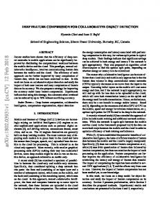
Beyond Filters: Compact Feature Map for Portable Deep Model 15

99.2

81.0

78.0

99.1

99.0

0.04

0.07

0.1

98.9

3 0.01

β

(a) Accuracy of the reconstructed model.

9 6

75.0 0.01

compression speed-up

12

ratio(×)

Accuracy (%)

Accuracy(%)

84.0

0.04

0.07

0.1

0.01

0.04

β

(b) Model accuracy after fine-tuning.

0.07

0.1

β

(c) Compression and speed-up ratios.

Figure 1. The performance of the proposed CNN compression method with different β.

have been discarded since they only account for a subtle proportion of the overall complexity. Hence, considering the major multiplications, the speed-up ratio of the compact network for this layer compared with the original network is di−1 di s2 di−1 di Hi0 Wi0 = . (22) rs = 2i 0 0 ˜ ˜ si di−1 di Hi Wi d˜i−1 d˜i It is obvious that the speed-up ratio for one convolutional layer relates to numbers of filters in this layer and the previous layer. Thus, if we only keep 1/2 filters per layer, the speed-up ratio will be increased to 4×. Compression ratio. The online memory can be divided into two major parts, feature maps of different layers and filters of convolutional layers. Although we can remove feature maps of a layer after it has already been used for calculating the following layer, the the memory allocation and release will increase the time consumption. Moreover, if a layer is connected with several other convolutional layers, we have to store feature maps of previous layers when doing online inference (e.g., the second convolutional layer and the fifth convolutional layer will be combined in ResNet-50 (He et al., 2015), and we have to preserve these feature maps before merging them). For a given convolutional layer Li , the compression ratio of the proposed method is rc =

s2i di−1 di + di Hi0 Wi0 , s2i d˜i−1 d˜i + d˜i Hi0 Wi0

(23)

which is simultaneously affected by the current layer and the pervious layer. Meanwhile, the memory for storing feature maps of other layers, such as pooling layers and Relu layers, will be reduced. We will further illustrate the detailed compression ratio and speed-up ratio of the proposed method in the following section experimentally.

6. Experiments Baselines and Models. Several effective approaches for compressing deep neural networks were selected for comparison: SVD (Denton et al., 2014), XNOR-Net (Rastegari

et al., 2016), Pruning (Han et al., 2016), Perforation (Figurnov et al., 2016), and CNNpack (Wang et al., 2016), and we denoted the proposed method as RedCNN. The evaluation was conducted on the MNIST and ILSVRC2012 datasets (Russakovsky et al., 2015). We first tested the performance of the proposed method and analyzed impacts of parameters on the MNIST dataset using LeNet (LeCun et al., 1998), then compared the proposed method with two benchmark CNNs (VGGNet-16 (Simonyan & Zisserman, 2015) and ResNet-50 (He et al., 2015)) on the ILSVRC 2012 dataset (Russakovsky et al., 2015) which has more than 1 million nature images. All methods were implemented using MatConvNet (Vedaldi & Lenc, 2015) and ran on NVIDIA K40 cards. Filters and data in CNNs were stored and calculated as 32 bit floating-point values. Impact of parameters. The hyper-parameter γ in the proposed reconstruction method (Alg. 1) controls the weight decay regularization and makes weights in new convolution filters not too large. We set γ as 0.0005 empirically. In addition, the proposed dimensionality method (Fcn. 9) has two hyper-parameters, i.e., α and β. We first tested their impact on the network accuracy by conducting an experiment using a LeNet for classifying the MNIST dataset (Vedaldi & Lenc, 2015), where the network has four convolutional layers of size 5 × 5 × 1 × 20, 5 × 5 × 20 × 50, 4 × 4 × 50 × 500, and 1 × 1 × 500 × 10, respectively, and its accuracy is 99.2%. α is used for enforcing the projection matrix P to be orthogonal and is set to be 1.5, experimentally. β is directly related to the sparsity of P , and it effects compression and speed-up ratios of the proposed method. Although a larger β will produce a smaller network, it also leads to a larger distortion on the Euclidean distances between samples. To have a clear illustration, we reported the compression performance by ranging different β, as shown in Fig. 1. From Fig. 1 (a), we found that the compact network reconstructed by using Alg. 1 can also hold a considerable accuracy (e.g., 78% when β = 0.06), which demonstrates that the proposed method can preserve the intrinsic information of the original CNN. Moreover, the accuracy decline can be rebounded (98.9% when β = 0.06) after fine-tuning as


shown in Fig. 1 (b). However, a network that was directly trained with such a small architecture can only achieve a 92.8% accuracy. In addition, although the impact of β is sensitive but monotonous, a larger β enhances compression and speed-up ratios simultaneously, but decreases the accuracy of CNNs as well. The value of β can be easily adjusted according to the demand and restrictions of devices. In our experiments, we set β = 0.06 which provides the best trade-off between compression performance and accuracy, i.e., rc = 11.3×, rs = 8.7×, with 99.16% accuracy. In this case, the layers in the compact convolution network is of the size 5×5×1×5, 5×5×5×20, 4×4×20×96, and 1×1×96×10, respectively. The resulting compact network only occupies around 130KB memory. The MATLAB file of the compressed network and the demo code can be found in https://github.com/YunheWang/RedCNN. Deep Neural Networks Compression on ISLVRC-2012. We next employed the proposed RedCNN for CNN compression on the ImageNet ILSVRC-2012 dataset (Russakovsky et al., 2015), which contains over 1.2M training images and 50k validation images. We evaluated the compression performance on three widely used models: AlexNet (Krizhevsky et al., 2012), which has more than 61M parameters and a top-5 accuracy of 80.8%; VGGNet16 (Simonyan & Zisserman, 2015), which has over 138M parameters and a top-5 accuracy of 90.1%; and ResNet50 (He et al., 2015) which has more than 150 layers with 54 convolutional layers, and a top-5 accuracy of 92.9%. It is worth mentioning that there are considerable filters in the ResNet-50, and thus the network has less redundancy and it is hard for further compression. We first begin our experiment with the AlexNet dataset, and the detailed experimental results were shown in Tab. 1. Table 1. Compression statistics for AlexNet. Layer conv1 conv2 conv3 conv4 conv5 fc6 fc7 fc8 Total

Memory 1.24MB 1.88MB 3.62MB 2.78MB 1.85MB 144MB 64.02MB 15.63MB 235.03MB

rc 2.4× 10.0× 15.5× 3.0× 1.2× 3.5× 72.0× 23.4× 5.06×

Mult. 1.05×108 2.23×108 1.49×108 1.12×108 0.74×108 0.37×108 0.16×108 0.04×108 7.24×108

rs 2.4× 15.4× 21.2× 3.6× 1.2× 3.5× 72.1× 23.5× 4.31×

From Tab. 1, we found that the proposed method achieved a 5.1× compression ratio and a 4.3× speed-up ratio for AlexNet. Then, we reported the compression result of VGGNet-16 in Tab. 2. It can be seen from Tab. 2, we obtained a 6.19× compression ratio and a 9.63× speed-up ratio on VGGNet-16. In addition, the compression ratio and the speed-up ratio on ResNet-50 are 4.14× and 5.82×, respectively. Note that the compression ratio we reported here is calculated by

Table 2. Compression statistics for VGG-16 Net. Layer conv1 1 conv1 2 conv2 1 conv2 2 conv3 1 conv3 2 conv3 3 conv4 1 conv4 2 conv4 3 conv5 1 conv5 2 conv5 3 fc6 fc7 fc8 Total

Memory 12.26MB 12.39MB 6.41MB 6.69MB 4.19MB 5.31MB 5.31MB 6.03MB 10.53MB 10.53MB 9.38MB 9.38MB 9.38MB 392MB 64MB 15.62MB 579.46MB

rc 10.7× 1.8× 3.3× 4.0× 7.2× 2.7× 2.9× 41.3× 16.5× 3.9× 7.8× 18.5× 23.4× 8.6× 3.3× 2.2× 6.19×

Mult. 0.11×109 2.41×109 1.20×109 2.41×109 1.20×109 2.41×109 2.41×109 1.20×109 2.41×109 2.41×109 0.60×109 0.60×109 0.60×109 0.41×109 0.16×108 0.41×107 2.04 × 1010

rs 10.7× 19.0× 5.7× 12.0× 21.9× 10.2× 4.2× 56.2× 70.1× 5.1× 8.0× 21.3× 26.7× 8.6× 3.3× 2.2× 9.63×

Fcn. 23, which contains both convolution filters and feature maps. More compression results of these three CNN models can be found in the supplementary material. Comparison with state-of-the-art methods. Tab. 3 details the compression results of the proposed method and several state-of-the-art methods on three benchmark deep CNN models. Since comparison methods do not change the number of filters of the original neural network, feature map compression ratios of these methods are both equal to 1. Thus, we reported the compression ratio of filters rc1 and feature maps rc2 separately for a fair comparison. For a convolutional neural network with layers, its compression ratios is calculated as Pp Pp 2 0 0 i=1 si di−1 di i=1 di Hi Wi rc1 = Pp . (24) , r = P c 2 p 2˜ ˜ 0 0 ˜ i=1 si di−1 di i=1 di Hi Wi Tab. 3 also shows the cost of various models for processing one image, i.e., storage of filters, memory usage of feature maps, and multiplications for calculating convolutions. It is obvious that feature maps accounting a considerable proportion of memory usage of the whole network, and the proposed RedCNN can provide significant compression ratios rc2 on every network. Although we can remove the feature map of a layer after calculation for saving memory, frequently allocating and releasing is also time consuming. It can be seen from Tab. 3, RedCNN clearly achieves the best performance in terms of both the speed-up ratio (rs ) and the feature map compression ratio (rc1 ). In addition, convolution filter compression ratios of the proposed method is lower than those of pruning (Han et al., 2016) and CNNpack (Wang et al., 2016). These two comparison methods employed quantization approaches (i.e., onedimensional k-means clustering), and thus 32-bit floating values can be converted into about 8-bit values without af-

Beyond Filters: Compact Feature Map for Portable Deep Model Table 3. An overall comparison of state-of-the-art methods for deep neural network compression and speed-up, where rc1 is the compression ratio of convolution filters, rc2 is the compression ratio of feature maps, and rs is the speed-up ratio. Model

AlexNet Filters (232 MB) Maps (2.5MB) Multiplications (7.24 × 108 )

VGGNet-16 Filters (572 MB) Maps (52 MB) Multiplications (1.54 × 1010 )

ResNet-50 Filters (97 MB) Maps (40 MB) Multiplications (5.82 × 109 )

Evaluation rc1 rc2 rs top-1 err top-5 err rc1 rc2 rs top-1 err top-5 err rc1 rc2 rs top-1 err top-5 err

Original 1× 1× 1× 41.8% 19.2% 1× 1× 1× 28.5% 9.9% 1× 1× 1× 24.6% 7.7%

SVD 5× 1× 2× 44.0% 20.5% -

XNOR 32× 32× 64× 56.8% 31.8% -

Pruning 35× 1× 42.7% 19.7% 49× 1× 3.5× 31.1% 10.9% -

Perforation 1.7× 1× 2× 44.7% 1.7× 1× 1.9× 31.0% -

CNNpack 39× 1× 25× 41.6% 19.2% 46× 1× 9.4× 29.7% 10.4% 12.2× 1× 4× 7.8%

RedCNN 5.12× 2.45× 4.31× 42.1% 19.3% 6.87× 3.07× 9.63× 29.3% 10.2% 4.35× 3.71× 5.82× 25.7% 8.2%

fecting the accuracy of the original network. If we adopt this similar strategy, the convolution filter compression ratio rc1 of the proposed scheme can be further multiplied a factor of around 4×, e.g., we can obtain an almost 17.4× filter compression ratio on ResNet-50 model, which is superior to all the other comparison methods. However, 8-bit (or other unconventional format) value cannot be directly used in generic devices (e.g., GPU cards, mobile phones), and thus we did not try them in the experiments of this paper. In summary, the proposed RedCNN can achieve considerable compression and speed-up ratios, which can make existing deep models portable.

were significantly reduced. The results are extremely encouraging, e.g., the compressed ResNet can recognize over 500 images per second. This efficiency can also be inherited into the fine-tuning process, therefore, the compressed networks can be quickly adjusted when applied them to a new dataset. In addition, the practical speed-up ratios of runtimes were slightly lower than the corresponding theoretical speed-up ratios rs due to the costs incurred by data transmission, pooling, padding, etc.. Note that, the runtime reported here is a bit higher than that in (Vedaldi & Lenc, 2015), due to different configurations and hardware environments.

Table 4. Runtime of the proposed deep neural network compression algorithm on different models per image.

7. Conclusions and Discussions

time LeNet AlexNet VGGNet-16 ResNet-50

Original 0.17 ms 1.28 ms 16.67 ms 9.03 ms

RedCNN 0.04 ms 0.74 ms 3.38 ms 1.84 ms

speed-up 4.3× 1.7× 4.9× 4.9×

Runtime. In fact, most of comparison methods cannot significantly accelerate the deep network for various additional operations. For example, (Han et al., 2016) needs to decode the CSR data before testing, which slows down the online inference and will not achieve the comparable compression and speed-up ratios with those of the proposed algorithm in practice. Since the proposed compression method directly re-configures the network into a more compact form, and does not require other additional support for realizing the network speed-up, the runtime of the compressed models for processing images will be reduced significantly. To explicitly demonstrate the superiority of the proposed method, we compared runtimes for recognizing images by benchmark CNN models before and after applying the proposed method, and showed the experimental results in Tab. 4. We found that runtimes of these models after compression

Compression methods for learning portable CNNs are urgently required so that neural networks can be used on mobile devices. Besides convolution filters, the storage of feature maps also accounts for a larger proportion of the online memory usage, we thus no longer search useless connections or weights of filters. In this paper, we present a feature map dimensionality reduction method by excavating and removing redundancy in feature maps generated by different filters. Although the portable network learned by our approach has significantly fewer parameters, its feature maps can also preserve intrinsic information of the original network. Experiments conducted on benchmark datasets and models show that the proposed method can achieve considerable compression ratio and speed-up ratios simultaneously without affecting the classification accuracy of the original CNN. In addition, the compressed network generated by exploiting the proposed method is still a regular CNN with 32-bit float values which does not have any decoding or other procedures for online inference. Acknowledgements We thank supports of NSFC 61375026 and 2015BAF15B00, and ARC Projects: FT-130101457, DP-140102164, LP-150100671.


References Arora, Sanjeev, Bhaskara, Aditya, Ge, Rong, and Ma, Tengyu. Provable bounds for learning some deep representations. ICML, 2014. Bracewell, Ron. The fourier transform and iis applications. New York, 5, 1965. Cheng, Yu, Yu, Felix X, Feris, Rogerio S, Kumar, Sanjiv, Choudhary, Alok, and Chang, Shi-Fu. An exploration of parameter redundancy in deep networks with circulant projections. In CVPR, 2015. Courbariaux, Matthieu and Bengio, Yoshua. Binarynet: Training deep neural networks with weights and activations constrained to+ 1 or-1. arXiv preprint arXiv:1602.02830, 2016.

Liu, Guangcan, Lin, Zhouchen, and Yu, Yong. Robust subspace segmentation by low-rank representation. In ICML, 2010. Long, Jonathan, Shelhamer, Evan, and Darrell, Trevor. Fully convolutional networks for semantic segmentation. In CVPR, 2015. Nie, Feiping, Huang, Heng, Cai, Xiao, and Ding, Chris H. Efficient and robust feature selection via joint `2,1 norms minimization. In NIPS, 2010. Oppenheim, Alan V, Schafer, Ronald W, and Buck, John R. Discrete-time signal processing. Pren- tice Hall Upper Saddle River, 1999. Pan, Zhou and Jiashi, Feng. Outlier-robust tensor pca. In CVPR, 2017.

Denton, Emily L, Zaremba, Wojciech, Bruna, Joan, LeCun, Yann, and Fergus, Rob. Exploiting linear structure within convolutional networks for efficient evaluation. In NIPS, 2014.

Pan, Zhou, Zhouchen, Lin, and Chao, Zhang. Integrated lowrank-based discriminative feature learning for recognition. IEEE TNNLS, 27(5):1080–1093, 2016.

Figurnov, Michael, Vetrov, Dmitry, and Kohli, Pushmeet. Perforatedcnns: Acceleration through elimination of redundant convolutions. NIPS, 2016.

Rastegari, Mohammad, Ordonez, Vicente, Redmon, Joseph, and Farhadi, Ali. Xnor-net: Imagenet classification using binary convolutional neural networks. ECCV, 2016.

Gray, Robert M. Toeplitz and circulant matrices: A review. now publishers inc, 2006.

Ren, Shaoqing, He, Kaiming, Girshick, Ross, and Sun, Jian. Faster r-cnn: Towards real-time object detection with region proposal networks. In NIPS, 2015.

Han, Song, Pool, Jeff, Tran, John, and Dally, William. Learning both weights and connections for efficient neural network. In NIPS, 2015. Han, Song, Mao, Huizi, and Dally, William J. Deep compression: Compressing deep neural networks with pruning, trained quantization and huffman coding. 2016. He, Kaiming, Zhang, Xiangyu, Ren, Shaoqing, and Sun, Jian. Deep residual learning for image recognition. arXiv preprint arXiv:1512.03385, 2015. He, Xiaofei and Niyogi, Partha. Locality preserving projections. In NIPS, 2004. Henriques, Joao F, Martins, Pedro, Caseiro, Rui F, and Batista, Jorge. Fast training of pose detectors in the fourier domain. In NIPS, 2014. Henriques, Jo˜ao F, Caseiro, Rui, Martins, Pedro, and Batista, Jorge. High-speed tracking with kernelized correlation filters. IEEE TPAMI, 37(3):583–596, 2015. Hinton, Geoffrey, Vinyals, Oriol, and Dean, Jeff. Distilling the knowledge in a neural network. arXiv preprint arXiv:1503.02531, 2015. Hu, Hengyuan, Peng, Rui, Tai, Yu-Wing, and Tang, ChiKeung. Network trimming: A data-driven neuron pruning approach towards efficient deep architectures. arXiv preprint arXiv:1607.03250, 2016. Krizhevsky, Alex, Sutskever, Ilya, and Hinton, Geoffrey E. Imagenet classification with deep convolutional neural networks. In NIPS, 2012. LeCun, Yann, Bottou, L´eon, Bengio, Yoshua, and Haffner, Patrick. Gradient-based learning applied to document recognition. Proceedings of the IEEE, 86(11):2278–2324, 1998. Li, Hao, Kadav, Asim, Durdanovic, Igor, Samet, Hanan, and Graf, Hans Peter. Pruning filters for efficient convnets. arXiv preprint arXiv:1608.08710, 2016. Liu, Baoyuan, Wang, Min, Foroosh, Hassan, Tappen, Marshall, and Pensky, Marianna. Sparse convolutional neural networks. In CVPR, 2015.

Romero, Adriana, Ballas, Nicolas, Kahou, Samira Ebrahimi, Chassang, Antoine, Gatta, Carlo, and Bengio, Yoshua. Fitnets: Hints for thin deep nets. In ICLR, 2015. Roweis, Sam T and Saul, Lawrence K. Nonlinear dimensionality reduction by locally linear embedding. Science, 290(5500): 2323–2326, 2000. Russakovsky, Olga, Deng, Jia, Su, Hao, Krause, Jonathan, Satheesh, Sanjeev, Ma, Sean, Huang, Zhiheng, Karpathy, Andrej, Khosla, Aditya, Bernstein, Michael, et al. Imagenet large scale visual recognition challenge. IJCV, 115(3):211– 252, 2015. Simonyan, Karen and Zisserman, Andrew. Very deep convolutional networks for large-scale image recognition. ICLR, 2015. Tenenbaum, Joshua B, De Silva, Vin, and Langford, John C. A global geometric framework for nonlinear dimensionality reduction. science, 290(5500):2319–2323, 2000. Vedaldi, Andrea and Lenc, Karel. Matconvnet: Convolutional neural networks for matlab. In Proceedings of the 23rd Annual ACM Conference on Multimedia Conference, 2015. Wang, Yunhe, Xu, Chang, You, Shan, Tao, Dacheng, and Xu, Chao. Cnnpack: Packing convolutional neural networks in the frequency domain. In NIPS, 2016. Wen, Wei, Wu, Chunpeng, Wang, Yandan, Chen, Yiran, and Li, Hai. Learning structured sparsity in deep neural networks. In NIPS, 2016. Wold, Svante, Esbensen, Kim, and Geladi, Paul. Principal component analysis. Chemometrics and intelligent laboratory systems, 2(1-3):37–52, 1987. Xu, Chang, Tao, Dacheng, Xu, Chao, and Rui, Yong. Largemargin weakly supervised dimensionality reduction. In ICML, 2014.