Dec 20, 2012 - in Section 6, and proofs of the main results are contained in Section 7. ...... Haar wavelets with edge length 2pân satisfying |he n,l(t1,t2 + 1) â he.
Beyond incoherence: stable and robust sampling strategies for compressive imaging Felix Krahmer and Rachel Ward December 20, 2012
Abstract In many signal processing applications, one wishes to acquire images that are sparse in transform domains such as spatial finite differences or wavelets using frequency domain samples. For such applications, overwhelming empirical evidence suggests that superior image reconstruction can be obtained through variable density sampling strategies that concentrate on lower frequencies. The wavelet and Fourier transform domains are not incoherent because low-order wavelets and low-order frequencies are correlated, so compressed sensing theory does not immediately imply sampling strategies and reconstruction guarantees. In this paper we turn to a more refined notion of coherence – the so-called local coherence – measuring for each sensing vector separately how correlated it is to the sparsity basis. For Fourier measurements and Haar wavelet sparsity, the local coherence can be controlled, so for matrices comprised of frequencies sampled from suitable power-law densities, we can prove the restricted isometry property with near-optimal embedding dimensions. Consequently, the variable-density sampling strategies we provide — which are independent of the ambient dimension up to logarithmic factors — allow for image reconstructions that are stable to sparsity defects and robust to measurement noise. Our results cover both reconstruction by `1 -minimization and by total variation minimization.
1
Introduction
The measurement process in a wide range of imaging applications such as radar, sonar, astronomy, and computer tomography, can be modeled – after appropriate approximation and discretization – as taking samples from weighted discrete Fourier transforms [16]. Similarly, it is well known in the medical imaging literature that the measurements taken in Magnetic Resonance Imaging (MRI) are well modeled as Fourier coefficients of the desired image. Within all of these scenarios, one seeks strategies for taking frequency domain measurements so as to reduce the number of measurements without degrading the quality of image reconstruction. A central feature of natural images that can be exploited in this process is that they allow for approximately sparse representation in suitable bases or dictionaries. 1
The theory of compressed sensing, also termed compressive sampling, as introduced in [14, 8], fits comfortably into this set-up: its key observation is that signals which allow for a sparse or approximately sparse representation can be recovered from relatively few linear measurements via convex approximation, provided these measurements are sufficiently incoherent with the basis in which the signal is sparse.
1.1
Imaging with partial frequency measurements
Much work in compressed sensing has focused on the setting of imaging with frequency domain measurements [8, 7, 34] and, in particular, towards accelerating the MRI measurement process [22, 21]. For images that are localized in the pixel domain, the incoherence between pixel and Fourier bases implies that uniformly subsampled discrete Fourier transform measurements can be used to achieve near-optimal oracle reconstruction bounds: up to logarithmic factors in the discretization size, any image can be approximated from s such frequency measurements up to the error that would be incurred if the image were first acquired in full, and then compressed by setting all but the s largest-magnitude pixels to zero [34, 31, 7, 9]. Compressed sensing recovery guarantees hold more generally subject to incoherence between sampling and sparsity transform domains. Unfortunately, natural images are generally not directly sparse in the pixel basis, but rather with respect to transform domains more closely resembling wavelet bases. As low-scale wavelets are highly correlated (coherent) with low frequencies, sampling theorems for compressive imaging with partial Fourier transform measurements have remained elusive. A number of empirical studies, including the very first papers on compressed sensing MRI [22, 21], suggest that better image restoration is possible by subsampling frequency measurements from variable densities preferring low frequencies to high frequencies. In fact, variable-density MRI sampling had been proposed previously in a number of works outside the context of compressed sensing, although there did not seem to be a consensus on an optimal density [23, 36, 38, 28, 18]. For a thorough empirical comparison of different densities from the compressed sensing perspective, see [39]. Guided by these observations, the authors of [30] estimated the coherence between each element of the sensing basis with elements of the sparsity basis separately as a means to derive optimal sampling strategies in the context of compressed sensing MRI. In particular, they observe that incoherence-based results in compressed sensing imply exact recovery results for more general systems if one samples a row from the measurement basis proportionally to its squared maximal correlation with the sparsity-inducing basis. For given problem dimensions, they find the optimal distribution as the solution to a convex problem. In [29], the approach of optimizing the sampling distribution is combined with premodulation by a chirp, which by itself is another measure to reduce the coherence [3, 20]. A similar variable-density analysis already appeared in [33] in the context of sampling strategies and reconstruction guarantees for functions with sparse orthogonal polynomial expansions and will also be the guiding strategy of this paper (cf. Section 5).
2
1.2
Contributions of this paper
In this paper we derive near-optimal reconstruction bounds for variable-density subsampled discrete Fourier transform measurements for both wavelet sparsity and gradient sparsity models. More precisely, up to logarithmic factors in the discretization size, any image can be approximated from s such measurements up to the error that would be incurred if the wavelet transform or the gradient of the image, respectively, were first computed in full, and then compressed by setting all but the s largest-magnitude coefficients to zero. Note that the reconstruction results that have been derived for uniformly-subsampled frequency measurements [8, 15] are not optimal in this sense. A major role in determining the best sampling density will be played by the local coherence of the sensing basis with respect to the sparsity basis, as introduced in Section 5. Consequently, an important ingredient of our analysis is Theorem 6.2, which provides frequency-dependent bounds on inner products between rows of the orthonormal discrete Fourier transform and rows of the orthonormal discrete Haar wavelet transform. In particular, the maximal correlation between a fixed row in the discrete Fourier transform and any row of the discrete Haar wavelet transform decreases according to an inverse power law of the frequency, and decays sufficiently quickly that the sum of squared maximal correlations scales only logarithmically with the discretization size N . This implies, according to the techniques used in [33, 32, 4], that subsampling rows of the discrete Fourier matrix proportionally to the squared correlation results in a matrix that has the restricted isometry property of near-optimal order subject to appropriate rescaling of the rows. For reconstruction, total variation minimization [35, 5, 27, 37, 11, 10] will be our algorithm of choice. In the papers [25] and [26], total variation minimization was shown to provide stable and robust image reconstruction provided that the sensing matrix is incoherent with the Haar wavelet basis. Following the approach of [25], we prove that from variable density frequency samples, total variation minimization can be used for stable image recovery guarantees. Due to the effects of variable density sampling we will no longer need the samples to be incoherent to the Haar basis.
1.3
Outline
The remainder of this paper is organized as follows. Preliminary notation is introduced in Section 2. The main results of this paper along with a numerical illustration are contained in Section 3. Section 4 reviews compressed sensing theory and Section 5 presents recent results on sampling strategies for coherent systems. The main results on the coherence between Fourier and Haar wavelet bases is provided in Section 6, and proofs of the main results are contained in Section 7. We conclude with a summary and a discussion of open problems in Section 8.
3
2
Preliminaries
2.1
Notation
In this paper, we consider discrete images, that is, N × N blocks of pixels, and represent them as discrete functions f ∈ CN ×N . We write f (t1 , t2 ) to denote any particular pixel value and for a positive integer N , we denote the set {1, 2, . . . , N } by [N ]. By f1 ◦ f2 we denote the Hadamard product, i.e., the image resulting from pointwise products of the pixel values, f1 ◦ f2 (t1 , t2 ) = f1 (t1 , t2 )f2 (t1 , t2 ). On the space � P p 1/p , 1 ≤ p < ∞, and kf k∞ = of such images, the `p vector norm is given by kf kp = t1 ,t2 |f (t1 , t2 )| P max(t1 ,t2 ) |f (t1 , t2 )|. The inner product inducing the `2 vector norm is hf, gi = t1 ,t2 f¯(t1 , t2 )g(t1 , t2 ), where z¯ denotes the complex conjugate of number z ∈ C. By an abuse of notation, the “`0 -norm” kf k0 = #{(t1 , t2 ) : f (t1 , t2 ) 6= 0} counts the number of non-zero entries of f . An image f is called s-sparse if kf k0 ≤ s. The error of best s-term approximation of an image f in `p is defined as σs (f )p =
inf
g:kgk0 ≤s
kf − gkp .
Clearly, σs (f )p = 0 if f is s-sparse. Informally, f is called compressible if σs (f )1 decays quickly as s increases. For two nonnegative functions f (t) and g(t) on the real line, we write f & g (or f . g) if there exists a constant C > 0 such that f (t) ≥ Cg(t) (or f (t) ≤ Cg(t), respectively) for all t > 0. The discrete directional derivatives of f ∈ CN ×N are defined pixel-wise as
fx ∈ CN −1×N ,
fx (t1 , t2 )
= f (t1 + 1, t2 ) − f (t1 , t2 )
fy ∈ CN ×N −1 ,
fy (t1 , t2 )
= f (t1 , t2 + 1) − f (t1 , t2 )
The discrete gradient transform ∇ : CN ×N → CN ×N ×2 is defined in terms of the directional derivatives via � � ∇f (t1 , t2 ) := fx (t1 , t2 ), fy (t1 , t2 ) ,
where the directional derivatives are extended to N × N by adding zero entries. The total variation semi-norm is the `1 norm of the image gradient,
kf kT V := k∇f k1 =
X
� |fx (t1 , t2 )| + |fy (t1 , t2 )| .
t1 ,t2
Here we note that our definition is the anisotropic version of the total variation semi-norm. The
4
isotropic total variation semi-norm becomes the sum of terms � fx (t1 , t2 ) + ify (t1 , t2 ) = fx (t1 , t2 )2 + fy (t1 , t2 )2 1/2 .
The isotropic and anisotropic total variation semi-norms are thus equivalent up to a factor of
2.2
√
2.
Bases for sparse representation and measurements
The Haar wavelet basis is a simple basis which allows for good sparse approximations of natural images. We will work primarily in two dimensions, but first introduce the univariate Haar wavelet basis as it will nevertheless serve as a building block for higher dimensional bases. Definition 2.1 (Univariate Haar wavelet basis). The univariate discrete Haar wavelet system is an p
orthonormal basis of C2 consisting of the constant function h0 (t) ≡ 2−p/2 , the step function h10,0 = h1 given by h1 (t) =
2−p/2 ,
1 ≤ t ≤ 2p−1 ,
−2−p/2 , 2p−1 < t ≤ 2p , along with the dyadic step functions n
h1n,` (t) = 2 2 h1 (2n t − `) n−p 2 2 for = −2 n−p 2 for 0 else,
`2p−n ≤ t < `2p−n + 2p−n−1 `2p−n + 2p−n−1 ≤ t < `2p−n + 2p−n
for (n, `) ∈ Z2 satisfying 0 < n < p and 0 ≤ ` < 2n . p
To define the bivariate Haar wavelet basis of C2
×2p
, we extend the univariate system by the window
functions
n
h0n,` (t) = 2 2 h0 (2n t − `) =
n−p 2 2
for
0
else.
`2p−n ≤ t < (` + 1)2p−n
The bivariate Haar wavelet system can now be defined via tensor products of functions in the extended p
univariate system. In order for the system to form an orthonormal basis of C2
×2p
, only tensor products
of univariate functions with the same scaling parameter n are included. p
Definition 2.2 (Bivariate Haar wavelet basis). The bivariate Haar system of C2
5
×2p
consists of the
constant function h(0,0) given by
h(0,0) (t1 , t2 ) = h0 (t1 )h0 (t2 ) ≡ 2−p
and the functions hen,` with indices in the range 0 ≤ n < p, ` = (`1 , `2 ) ∈ Z2 ∩ [0, 2n )2 , and � e = (e1 , e2 ) ∈ {0, 1}, {1, 0}, {1, 1} given by 1 2 hen,` (t1 , t2 ) = hen,` (t1 )hen,` (t2 ). 1 2
We denote by H the bivariate Haar transform f → hf, hn,` i
� n,`
and, by a slight abuse of notation, also
the unitary matrix representing this linear map. We will also work with discrete Fourier measurements. Definition 2.3 (Discrete Fourier basis). Let N = 2p . The one-dimensional discrete Fourier system is an orthonormal basis of CN consisting of the vectors 1 ϕk (t) = √ ei2πtk/N , N
−N/2 + 1 ≤ t ≤ N,
indexed by discrete frequencies in the range −N/2 + 1 ≤ k ≤ N/2. The two-dimensional discrete Fourier basis of CN ×N is just a tensor product of one-dimensional bases, namely
ϕk1 ,k2 (t1 , t2 ) =
1 i2π(t1 k1 +t2 k2 )/N e , N
−N/2 + 1 ≤ t1 , t2 ≤ N/2,
(2.3)
indexed by discrete frequencies in the range −N/2 + 1 ≤ k1 , k2 ≤ N/2. We denote by F the two-dimensional discrete Fourier transform f → hf, ϕk1 ,k2 i
� k1 ,k2
and, again, also
the associated unitary matrix. Finally, we denote by FΩ its restriction to a set of frequencies Ω ⊂ [N ]2 .
3
Main results
Our main results say that appropriate variable density subsampling of the discrete Fourier transform will with high probability result in a set of measurements admitting stable image reconstruction via total variation minimization or `1 -minimization. While our recovery guarantees are robust to measurement noise, the model we consider corresponds to a weighted `2 -norm such that high-frequency measurements have higher sensitivity to noise. Loosely speaking, this compensates for the smaller number of samples in regions of low sampling probability. Our first result concerns stable recovery guarantees for total variation minimization.
6
Theorem 3.1. Fix integers N = 2p , m, and s such that s & log(N ) and m & s log3 (s) log5 (N ).
2 Select m frequencies {(ω1j , ω2j )}m j=1 ⊂ {−N/2 + 1, . . . , N/2} i.i.d. according to
� � j j � Prob (ω1 , ω2 ) = (k1 , k2 ) = CN min C,
1 2 k1 + k22
� =: η(k1 , k2 ),
−N/2 + 1 ≤ k1 , k2 ≤ N/2,
(3.1)
where C is an absolute constant and CN is chosen such that η is a probability distribution. j 1/2 j , and assume that the noise vector Consider the weight vector ρ = (ρj )m j=1 with ρj = (1/η(ω1 , ω2 )) √ −C log3 (s) ξ = (ξj )m , j=1 satisfies kρ ◦ ξk2 ≤ ε m, for some � > 0. Then with probability exceeding 1 − N
the following holds for all images f ∈ CN ×N : Given noisy partial Fourier measurements y = FΩ f + ξ, the estimation f # = argmin kgkT V
such that
√ kρ ◦ (FΩ g − y)k2 ≤ ε m,
(3.2)
g∈CN ×N
approximates f up to the noise level and best s-term approximation error of its gradient:
kf − f # k2 .
k∇f − (∇f )s k1 √ + ε. s
Disregarding measurement noise, the error rate provided in Theorem 3.1 (and also the one in Theorem 3.2 below) is optimal up to logarithmic factors in the ambient image dimension. This follows from classical results about the Gel’fand width of the `1 -ball due to Kashin [19] and Garnaev–Gluskin [17]. Numerical results such as those detailed in [39] and illustrated below in Figure 1 confirm that variabledensity sampling strategies significantly outperform uniform sampling strategies as well as deterministic sampling strategies, and Theorem 3.1 provides theoretical justification for such observations. Our second result focuses on stable image reconstruction by `1 -minimization in the Haar wavelet transform domain. It is a direct consequence of applying the Fourier-wavelet incoherence estimates derived in Theorem 5.2 to Theorem 6.2. Theorem 3.2. Fix integers N = 2p , m, and s such that s & log(N ) and m & s log2 (N ) log3 (s).
2 Select m frequencies Ω = {(ω1j , ω2j )}m j=1 ⊂ {−N/2 + 1, . . . , N/2} i.i.d. according to the density η as in
(3.1) and assume again that the noise vector ξ = (ξj )m j=1 satisfies the weighted `2 -constraint with weight ρ and noise level ε as in Theorem 3.1. Then with probability exceeding 1 − N −C log 7
3
(s)
, the following holds
for all images f ∈ CN ×N : Given noisy measurements y = FΩ f + ξ, the estimation f # = argmin kHgk1
such that
√ kρ ◦ (FΩ g − y)k2 ≤ ε m
g∈CN ×N
approximates f up to the noise level and best s-term approximation error in the bivariate Haar basis:
kf − f # k2 .
kHf − (Hf )s k1 √ + ε. s
Even though the required number of samples m in Theorem 3.2 is smaller than the number of samples required for the total variation minimization guarantees in Theorem 3.1, we find that total variation minimization requires fewer measurements empirically. This may be due to the fact that the gradient of a natural image has stronger sparsity than its Haar wavelet representation. For this reason we focus on total variation minimization. Independent of this observation, we strongly suspect that the additional logarithmic factors in the number of measurements stated in Theorem 3.1 are an artifact of the proof, and that it should be possible to strengthen the result to obtain a similar recovery guarantee with the number of measurements as in Theorem 3.2.
4 4.1
Compressed sensing background The restricted isometry property
Under very mild assumptions on the matrix Φ : CN → Cm , any k-sparse x ∈ CN can be recovered from y = Φx as the solution to the optimization problem:
x = argmin kzk0
such that
Φz = y
One of the fundamental results in compressed sensing is that this optimization problem, which is NP-hard in general, can be relaxed to an `1 -minimization problem if one asks that the matrix Φ restricted to any subset of 2k columns be well-conditioned. This property is quantified via the so-called restricted isometry property as introduced in [9]: Definition 4.1 (Restricted isometry property). Let Φ ∈ Cm×N . For s ≤ N , the restricted isometry constant δs associated to Φ is the smallest number δ for which (1 − δ)kxk22 ≤ kΦxk22 ≤ (1 + δ)kxk22 for all s-sparse vectors x ∈ CN . If δs ≤ δ, one says that Φ has the restricted isometry property (RIP) of 8
order s and level δ. The restricted isometry property ensures stability: not only sparse vectors, but also compressible vectors can be recovered from the measurements via `1 -minimization. It also ensures robustness to measurement errors. Proposition 4.2 (Sparse recovery for RIP matrices). Assume that the restricted isometry constant δ5s of Φ ∈ Cm×N satisfies δ5s < 13 . Let x ∈ CN and assume noisy measurements y = Φx + ξ with kξk2 ≤ ε. Then
x# = arg min
z∈CN
kzk1 subject to
kΦz − yk2 ≤ ε
satisfies
kx − x# k2 ≤
2σs (x)1 √ + ε. s
In particular, reconstruction is exact, x# = x, if x is s-sparse and ε = 0. There are stronger versions of this result which allow for weaker constraints on the restricted isometry constant [24]. However, our version is a corollary of the following proposition, which generalizes the results from [8] and seem to have appeared first in [25]. This proposition will also play an important role in the proof of our main results. Proposition 4.3 (Stable recovery for RIP matrices, [25]). Suppose that γ ≥ 1 and Φ ∈ Cm×N satisfies the restricted isometry property of order 5kγ 2 and level δ < 1/3, and suppose that u ∈ CN satisfies a tube constraint kΦuk2 . ε. Suppose further that for a subset S of cardinality |S| = k, the signal u satisfies a cone constraint
kuS c k1 ≤ γkuS k1 + ξ.
Then ξ kuk2 . √ + ε. γ k
(4.1)
Proposition 4.2 follows from Proposition 4.3 by noting that the minimality of x# implies a cone constraint for the residual x − x# over the support of the s largest-magnitude entries of x. For completeness, the proof of Proposition 4.3 is recalled in the appendix.
9
4.2
Bounded orthonormal systems
While the strongest known results on the restricted isometry property concern random matrices with independent entries such as Gaussian or Bernoulli, a scenario that has proven particularly useful for applications is that of structured random matrices with rows chosen from a basis incoherent to the basis inducing sparsity (see below for a detailed discussion on the concept of incoherence). The resulting sampling schemes correspond to bounded orthonormal systems, and such systems have been extensively studied in the compressed sensing literature (see [31] for an expository article including many references). Definition 4.4 (Bounded orthonormal system). Consider a set T equipped with probability measure ν. • A set of functions {ψj : T → C, j ∈ [N ]} is called an orthonormal system with respect to ν if R ψ¯ (x)ψk (x)dν(x) = δjk , where δjk denotes the Kronecker delta. T j • An orthonormal system is said to be bounded with bound K if supj∈[N ] kψj (x)k∞ ≤ K.
For example, the basis of complex exponentials ψj (x) = exp (i2πjx) forms a bounded orthonormal system with optimally small constant K = 1 with respect to the uniform measure on T = {0, N1 , . . . , NN−1 }, and d-dimensional tensor products of complex exponentials form bounded orthonormal systems with respect to the uniform measure on the set T d . A random sample of an orthonormal system is the vector (ψ1 (x), . . . , ψN (x)), where x is a random variable drawn according to the associated distribution ν. Any matrix whose rows are independent random samples of a bounded orthonormal system, such as the uniformly subsampled discrete Fourier matrix, will have the restricted isometry property: Proposition 4.5 (RIP for bounded orthonormal systems, [31]). Consider the matrix Ψ ∈ Cm×N whose rows are independent random samples of a orthonormal system {ψj , j ∈ [N ]} with bound K ≥ 1 and orthogonalization measure ν. If m & δ −2 K 2 s log3 (s) log(N ),
for some s & log(N )1 , then with probability at least 1 − N −C log of
√1 Ψ m
3
(s)
, the restricted isometry constant δs
satisfies δs ≤ δ.
An important special case of a bounded orthonormal system arises by sampling a function with sparse representation in one basis using measurements from a different, incoherent basis. The mutual coherence N ×N between a unitary matrix A ∈ CN ×N with rows (aj )N with rows j=1 and a unitary matrix B ∈ C
(bj )N j=1 is given by µ(A, B) = sup | haj , bk i | j,k 1 For matrices consisting of uniformly subsampled rows of the discrete Fourier matrix, it has been shown in [12] that this constraint is not necessary.
10
The smallest possible mutual coherence is µ = N −1/2 , as realized by the discrete Fourier matrix and the identity matrix. We call two orthonormal bases A and B mutually incoherent if µ = O(N −1/2 ) or √ e µ = O(logα (N )N −1/2 ). In this case, the rows (˜bj )N N BA∗ constitute a bounded j=1 of the basis B = orthonormal system with respect to the uniform measure. Propositions 4.5 and 4.2 then imply that, with high probability, signals f ∈ CN of the form f = Ax for x sparse can be stably reconstructed from e as B e has the restricted isometry property. uniformly subsampled measurements y = Bf = Bx, Corollary 4.6 (RIP for incoherent systems, [34]). Consider orthonormal bases A, B ∈ CN ×N with mutual coherence bounded by µ(A, B) ≤ KN −1/2 . Fix δ > 0 and integers N, m, and s such that s & log(N ) and m & δ −2 K 2 s log3 (s) log(N ).
(4.2)
Consider the matrix Φ ∈ Cm×N formed by uniformly subsampling m rows i.i.d. from the the matrix √ e = N BA∗ . Then with probability at least 1 − N −c log3 (s) , the restricted isometry constant δs of √1 Φ B m satisfies δs ≤ δ.
5
Local coherence The coherence-based sparse recovery results implied by Corollary 4.6 do not take advantage of the
full range of applicability of bounded orthonormal systems. As argued in [33], Proposition 4.5 implies comparable sparse recovery guarantees for a much wider class of sampling/sparsity bases through preconditioning resampled systems. In the following, we formalize this approach through the notion of local coherence. N Definition 5.1 (Local coherence). The local coherence of an orthonormal basis {ϕj }N with j=1 of C N respect to the orthonormal basis {ψk }N is the function µloc (Φ, Ψ) ∈ RN defined coordinate-wise k=1 of C
by µloc j (Φ, Ψ) = sup |hϕj , ψk i|. 1≤k≤N
The following result shows that we can reduce the number of measurements m in (4.6) by replacing the bound K on the coherence in (4.2) by a bound on the `2 -norm of the local coherence, provided we sample rows from Φ appropriately using the local coherence function. It can be seen as a direct finite-dimensional analog to Theorem 2.1 in [33], but for completeness, we include a short self-contained proof. N N Theorem 5.2. Let Φ = {ϕj }N j=1 and Ψ = {ψk }k=1 be orthonormal bases of C . Assume the local
coherence of Φ with respect to Ψ is pointwise bounded by the function κ, that is
sup |hϕj , ψk i| ≤ κj . 1≤k≤N
Let s & log(N ), suppose m & δ −2 kκk22 s log3 (s) log(N ),
11
and choose m (possibly not distinct) indices j ∈ Ω ⊂ [N ] i.i.d. from the probability measure ν on [N ] given by ν(j) =
κ2j . kκk22
Consider the matrix A ∈ Cm×N with entries
Aj,k = hϕj , ψk i,
j ∈ Ω, k ∈ [N ],
and consider the diagonal matrix D = diag(d) ∈ CN with dj = kκk2 /κj . Then with probability at least 1 − N −c log
3
(s)
, the restricted isometry constant δs of the preconditioned matrix
√1 DA m
satisfies δs ≤ δ.
Proof. We show that the system {ϕ ej } = {dj ϕj } is an orthonormal system with respect to ν in the sense of Definition 4.4. Indeed, N X
ϕ ej (k1 )ϕ ej (k2 )ν(j) =
j=1
N � X kκk2 j=1
=
N X
κj
�� kκk � κ2 2 j ϕj (k1 ) ϕj (k2 ) κj kκk22
ϕj (k1 )ϕj (k2 ) = δk1 ,k2 ;
j=1
hence the ϕ ej form an orthonormal system with respect to ν. Noting that this system is bounded with bound kκk2 , the result follows from Proposition 4.5. Remark 5.3. Note that the local coherence not only appears in the embedding dimension m, but also in the sampling measure. Hence a priori, one cannot guarantee the optimal embedding dimension if one only has suboptimal bounds for the local coherence. That is why the sampling measure in Theorem 5.2 is defined via the (known) upper bounds κ and kκk2 rather than the (usually unknown) exact values µloc and kµloc k2 , showing that suboptimal bounds still lead to meaningful bounds on the embedding dimension. Remark 5.4. For µ ≤ KN −1/2 (as in Corollary 4.6), one has kµloc k2 ≤ K , so Theorem 5.2 is a direct generalization of Corollary 4.6. As one has equality if and only if µloc is constant, however, Theorem 5.2 will be stronger in most cases.
6
Local coherence estimates for frequencies and wavelets Due to the tensor product structure of both of these bases, the two-dimensional local coherence of the
two-dimensional Fourier basis with respect to bivariate Haar wavelets will follow by first bounding the local coherence of the one-dimensional Fourier basis with respect to the set of univariate building block functions of the bivariate Haar basis.
12
Lemma 6.1. Fix N = 2p with p ∈ N. For the space CN , the one-dimensional Fourier basis vectors ϕk , k 6= 0, and the one-dimensional Haar wavelet basis building blocks hen,k , e = 0, 1, satisfy the incoherence relation |hϕk , hen,` i|
≤ min
� 6 · 2 n2 |k|
� n , 3π2− 2 .
Proof. We estimate
hϕk , hen,` i
=
p−n−1 2p−n `+2 X −1
2
n−p 2
−p −p kj 2 2πi2
2
e
+ (−1)
−n
`k
�
`k
�
p−n 2p−n `+2 X −1
2
n−p 2
p
−p
2− 2 e2πi2
kj
j=2p−n `+2p−n−1
j=2p−n `
= e2πi2
e
−n−1
1 + (−1)e e2πi2
k
�
k
�
n
2 2 −p
2p−n−1 X −1
−p
e2πi2
kj
j=0 −n−1
−n
= e2πi2
−n−1
1 + (−1)e e2πi2
n
2 2 −p
k 1 − e2πi2 −p k . 2πi2 1−e
To estimate this expression, we note that −n−1
|1 − e2πi2
k
| ≤ min(2, π2−n |k|)
(6.1)
and distinguish two cases: −p
If 0 6= |k| ≤ 2p−2 , we bound |1 − e2πi2
k
| ≥ 2−p |k| and apply (6.1) to obtain min(2, π2−n |k|) 2−p |k| n n 4 · 22 ≤ min( , 2π2− 2 ). |k| n
|hϕk , hen,` i| ≤ 2 · 2 2 −p
−p
For 2p−2 < |k| ≤ 2p−1 , and hence 2−p ≤ 21 |k|−1 , we note that |1 − e2πi2
k
√
|≥
2 2
and bound, again using
(6.1), n
|hϕk , hen,` i| ≤ 2 · 2 2 |k|−1 ≤ min
min(2, π2−n |k|)
� 6 · 2 n2 |k|
√
2 2
� n , 3π2− 2 .
This lemma enables us to derive the following incoherence estimates for the bivariate case. Theorem 6.2. Let N = 2p for N 3 p ≥ 8. Then the local coherence µloc of the orthonormal twodimensional Fourier basis {ϕk1 ,k2 } with respect to the orthonormal bivariate Haar wavelet basis {hen,` } in
13
CN ×N , as defined in (2.3) and (2.2), respectively, is bounded by � 18π ≤ κ(k1 , k2 ) := min 1, max(|k1 |, |k2 |) ! √ 18π 2 ≤ κ0 (k1 , k2 ) := min 1, , 1/2 (|k1 |2 + |k2 |2 ) �
µloc k1 ,k2
p √ and one has kκk2 ≤ kκ0 k2 ≤ 52 p = 52 log2 (N ). Proof. First note that the bivariate Fourier coefficients decompose into the product of univariate Fourier coefficients:
1 2 hϕk1 ,k2 , hen,` i = hϕk1 , hen,` ihϕk2 , hen,` i. 1 2
For ki 6= 0, the factors can be bounded using Lemma 6.1, which, for k1 6= 0 6= k2 , yields the bound |hϕk1 ,k2 , hen,` i| ≤ min
� � 6 · 2 n2 � n n 18π , 3π2− 2 min , 3π2− 2 ≤ . |k1 | |k2 | max(|k1 |, |k2 |)
� 6 · 2 n2
Next we consider the case where either k1 = 0 or k2 = 0; w.l.o.g., assume k1 = 0. We use that in one n
dimension, we have hϕ0 , h1n,` i = 0 as well as hϕ0 , h0n,` i = 2− 2 . So we only need to consider the case that e1 = 0 and hence e2 = 1. Thus we obtain n
n
|hϕ0,k2 , hen,` i| ≤ 2− 2 In both cases, we obtain µloc k1 ,k2 ≤
18π max(|k1 |,|k2 |) .
6 · 22 6 = . |k2 | max(|k1 |, |k2 |)
The bound µloc k1 ,k2 ≤ 1 follows directly from the Cauchy-
0 Schwartz inequality. We conclude µloc k1 ,k2 ≤ κ(k1 , k2 ) ≤ κ (k1 , k2 ).
For the `2 -bound, we use an integral estimate,
kκ0 k22
≤ #{(k1 , k2 ) :
k12
+
k22
p−1 2X
2
≤ 648π } +
k1 ,k2 =−2p−1 +1 |k1 |2 +|k2 |2 >648π 2
648π 2 |k1 |2 + |k2 |2
1
p− 2Z Z2
≤ 20600 +
√ 18π 2r−1 drdφ
√ r=18π 2−1
≤ 17200 + 502 log2 (N ) ≤ 2700 log2 (N ) = 2700p,
where we used that p ≥ 8. Taking square root implies the result. As the infimum of a strictly decreasing function and a strictly increasing function is bounded uniformly by its value at the intersection point of the two functions, Lemma 6.1 also gives frequency-dependent bounds for the local coherence between frequencies and wavelets in the univariate setting. 14
Corollary 6.3. Fix N = 2p with p ∈ N. For the space CN , the one-dimensional Fourier basis vectors ϕk , k 6= 0, and the one-dimensional Haar wavelets satisfy the incoherence relation √ √ |hϕk , hn,` i| ≤ 3 2π/ k.
7
Recovery guarantees
7.1
Proof of Theorem 3.2
The proof of Theorem 3.2 concerning recovery from `1 -minimization in the bivariate Haar transform domain follows by combining the local incoherence estimate of Theorem 6.2 with the local coherence based reconstruction guarantees of Theorem 5.2. Under the conditions of Theorem 5.2, the stated recovery results follow directly from Theorem 4.2. The weighted `2 -norm in the noise model is a consequence of the preconditioning.
7.2
Preliminary lemmas for the proof of Theorem 3.1
The proof of Theorem 3.1 proceeds along similar lines to that of Theorem 3.2, but we need a few more preliminary results relating the bivariate Haar transform to the gradient transform. Each of the following results are derived from a more general statement involving the continuous bivariate Haar system and the bounded variation seminorm. 2
Proposition 7.1. Suppose f ∈ CN , and suppose its bivariate Haar transform w = Hf ∈ CN
2
is
arranged such that w(k) is the k-th largest-magnitude coefficient. Then there is a universal constant C > 0 such that for all k ≥ 1, |w(k) | ≤ C
kf kT V k
In words, this proposition says that the bivariate Haar coefficient sequence of a function f is in weak `1 and its weak `1 semi-norm is bounded by the total variation semi-norm of f . See [25] for a derivation of Proposition 7.1 from Theorem 8.1 of [13]. We also have the following result about the bivariate Haar system. Lemma 7.2. Let N = 2p . For any indices (t1 , t2 ) and (t1 , t2 + 1), there are at most 6p bivariate Haar wavelets hen,` satisfying |hen,` (t1 , t2 + 1) − hen,` (t1 , t2 )| > 0. Proof. The lemma follows by showing that for fixed dyadic scale n in 0 < n ≤ p, there are at most 6 Haar wavelets with edge length 2p−n satisfying |hen,` (t1 , t2 + 1) − hen,` (t1 , t2 )| > 0. If the edge between (t1 , t2 ) and (t1 , t2 + 1) coincides with a dyadic edge at scale n, then the 3 wavelets supported on each of the bordering dyadic squares transition from being zero to nonzero along this edge. On the other hand,
15
if (t1 , t2 ) coincides with a dyadic edge at dyadic scale n + 1 but does not coincide with a dyadic edge at scale n, then 2 of the 3 wavelets supported on the dyadic square having (t1 , t2 + 1), (t1 , t2 ) as a center edge can satisfy the stated bound. Lemma 7.3. k∇hen,` k1 ≤ 8
∀n, `, e.
Proof. hen,` is supported on a dyadic square of side-length 2p−n , and on its support, its absolute value is constant, |hen,` | = 2n−p . Thus at the four boundary edges of the square, there is a jump of 2n−p , at the (at most two) dyadic edges in the middle of the square where the sign changes there is a jump of 2 · 2n−p . {1,1}
Hence k∇hen,` k1 ≤ k∇hn,` k1 ≤ 8 · 2p−n · 2n−p = 8. We are now ready to prove Theorem 3.1.
7.3
Proof of Theorem 3.1 2
2
Recall that H : CN → CN denotes the bivariate Haar transformation f 7→
D E� f f, hen,` n,`,e ,, let w(j)
denote the j-th largest-magnitude Haar coefficient, and let h(j) denote the associated Haar wavelet. Let D ∈ CN
2
×N 2
be the diagonal matrix encoding the weights in the noise model, i.e., D = � p diag(ρ), where, for κ0 as in Theorem 6.2, ρ(k1 , k2 ) = kκ0 k2 /κ0 (k1 , k2 ) = C log2 (N ) max 1, (|k1 |2 + � |k2 |2 )1/2 /18π . Note that Dg ≡ ρ ◦ g. By Theorem 5.2 combined with the bivariate incoherence estimates from Theorem 6.2, we know that with high probability A :=
√1 DFΩ H∗ m
has the restricted isometry property of order s and level δ once
m & sδ −2 log3 (s) log5 N.
Thus, for the stated number of measurements m with an appropriate hidden constant, we can assume that A has the restricted isometry property of order
e 2 s log3 (N ), s = 24C
e will be determined below. In the remainder of the proof we show where the exact value of the constant C that this event implies the result. Let u = f − f # denote the residual error of (3.2). Then we have • Cone Constraint on ∇u.
Let S denote the support of the best s-sparse approximation to ∇f .
16
Since f # = f − u is the minimizer of (TV) and f is also a feasible solution,
k(∇f )S k1 − k(∇u)S k1 − k(∇f )S c k1 + k(∇u)S c k1 ≤ k(∇f )S − (∇u)S k1 + k(∇f )S c − (∇u)S c k1 = k∇f # k1 ≤ k∇f k1 = k(∇f )S k1 + k(∇f )S c k1
Rearranging yields the cone constraint
k(∇u)S c k1 ≤ k(∇u)S k1 + 2k∇f − (∇f )S k1 .
• Cone Constraint on wu = Hu.
(7.1)
Proposition 7.1 allows us to pass from a cone constraint on
the gradient to a cone constraint on the Haar transform. More specifically, we obtain
u |w(j) |≤C
k∇uk1 . j
Now consider the set Se consisting of the s edges indexed by S. By Lemma 7.2, the set Λ indexing those wavelets which change sign across edges in Se has cardinality at most |Λ| = 6s log(N ). Decompose u as
u=
X
u w(j) h(j) =
j
X
u w(j) h(j) +
X
u w(j) h(j) =: uΛ + uΛc
j∈Λc
j∈Λ
and note that by linearity of the gradient,
∇u = ∇uΛ + ∇uΛc .
Now, by construction of the set Λ, we have that (∇uΛc )S = 0 and so (∇u)S = (∇uΛ )S . By Lemma 7.3 and the triangle inequality,
k(∇u)S k1 = k(∇uΛ )S k1 ≤ k∇uΛ k1 X ≤ |w(j) |k∇h(j) k1 j∈Λ
≤8
X
|w(j) |.
j∈Λ
Combined with Lemma 7.1 concerning the decay of the wavelet coefficients and the cone constraint
17
(7.1), and letting se = 6s log(N ) = |Λ|, this gives rise to a cone constraint on the wavelet coefficients: 2
N X
2
u |w(j) |
j=e s+1
N X
≤
u |w(j) |
j=s+1
≤ C log(N 2 /s)k∇uk1 � � = C log(N 2 /s) k(∇u)S k1 + k(∇u)S c k1
� � ≤ C log(N 2 /s) k2(∇u)S k1 + 2k∇f − (∇f )S k1
� X � ≤ C log(N 2 /s) 16 |w(j) | + 2k∇f − (∇f )S k1 j∈Λ
s e �X � e log(N 2 /s) ≤C |w(j) | + k∇f − (∇f )S k1 j=1
• Tube constraint, kAHuk2 ≤
√
2ε.
√1 DFΩ H∗ m
2
: CN → Cm has the RIP of order s > s. Also by assumption, √ kDFΩ f − Dyk2 = kρ ◦ (FΩ f − y)k2 ≤ mε, so f is a feasible solution to (3.2).
By assumption, A =
Since both f and f # are in the feasible region of (3.2), we have for u = f − f # ,
mkAHuk22 = kDFΩ H∗ Huk22 = kDFΩ uk22 ≤ kDFΩ f − Dyk22 + kDFΩ f # − Dyk22 ≤ 2mε2 .
• Using the derived cone and tube constraints on Hu along with the assumed RIP bound on A, the e log(N 2 /s) ≤ 2C e log(N ), k = 6s log N , proof is complete by applying Proposition 4.3 using γ = C e log(N 2 /s)k∇f − (∇f )S k1 . In fact, this is where we need that the RIP order is s, to and ξ = C accomodate for the factors γ and k.
8
Summary and outlook
We established reconstruction guarantees for variable-density discrete Fourier measurements in both the wavelet sparsity and gradient sparsity setup. Our results build on local coherence estimates between 18
Fourier and wavelet bases. The resulting sampling strategies are specific to two-dimensional discrete images, that is, N × N blocks of pixels. A priori, our results do not directly generalize to higher dimensional or univariate signal models. In particular, optimal sampling strategies as well as stable image recovery guarantees remain open for higher-dimensional signals. Variable density sampling in compressive imaging has often been justified as taking into account the tree-like sparsity structure of natural images in wavelet bases (e.g., in [39]). We note that our theory does not directly exploit this additional structure, and depends only on the local incoherence between Fourier and wavelet bases. We expect, however, that this additional structure can be used to derive sampling strategies with stronger reconstruction guarantees, as indicated by the suboptimality of the sampling densities predicted by our results in numerical simulations (Figure 1). All the recovery guarantees in this paper are uniform, that is, we seek measurement ensembles which allow for approximate reconstruction of all images. For non-uniform recovery guarantees, we expect that the number of measurements required in our main results can be reduced by several logarithmic factors by following a probabilistic and “RIP-less” approach [6]. It should also be noted that this paper does not address the important issue of errors arising from discretization of the image and Fourier measurements. In particular, as observed for example in [1], the use of discrete rather than continuous Fourier representations can be a significant source of error in compressed sensing. The authors of [1] propose to resolve this issue using uneven sections, that is, the number of discretization points in frequency is chosen to be larger than the number of discretization points in time. Nevertheless, the results in [1] are again just formulated for incoherent samples. Recently, it has been proposed to overcome this issue by sampling all of the low frequencies in addition to uniformly sampling the higher frequencies [2], but to date, no provable reconstruction guarantees have been provided. We expect that our approach can be applied to this setup – due to the variable density, it may even be possible to sample from the infinite set rather than restricting to a finite subset based on an intricate criterion. Such a generalization is out of reach for the optimization-based approaches such as in [30], which will always be specific to the given problem dimension. In this sense, we expect that the additional understanding provided by this paper can eventually lead to optimized sampling schemes. All these questions, however, are left for future work.
A
Proof of Proposition 4.3.
N (1) Write uS c = u(1) + u(2) + · · · + u(r) where r = b 4kγ is the 4kγ 2 -sparse image consisting of 2 c. Here u
the 4kγ 2 largest-magnitude components of uS c , u(2) consists of the 4kγ 2 largest-magnitude components among the remaining entries of uS c , and so on. Since the magnitude of each component of u(j−1) is at
19
least as large as the average magnitude of the components of u(j) , we obtain
ku(j) k2 ≤
ku(j−1) k1 √ , 2γ k
j = 2, 3, . . .
Combining this with the cone constraint gives r X
ku(j) k2 ≤
j=2
γ 1 1 1 1 √ kuS c k1 ≤ √ kuS k1 + √ ξ ≤ kuS k2 + √ ξ. 2 2γ k 2γ k 2γ k 2γ k
Together with the tube constraint and the RIP, we obtain
ε
& kAuk2 ≥
kA(uS + u(1) )k2 −
r X
kA(u(j) )k2
j=2
≥
√
1 − δkuS + u(1) k2 −
√
1+δ
r X
ku(j) k2
j=2
√
√
� 1 1 − δkuS + u(1) k2 − 1 + δ kuS k2 + √ ξ 2 2γ k √ � � √ √ 1 1+δ 1−δ− kuS + u(1) k2 − 1 + δ √ ξ. ≥ 2 2γ k ≥
�1
Then, since δ < 1/3, 3ξ kuS + u(1) k2 ≤ 5ε + √ . γ k Finally, because k
Pr
j=2
u(j) k2 ≤
Pr
j=2
ku(j) k2 ≤ 21 kuS + u(1) k2 +
1√ ξ 2γ k
we have
5ξ kuk2 ≤ 8ε + √ , γ k confirming (4.1).
Acknowledgments The authors would like to thank Anders Hansen, Deanna Needell, Holger Rauhut, Justin Romberg, Amit Singer, Mark Tygert, and Robert Vanderbei for helpful comments and suggestions. They are grateful for the stimulating research environment of the Mathematisches Forschungsinstitut Oberwolfach, where part of this work was completed. Rachel Ward was supported in part by an Alfred P Sloan Research Fellowship, a Donald D. Harrington Faculty Fellowship, and DOD-Navy grant N00014-12-1-0743.
20
References [1] B. Adcock and A. Hansen. Generalized sampling and infinite dimensional compressed sensing. Preprint, 2011. [2] B. Adcock, A. Hansen, E. Herrholz, and G. Teschke. Generalized sampling, infinite-dimensional compressed sensing, and semi-random sampling for asymptotically incoherent dictionaries. Preprint, 2011. [3] N. Ailon and E. Liberty. Almost optimal unrestricted fast Johnson-Lindenstrauss transform. Symposium on Discrete Algorithms (SODA ’11). [4] N. Burq, S. Dyatlov, R. Ward, and M. Zworski. Weighted eigenfunction estimates with applications to compressed sensing. SIAM J. Math. Anal., 44(5):3481–3501, 2012. [5] E. Cand`es and F. Guo. New multiscale transforms, minimum total variation synthesis: Applications to edge-preserving image reconstruction. Signal Process., 82(11):1519–1543, 2002. [6] E. Cand`es and Y. Plan. A probabilistic and RIPless theory of compressed sensing. IEEE Transactions on Information Theory, 57:7235–7254, 2011. [7] E. Cand`es, J. Romberg, and T. Tao. Stable signal recovery from incomplete and inaccurate measurements. Communications on Pure and Applied Mathematics, 59(8):1207–1223, 2006. [8] E. Cand`es, T. Tao, and J. Romberg. Robust uncertainty principles: exact signal reconstruction from highly incomplete frequency information. IEEE Trans. Inform. Theory, 52(2):489–509, 2006. [9] E J. Cand`es and T Tao. Near optimal signal recovery from random projections: Universal encoding strategies? IEEE Trans. Inform. Theory, 52(12):5406–5425, 2006. [10] A. Chambolle. An algorithm for total variation minimization and applications. Journal of Mathematical Imaging and Vision, 20:89–97, 2004. [11] T.F. Chan, J. Shen, and H.M. Zhou. total variation wavelet inpainting. J. Math. Imaging Vis., 25(1):107–125, 2006. [12] M. Cheraghchia, V. Guruswami, and A. Velingker. Restricted isometry of fourier matrices and list decodability of random linear codes. Preprint, 2012. [13] A. Cohen, R. DeVore, P. Petrushev, and H. Xu. Nonlinear approximation and the space BV (R2 ). Am. J. of Math, 121:587–628, 1999. [14] D.L. Donoho. Compressed sensing. Information Theory, IEEE Transactions on, 52(4):1289 –1306, 2006. 21
[15] A. Fannjiang. TV-min and greedy pursuit for constrained joint sparsity and application to inverse scattering. Preprint, 2012. [16] A. Fannjiang, T. Strohmer, and P. Yan. Compressed remote sensing of sparse objects. SIAM J. Imag. Sci., 3:596–618, 2010. [17] A. Garnaev and E. Gluskin. On widths of the Euclidean ball. Sov. Math. Dokl., 30:200–204, 1984. [18] A. Greiser and M. Kienlin. Efficient K-space sampling by density-weighted phase-encoding. Magn. Reson. Med., 50:1266–1275, 2003. [19] B. Kashin. The widths of certain finite dimensional sets and classes of smooth functions. Izvestia, 41:334–351, 1977. [20] F. Krahmer and R. Ward. New and improved Johnson-Lindenstrauss embeddings via the restricted isometry property. SIAM J. Math. Anal., 43, 2010. [21] M. Lustig, D. Donoho, and J.M. Pauly. Sparse MRI: The application of compressed sensing for rapid MRI imaging. Magnetic Resonance in Medicine, 58(6):1182–1195, 2007. [22] M. Lustig, D.L. Donoho, J.M. Santos, and J.M. Pauly. Compressed sensing MRI. IEEE Sig. Proc. Mag., 25(2):72–82, 2008. [23] G. Marseille, R. de Beer, M. Fuderer, A. Mehlkopf, and D. van Ormondt. Nonuniform phase-encode distributions for MRI scan time reduction. J Magn Reson, pages 70–75, 1996. [24] Qun Mo and Song Li. New bounds on the restricted isometry constant δ2k . Appl. Comput. Harmon. Anal., 31(3):460–468, 2011. [25] D. Needell and R. Ward. Stable image reconstruction using total variation minimization. Preprint, 2012. [26] D. Needell and R. Ward. Total variation minimization for stable multidimensional signal recovery. Preprint, 2012. [27] S. Osher, A. Sol´e, and L. Vese. Image decomposition and restoration using total variation minimization and the H−1 norm. Multiscale Model. Sim., 1:349–370, 2003. [28] D Peters, F Korosec, T Ghrist, W Block, J Holden, K Vigen, and C Mistretta. Undersampled projection reconstruction applied to MR angiography. Magn. Reson. Med., 43:91–101, 2000. [29] G. Puy, J.P.Marques, R. Gruetter, J. Thiran, D. Van De Ville, P. Vandergheynst, and Y. Wiaux. Spread spectrum magnetic resonance imaging. IEEE T. Medical Imaging, 31(3):586–598, 2012.
22
[30] G. Puy, P. Vandergheynst, and Y. Wiaux. On variable density compressive sampling. Signal Processing Letters, 18:595–598, 2011. [31] H. Rauhut. Compressive Sensing and Structured Random Matrices. In M. Fornasier, editor, Theoretical Foundations and Numerical Methods for Sparse Recovery, volume 9 of Radon Series Comp. Appl. Math., pages 1–92. deGruyter, 2010. [32] H. Rauhut and R. Ward. Sparse recovery for spherical harmonic expansions. In Proc. SampTA, Singapore, 2011. [33] H. Rauhut and R. Ward. Sparse Legendre expansions via `1 -minimization. Journal of Approximation Theory, 164:517–533, 2012. [34] M. Rudelson and R. Vershynin. On sparse reconstruction from Fourier and Gaussian measurements. Comm. Pure Appl. Math., 61:1025–1045, 2008. [35] L.I. Rudin, S. Osher, and E. Fatemi. Nonlinear total variation based noise removal algorithms. Physica D: Nonlinear Phenomena, 60(1-4):259–268, 1992. [36] K. Scheffer and J. Hennig. Reduced circular field-of-view imaging. Magn. Reson. Med., 40:474–480, 1998. [37] D. Strong and T. Chan. Edge-preserving and scale-dependent properties of total variation regularization. Inverse Probl., 19, 2003. [38] C Tsai and D. Nishimura. Reduced aliasing artifacts using variable-density K-space sampling trajectories. Magn. Reson. Med, 43:452–458, 2000. [39] Z. Wang and G.R. Arce. Variable density compressed image sampling. IEEE T. Image Process., 19(1):264 –270, 2010.
23
50
50
100
100
150
150
200
200
250
250 50
100
150
200
250
(a)
50
50
50
100
100
100
150
150
150
200
200
200
250 100
150
200
250
100
150
200
250
50
100
150
200
250
50
100
150
200
250
50
100
150
200
250
250
250
50
50
(b)
50
100
150
200
250
(c)
(d)
50
50
100
100
150
150
200
200
250
250 50
100
150
200
250
(e)
(f)
50
50
100
100
150
150
200
200
250
250 50
100
150
200
250
(g)
(h)
Figure 1: Various reconstructions of an MRI image x ∈ R256×256 with total variation minimization as in Theorem 3.1 with ε = 0 and using m = 6400 noiseless partial DFT measurements y = FΩ x with frequencies Ω = (k1 , k2 ) sampled from various distributions. Beside each reconstruction is a plot of K-space {(k1 , k2 ) : −N/2 + 1 ≤ k1 , k2 ≤ N/2} and the frequencies used in its reconstruction. (a) Original image (and all of K-space). (b) Reconstruction using only lowest frequencies: � Ω = {(k1 , k2 ) : k12 + k22 ≤ 80}. (c) Prob (k1 , k2 ) ∈ Ω ∼ 1 (Uniform subsampling) (d) Ω comprised of frequencies in � � �−1 equispaced radial lines. (e) Prob (k1 , k2 ) ∈ Ω ∝ (k12 + k22 + 1)−1/2 (f) Prob (k1 , k2 ) ∈ Ω ∝ max(|k1 |, |k2 |) + 1 (g) � � Prob (k1 , k2 ) ∈ Ω ∝ (k12 + k22 + 1)−1 . (h) Prob (k1 , k2 ) ∈ Ω ∝ (k12 + k22 + 1)−3/2 . Theorem 3.1 guarantees stable and robust recovery for the inverse square-distance distribution in (g); a slightly stronger guarantee can be obtained for the inverse-max sampling distribution given in (f) from the stronger local coherence bound in Theorem 6.2. The relative reconstruction error kf − fT#V k2 /kf k2 corresponding to each reconstruction is (b) .2932, (c) .8229, (d) .4074, (e) .3192, (f) .2603, (g) .2537, and (h) .2463.
24
50
50
100
100
150
200
250
(a)
150
50
100
150
200
250
50
100
150
200
250
50
100
150
200
250
(b)
50
50
100
100
150
150
200
200
250
250 50
100
150
200
250
(c)
(d)
200 50
50
100
100
150
150
200
200
250
250
250
50
100
150
200
250
(e)
(f)
50
100
Figure 2: The same reconstructions as in Figure 1, magnified to the chin region: (a) Original image (and all of Kspace). (b) Reconstruction using only lowest frequencies: Ω = {(k1 , k2 ) : k12 + k22 ≤ 80}. (c) Ω comprised of frequencies � � in equispaced radial lines. (d) Prob (k1 , k2 ) ∈ Ω ∝ (k12 + k22 + 1)−1/2 (e) Prob (k1 , k2 ) ∈ Ω ∝ (k12 + k22 + 1)−1 . (f) � Prob (k1 , k2 ) ∈ Ω ∝ (k12 + k22 + 1)−3/2 . Theorem 3.1 concerns stable and robust recovery for method (e).
25
150