Beyond Ordinary Logit: Taking Time Seriously in Binary Time-Series ...

DIVISION OF THE HUMANITIES AND SOCIAL SCIENCES

CALIFORNIA INSTITUTE OF TECHNOLOGY PASADENA, CALIFORNIA 91125

BEYOND ORDINARY LOGIT: TAKING TIME SERIOUSLY IN BINARY TIME-SERIES–CROSS-SECTION MODELS

Nathaniel Beck University of California, San Diego Jonathan N. Katz California Institute of Technology

ST

IT U T E O F

Y

AL C

HNOLOG

1891

EC

IF O R NIA

N

T

I

Richard Tucker Harvard University

SOCIAL SCIENCE WORKING PAPER 1017 August 1997

Beyond Ordinary Logit: Taking Time Seriously in Binary Time-Series–Cross-Section Models∗ Nathaniel Beck†

Jonathan N. Katz‡

Richard Tucker§

Abstract

Researchers typically analyze time-series–cross-section data with a binary dependent variable (BTSCS) using ordinary logit or probit. However, BTSCS observations are likely to violate the independence assumption of the ordinary logit or probit statistical model. It is well known that if the observations are temporally related that the results of an ordinary logit or probit analysis may be misleading. In this paper, we provide a simple diagnostic for temporal dependence and a simple remedy. Our remedy is based on the idea that BTSCS data is identical to grouped duration data. This remedy does not require the BTSCS analyst to acquire any further methodological skills and it can be easily implemented in any standard statistical software package. While our approach is suitable for any type of BTSCS data, we provide examples and applications from the field of International Relations, where BTSCS data is frequently used. We use our methodology to re-assess Oneal and Russett’s (1997) findings regarding the relationship between economic interdependence, democracy, and peace. Our analyses show that 1) their finding that economic interdependence is associated with peace is an artifact of their failure to account for temporal dependence and 2) their finding that democracy inhibits conflict is upheld even taking duration dependence into account.

∗

We thank John Oneal and Bruce Russett for providing their data and Robert Engle, Gary King, Jonathan Nagler and Glenn Sueyoshi for helpful comments and conversations. A replication data set may be found at ftp://weber.ucsd.edu:/pub/nbeck. † Department of Political Science, University of California, San Diego, La Jolla, CA 92093-0521; [email protected]. ‡ Division of the Humanities and Social Sciences, California Institute of Technology, Pasadena, CA 91125; [email protected], http://jkatz.caltech.edu, (626) 395-4077. § Departemnt of Government, Center for International Affairs,Harvard University, Cambridge, MA 02138;[email protected].

1

Introduction

The analysis of time-series–cross-section data with a binary dependent variable (BTSCS data) is becoming more common, particularly in the study of international relations (IR). Moreover, the number of such studies appears to be increasing exponentially.1 Since its unlikely that units are statistically unrelated over time, BTSCS observations, like their continuous dependent variable TSCS cousins, are likely to be temporally dependent. It is well known that violations of the assumption of independent observations can result in overly optimistic inferences (underestimates of variability leading to inflated t-values). Nevertheless, BTSCS data is almost invariably analyzed using ordinary logit or probit analysis, in spite of the fact that these techniques assume that observations are temporally independent.2 While analysts are certainly aware of the pitfalls of such action, they are seemingly unaware of a very simple solution. Our simple solution is to add a series of dummy variables to the logit specification. These variables mark how many periods (usually years) have occurred since either the start of the sample period or the previous occurrence of an “event” (such as war). A standard statistical test on whether these dummy variables belong in the specification is a test of whether the observations are temporally independent. The addition of these dummy variables to the specification, if the test indicates they are needed, corrects for temporally dependent observations. While we also discuss some slightly more complicated variants of this solution, the simple solution, which can be implemented in any software package, allows for accurate estimation of the parameters of temporally dependent BTSCS models.3 This simple solution is based on the recognition that BTSCS data is grouped duration data. Note that we do not say “like grouped duration data;” BTSCS data is grouped duration data. Once we recognize that BTSCS data is grouped duration data, it is then easy to use well understood and well validated event history methods, methods that are explicitly designed for temporally dependent data.4 1

A brief list of IR BTSCS analyses using ordinary logit or probit published in the previous 18 months includes Barbieri (1996), Bennett (1996), Enterline(1996, 1997), Farber and Gowa (1997), Gartzke (1998), Gleditsch and Hegre (1997), Hermann and Kegley (1996), Huth (1996), Lemke and Reed (1996), Mansfield and Snyder(1996, 1997), Maoz(1996, 1997), Mousseau (1997), Oneal et al. (1996) and Oneal and Russett (1997). We do not claim that these studies draw incorrect conclusions. However, the possibly faulty (and untested) assumption of temporal independence, inherent in their respective logit/probit analyses, casts serious doubt about the validity of their substantive findings. While the vast majority of IR BTSCS analysts study militarized conflict or interstate war, others analysts study alliance and rivalry behavior. 2 We freely mix logit and probit analyses here. In the context of this paper they suffer identical flaws which have identical remedies. For simplicity we refer to logit analysis throughout this paper. Those committed to probit analysis should make our recommended changes to the probit specification. 3 In this paper we limit ourselves to issues of temporal dependence. While cross-sectional dependence also causes problems, temporal dependence, in general, has more serious statistical consequences. Our proposed remedy for temporal dependence is sufficiently simple that it should be easy to adjoin to any remedy for cross-sectional dependence. But our goal here is to only remedy the one problem of temporal dependence. 4 We use the terms event history methods and duration models interchangeably.

2

In the next section, we briefly discuss the prominence of BTSCS data in international relations and why ordinary logit is inappropriate for BTSCS data in most contexts. The subsequent section illustrates the equivalence of BTSCS and grouped duration data. Here, we also delineate our proposed method for analyzing temporally dependent BTSCS data and discuss several issues in applying it to the study of conflict/peace. Bruce Russett and his colleagues (Russett 1990; Maoz and Russett 1992; Maoz and Russett 1993; Russett 1994; Oneal et al. 1996) have pioneered one of the most important current research projects about the causes of militarized conflict.5 Their work on “Democratic Peace” has captivated IR researchers. We employ our methodology to reanalyze his research group’s most recently published and, arguably, most rigorous, empirical effort. Oneal and Russett (1997), in an effort to further explore the interrelationship between liberalism (political and economic) and war, found that higher levels of democracy and economic interdependence lowered the probability of militarized conflict among pairs of nations in the post-World War II period. However, they assumed that their observations are independent. When we correct for temporal dependence in the Oneal and Russett data we find that there is no relationship between trade and the onset of militarized conflict (although we do find that trade decreases the duration of conflict). We continue to find support for the democratic peace hypothesis.

2

BTSCS Data in International Relations

BTSCS data is most common in international relations, though it is not limited to this arena. The IR conflict processes literature has favored a theoretical emphasis on dyadic interstate interactions (e.g., Bueno de Mesquita and Lalman 1992; Diehl and Goertz 1993; Vasquez 1993) and an empirical focus on the dyad-year as the unit-of-analysis (e.g., Bremer 1992; Maoz and Russett 1993). Dyad-year data sets typically contain yearly observations on whether or not a pair of nations has had a conflict (or engaged in some other interstate behavior such as alliance formation or rivalry dissolution). These datasets also include properties of the dyad (which may vary from year to year) that serve to explain the presence or absence of conflict. While our argument generalizes to all BTSCS data, we couch our discussion in terms of IR dyad-year studies of conflict. BTSCS data shares all the standard characteristics of continuous dependent variable time-series–cross-section data.6 Formally, a BTSCS model with binary dependent dependent variable, y, and a vector of independent variables, x, has P (yi,t = 1) = f (xi,t , yi,1 , . . . , yi,t−1 , xi,1 , . . . , xi,t−1 ), i = 1, . . . , N, t = 1, . . . , T (1) 5

More than seventy-five articles have been published or presented at conferences in the last five years that have relied on sample selection criteria, variable measurement, or substantive foci originally developed or pursued by Russett and the members of his group. 6 See Beck and Katz (1995, N.d.) for a discussion of continuous dependent variable TSCS methods.

3

where f is any suitable function that has a range of the unit interval. The inclusion of the lagged values of y and x allows for a very general form of temporal dependence of the observations.7 We assume that the number of time points (T ) is reasonably large (say at least 20). This is in contrast to binary panel data, where T may be as small as two or three. Panel methods are also designed to handle enormous cross-section sample sizes (N ), ranging into the thousands. While N is not critical for our interests here, we do not have to solve the problems brought about by large (and asymptotically unbounded) N ’s that have plagued panel analysts. This contrast is important, since there are available estimation techniques for interdependent binary panel data (see Diggle, Liang and Zeger 1994). While some of these techniques may prove useful for interdependent BTSCS data, such utility has not yet been demonstrated. But, in general, the temporal dimension of BTSCS data is so much richer than its panel counterpart that we would not be overly optimistic about the utility of panel methods for BTSCS data. Analysts almost invariably simplify Equation 1 to P (yi,t = 1|xi,t ) =

1 1 + e−xi,t β

(2)

and perform an“ordinary logit” analysis of their data. BTSCS data, however, is simply a variant of TSCS data, and we know that TSCS data often shows temporal dependence. Would we not expect BTSCS data to show temporal dependence as well? The probability of dyadic conflict in a given year, for example, is likely to be dependent on the conflict history of that dyad. Remedies for continuous dependent variable TSCS data (Beck and Katz N.d.), however, are inapplicable to BTSCS data. It is well known that if the observations are temporally related then the results of an ordinary logit or probit analysis may be misleading. Poirier and Ruud (1988) show that probit8 standard errors are incorrect for time series data with serially correlated errors. These time series results hold for BTSCS data. While Poirier and Ruud do show that probit provides consistent parameter estimates, they also show that ignoring temporal dependence leads to possibly severe inefficiency. Thus ignoring temporal dependence means that we are not taking advantage of all the information in our data, and that, for sure, reported statistical tests are incorrect. Simulations reported in Beck and Katz (1997) show that these problems are severe, with reported standard errors possibly understating variability by 50% or more! 7

Equation 1 is very general. One possible specialization is a latent variable formulation, where temporal dependence is induced by serially correlated errors in the latent variable (Beck and Katz 1997). Equation 1 does not imply that one should add a lagged dependent variable to the logit specification. The essential non-linearity of BTSCS models makes their dynamics much more complex than continuous TSCS models. 8 Their conclusions hold for logit and any other standard binary dependent variable method.

4

IR BTSCS analysts have routinely acknowledged these problems, yet seeing no better alternative, they ignore temporal dependence and use ordinary logit analysis. Farber and Gowa (1997, 397), for example, agree that “the yearly observations for a dyad cannot be considered to be independent” but they “proceed ignoring this lack of independence. While [they] recognize that the power of [their] tests is somewhat overstated as a result, a better solution is not obvious.” Oneal and Russett (1997, 283) note that the “greatest danger arises from autocorrelation, but that there are not yet generally accepted means of testing for or correcting this problem in logistic regressions.”9 Some BTSCS analysts have simply given up on logit based methods, opting for less well-known event history methods. Bennett (1997, 12), for example, argues that a “hazard [event history] model is the most appropriate way to analyze alliance durations, and superior to the [ordinary logit] procedure, since hazard models allow corrections for censoring, heterogeneity and duration dependence.” In this paper we will show that the logit, once corrected, is an event history method for BTSCS data. Moreover, we show that a simple and easy to implement modification to the logit specification allows it to handle temporally dependent data. Thus our methodology allows logit oriented BTSCS analysts to continue to use their familiar methods while deriving all the benefits of event history analysis.10

BTSCS Data is Grouped Duration Data

3

Our solution depends on the recognition that BTSCS data is identical to grouped duration data. While we need very little of the specialized language of event history analysis, a few concepts will prove helpful.11 Event history analysts model the elapsed time until an “event” or “failure,” or, equivalently, the length of a non-eventful “spell.” In our IR examples an event is conflict, with the duration of spells of peace being modeled. A unit has “survived” or is “at risk” until it fails.12 The “hazard” rate is, loosely speaking, an indication of how likely failure is to occur at any given time (or more precisely the rate of failure in any small time interval), given that the unit has survived until that time. If the hazard rate is time invariant, that is, the risk of failure does not depend on how long a unit has survived, the hazard is said to be “duration independent;” if it varies with time, the hazard rate is said to show “duration dependence.” Event history analysts model the hazard rate as a function of independent variables, which may be either time invariant or time varying. The most common event history methods assume continuous time, so that durations are measured continuously and hazard rates vary continuously. But duration data may 9

They attempt various ad hoc remedies. We discuss these in the re-analysis section. We surely have no objection to Bennett’s approach of using standard event history methods, other than that it requires analysts to learn a whole new methodology. 11 Introductions to event history methods for political scientists are in Beck (N.d.) and BoxSteffensmeier and Jones (1997). 12 For simplicity for now assume only one possible failure per unit. We relax this assumption below. 10

5

be “grouped,” so that we only know whether a unit has failed in some discrete time interval (with independent variables only measured to the fineness of that interval). This is usually a result of the measurement process, so that instead of recording the exact time of failure, we only record whether a unit failed in some fixed time interval. BTSCS data, as coded, only allows us to know if a conflict occurred sometime during a year. 13 Annual BTSCS data is equivalent to grouped duration data with an observation interval of one year.14 The dichotomous dependent variable is one in a given year if there was a failure (for example, conflict) during that year, with the independent variables also being measured yearly.15 We stress that BTSCS data is, by definition, grouped event history data; no sophisticated mathematical, statistical nor computational argument is required to demonstrate this.

3.1

The grouped duration solution

Having noticed the equivalence, we also note that there are standard methods for estimating grouped event history data where the yearly observations are not independent. These are typically derived by starting with a continuous time model and then assuming that observations are only made in discrete intervals, with only one event possible per interval.16 The most common continuous time duration model is the Cox (1975) proportional hazards model; this model dominates applied work in the social and life 13

The beginning and end of conflicts can obviously be dated much more finely, often to the day. Raknerud and Hegre (1997), for example, use the daily dating of wars to convert a BTSCS data set into a continuous time event history data set (since they are interested in the order in which nations join multilateral conflicts). But while it may be possible to date events more finely, many independent variables are only measured yearly. Our interest is in the use of event history methods to analyze data that has already been coded as BTSCS data. 14 Some analysts refer to discrete time duration data rather than grouped duration data. Grouped duration data allows for exits at any time, but we only observe whether an exit has occurred in some time interval; with discrete time exits only occur at discrete time intervals. BTSCS data is grouped, not discrete time. We do not contend that wars only occur on New Year’s Eve! But the distinction has few, if any, practical implications, since discrete time models are analyzed using grouped time concepts. 15 Note that we are assuming that there can be no more than one measured conflict in a year. This may be due to a censoring process, where the only recorded information is whether at least one conflict occurred in a year, or it may be due to something about the conflict process which limits conflicts to one per year. BTSCS data is presented this way. Analysts may have a choice as to whether to use a binary dependent variable or an event count dependent variable; our discussion assumes that either the investigator or some outside data collector has previously decided to only collect information about the binary dependent variable. Alt, King and Signorino (1997) provide a very interesting treatment of this entire issue. Our point here is much simpler than their’s, since we assume that aggregation decisions have already been made, and so only BTSCS data is available. Event count TSCS models will also have to take duration dependence into account. 16 The grouped duration model was first derived by Prentice and Gloeckler (1978). Very readable social science treatments are in Allison (1982) and Jenkins (1995). For completeness we lay out the basic argument in an appendix, although it is dependent on some duration results not contained in this paper. Sueyoshi (1995) provides a modern econometric treatment of many of the issues discussed here. Katz and Sala (1996) have applied the grouped duration model to Congressional data.

6

sciences.17 In this model the instantaneous hazard rate is h(t|xi,t ) = h0 (t)exi,t β

(3)

where xi,t is the vector of independent variables at (continuously measured) time t. In this setup the hazard of exit depends both on the independent variables (via the exi,t β term) and on how long the unit has been at risk (via h0 (t), the “baseline hazard”). The proportional hazards model is heavily used because it allows for estimation of the parameters of interest (β) in the presence of an unknown, and possibly very complicated, time varying baseline hazard.18 As we shall see, the β in Equation 3 are what logit BTSCS modelers are estimating. Ordinary logit fails because it doesn’t allow for a (non-constant) baseline hazard. The grouped duration model, although derived from an underlying continuous time Cox proportional hazards model, is much easier to estimate. Moreover, it does not suffer from some problems inherent in the continuous time model.19 For notational simplicity, let us assume annual data indexed by year t. The “discrete hazard” in year t for dyad i is just the probability of that dyad experiencing conflict sometime during that year. Letting yi,t be a binary indicator of conflict in dyad i sometime in year t, the discrete hazard is just P (yi,t = 1) This is the probability estimated by logit analysis. But the logit probability (Equation 2) is not the same as the discrete hazard constructed by aggregating the continuous hazard rate of Equation 3. The discrete hazard rate corresponding to Equation 3 is (as shown in the Appendix) P (yi,t = 1|xi,t ) = h(t|xi,t ) = 1 − exp(−exi,t β + κt−t0 )

(4)

where xi,t now represents the observed value of the independent variable for the entire year t. κt−t0 is a dummy variable marking the length of the sequence of zeros that precede the current observation; for first events, t0 = 0. We use t − t0 instead of the simpler t subscript because the notation must allow for multiple events; in that case t0 marks the 17

The assumption of proportional hazards is not innocuous and surely there are situations where it is a bad assumption. But Equation 3 is more general than other common hazard specifications used in event history analysis. The Weibull model is the most common fully parametric event history model. The Weibull model uses a hazard rate which is a special case of Equation 3, with h 0 (t) assumed to follow a specific parametric form. In practice the proportional hazards model works well, but no one model is perfect for all situations. Since, as we shall see, ordinary logit can be derived from a special case of the proportional hazards model, any criticism of proportional hazards is at least as strong a criticism of ordinary logit. 18 The grouped model could easily be adapted to fully parametric duration models. Given the dominance of the semi-parametric Cox approach in applied work, we see no reason to pursue the fully parametric approach here. Alt, King and Signorino (1997) derive the grouped model for a continuous time gamma duration model. 19 In particular, the continuous time model has problems if there are many units that exit at the same time.

7

time of the previous event and t − t0 is the length of the spell of peace from t0 until t. 20 We use the more complicated notation even when t0 = 0 to remind us that the temporal dummies mark the length of prior spells of peace which will not always be the current year index, t.

3.2

The logit solution

The grouped duration model differs from ordinary logit in two ways. First, it is a binary dependent variable model using what is known as a “complementary log-log (cloglog) link” instead of the more familiar logit (or probit) link.21 Second, the specification contains the temporal dummy variables, κt−t0 . The distinction between the cloglog and logit links is trivial; the inclusion of the temporal dummy variables is not. Let us eliminate the trivia first.

The cloglog vs. logit link The two links transform probabilities by cloglog(P) = log(− log(1 − P )) and µ ¶ P logit(P) = log 1−P

(5) (6)

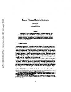
(These are the inverses of the transforms used in Equations 4 and 7.) They are plotted in Figure 1. We see that the two links are almost identical if the probability of an event is less than 25%, and are extremely similar so long as the probability of an event does not exceed 50%. If the probabilities of an event are not large it simply does not matter whether we use a logit or a cloglog link. And for typical event history data (especially in IR) the probability of an event in any given time period will be small. The two links will only differ in the unlikely case (for event history data) that many observations have a probability of failure exceeding 50%. And even here, who is to say whether the cloglog model is the right model? While the cloglog model is the exact grouped duration analogue of the Cox 20

To be concrete we show one particular assignment of the κ. t | 1 y | 0 κ | κ1

2 0 κ2

3 0 κ3

4 1 κ4

5 0 κ1

6 1 κ2

7 1 κ1

8 0 κ1

9 0 κ2

As with any saturated set of dummy variables we must either not estimate a constant term or drop one dummy variable. For notational simplicity we assume the former, though most statistical packages do the latter. This should cause no problems. 21 This terminology is from the “generalized linear model” (GLM) approach (McCullagh and Nelder 1989). A link function specifies the relationship between a linear predictor (x i,t β) and the dependent variable. The logit and cloglog links are two common links for binary dependent variable models.

8

Figure 1: Comparison of cloglog and logit transforms 15 logit cloglog 10

Transform

5

0

-5

-10

-15 0.0

0.2

0.4

0.6

0.8

1.0

Probability

proportional hazards model, and while the Cox proportional hazards is the most widely used model, is it is exactly the right model in all cases? The logit link corresponds to some (complicated) continuous time duration model (Sueyoshi 1995). While the Cox proportional hazards model is computationally convenient, there is no reason to assume that data is generated in a computationally convenient form. For typical BTSCS data there appears to be no cost to using the more familiar logit link. But there are clear benefits to using the logit link. It is well understood by researchers, is estimable with any software package, does not require learning new methods (generalized linear models) and, most importantly, is easier to extend in a variety of interesting ways.22 We therefore recommend that researchers use P (yi,t = 1|xi,t ) = h(t|xi,t ) =

1 1+

e−(xi,t β+κt−t0 )

(7)

which is the logistic analogue of Equation 4. 22

Allison (1982, 87-90) shows how the logit can be extended to the multinomial logit to handle multiple types of failures. Thus we could allow for data where yi,t denotes a series of unordered outcomes, so long as the outcomes satisfy the independent risks assumption underlying the “competing risks” model. Any remedies which allow logit to deal with cross-sectional dependence will also be easy to combine with the logit link.

9

Temporal dummy variables Using the logit rather than the cloglog link allows us to focus on the second way that Equation 7 differs from ordinary logit: the inclusion of the temporal dummies, κ t−t0 . These are the grouped duration analogue of the continuous time baseline hazard function, h0 . Omitting these dummies is equivalent to assuming that the baseline hazard is constant, so that the model shows duration independence. While such a situation can occur, event history analysts typically allow for duration dependence, at least initially, and then test for whether the model can be simplified by imposing duration independence. The costs of incorrectly imposing duration dependence are, at a minimum, inefficiency and incorrect standard errors, and may, in complicated cases, even lead to inconsistent parameter estimates. It is exactly these problems that the Cox proportional hazard model avoids.23 It is simple enough to include the temporal dummies in the logit specification. Before doing so one should test whether they are required. Temporal dummies should not be included in the specification if the observations are already temporally independent, since the temporal dummies might then introduce unnecessary multicollinearity. The test of whether the temporal dummies should be included is a standard likelihood ratio test of the hypothesis that all the κt−t0 = 0. If the null hypothesis of temporal independence is rejected then all the κt−t0 should be included in the logit specification. Thus Equation 7 is the generalization of ordinary logit that allows for temporally interdependent observations. It is, as we have just seen, easy to both test for, and correct the logit for, temporally dependent observations.

Cubic splines Equation 7 requires the estimation of the coefficients of many dummy variables. Unless N is large these will not be precisely estimated. While this is not a problem if our interest is in estimating β, we may have some interest in the κ themselves. Note that the κ t−t0 are easily interpretable as “baseline” probabilities (or hazards) in that P (yi,t = 1|xi,t = 0, t0) = κt−t0

(8)

While the path traced out by the κt−t0 is easily interpretable, the imprecision with which the κ are estimated may give a false impression that the baseline hazard is jagged. We would expect it to be smooth. One solution to this problem is to replace the dummy variables in Equation 7 with a smooth function of t − t0. (We cannot directly use t − t0 since there is no reason to assume that the baseline hazard is a linear function of time.) In earlier work we recommended “cubic smoothing splines” (Beck and Jackman 1997; Beck and Tucker 1996). But while these work very nicely, they do require software (such as 23

The Cox proportional hazard model differs from parametric duration models such as the Weibull in that the baseline hazard, h0 is not specified in the Cox formulation; parametric approaches require the researcher to fully specify h0 . Theory is often (perhaps usually) silent about the specification of h0 .

10

S-Plus) that is often not readily accessible. One can obtain almost the same degree of smoothness with “natural cubic splines” (Eubank 1988). The advantage of these is that they are easy to implement with widely available software packages (such as the spbase program available for Stata). Natural cubic splines fit cubic polynomials to a predetermined number of subintervals of a variable. These polynomials are joined at “knots,” with the number and placement of the knots specified by the analyst. Smoothness is imposed by forcing the splines, and their first and second derivatives, to agree at each of the knots. Thus each knot only uses up one degree of freedom, so that we can flexibly fit a cubic spline using up only a very few degrees of freedom. The estimated spline coefficients can then be used to trace out the path of duration dependence. One advantage of the spline is that it facilitates a test of the hypothesis of duration dependence. With many temporal dummy variables the likelihood ratio test for whether they are all zero may have poor finite sample properties. The equivalent test on the spline formulation only requires testing whether a small number of spline coefficients are zero. Analysts can freely choose either the dummy variable or the spline formulation. This choice has almost no consequences for the estimation of β. We have a slight preference for the spline formulation, but users hesitant to deal with natural splines can resort to the simpler dummy variable specification with little loss. We use both approaches in our replication, though we rely primarily on the spline approach. Since the logit with temporal dummy (or spline) variables is more general than ordinary logit, and since we can easily test the null hypothesis of duration independence, there is no reason not to undertake logit analysis of BTSCS data adding the temporal variables if they are required. This is not to say that there might not be better methods for estimating some models. While the Cox proportional hazards model is widely used and works well in practice, no model can be expected to be optimal for all problems. But we expect that logit analysis with temporal dummy or spline variables will work well for most BTSCS data sets. There can be no doubt that this approach is superior to ordinary logit.

3.3

Complications

Before turning to our re-analysis, there are several complications that we must discuss. These complications would not arise if the data were independent, but they are inherent if we are unwilling to make that assumption. The event history approach simply makes these problems (and possible solutions) clearer.

11

Multiple failures The first problem is that BTSCS data allows for multiple failures per unit. Many event history analyses simply model time until the first (or only) failure, but the nature of BTSCS data allows for more than one failure per unit.24 Ordinary logit avoids any problems by assuming that the probability of failure in any year is the same as in any other year (conditional only on the independent variables), so that second and subsequent failures are assumed to be generated identically to first failures. In our construction of the κ’s we have also used this assumption, since the only relevant information in the κ is time since the most recent event. However implausible the assumption that second and subsequent events are are independent of the number and timing of previous events, this assumption is weaker than the ordinary logit assumption that all observations are independent. Since the assumption that second spells are independent of first spells is questionable, one solution might be to limit the analysis to the initial event. While losing data on second events is inefficient, it does allow for consistent estimation of β without having to model the dependence of second and later events on earlier events. Of course it would be better to correctly model repeated events. One easy way to do this is to include in the specification a variable which counts the number of previous events. This approach, while primitive, is better than ignoring the problem. A related issue that is common in IR studies is that events may appear to take place over the course of several years. If conflicts really are multi-year we should simply drop all but the first year of the conflict from the analysis. If we have a theory about the duration of peace we should not include spells of conflict in testing that theory. But it also may be the case that we observe different conflicts in consecutive years, and so discarding the subsequent years of multi-year conflicts is really discarding new, but very short, spells of peace. A decision about what to do here can only be made on theoretical grounds. But if we observe multi-year spells of conflict it is hard to maintain the assumption that the yearly observations are independent of each other. Duration dependence may manifest itself in the finding that conflicts are more likely to follow other conflicts.

Left censoring The second problem has to do with what event history analysts call “left censoring.” Spells are left censored if we do not know when they began.25 For example, if our first dyadic observation is 1951, we do not know if a spell of peace began in 1951, 1950 or before. This may not be a large problem in IR, since we can often begin analyses at the start of a new international order or security regime (the Congress of Vienna or the 24

If only one failure per unit were possible, we should discard all data after the first failure. But in BTSCS data we have observations through a fixed time T . 25 Spells are “right censored” if we do not know when they ended. These are not a problem for grouped duration logit analysis. Units that are right censored simply contribute a string of zeros, with no final one, to the logit likelihood.

12

beginning of the Cold War). Our proposed method is also forgiving of left censoring so long as all observations are equally left censored. For example, if the Cold War started in 1947, but our data starts in 1954, left censoring causes literally no problems for our proposed method.26 All that is required is that the κ for any given year reflect the same length of prior peace spell length for all units. This could cause problems, for example, for dyads that enter the data set after the starting year. In our re-analysis, for example, some dyads enter the data set after one of the members became independent. Suppose the data set begins in 1951 but a dyad enters the data set in 1962. Should the dummy variable for that observation be κ1 or κ12 ? If our example (and in our re-analysis) it seems reasonable to use κ1 here. But analysts will have to make judgments before beginning their own data analysis. Result should be relatively insensitive to a few differences in judgment on this issue.

Variables that are fixed across units The third potential problem with our method is that it does not allow researchers to use independent variables that vary by time but not across units. In IR such variables are measured at the system level. Some examples of systemic level variables are the concentration of power or the number of nation-states in the world at any given time. These variables will be highly collinear with the κ.27 Inclusion of the κ in the specification makes it unlikely that the coefficients of these systemic variables will remain statistically significant. This will cause problems for some, but not all, research agendas. 28 Systemic level variables are, for example, rare in dyad-year studies of conflict. If system level variables account for most of the duration dependence, then our test for it will indicate that we cannot reject the hypothesis of duration independence. At that point researchers can confidently use ordinary logit analysis including system level variables. This is the optimal situation, since the system level variables theoretically explain duration dependence. We fear that this situation is rare. There may be other situations that remain problematic. If the system level variables are important we might choose to ignore duration dependence if it is not serious (as indicated by a baseline hazard function that looks fairly flat). Sometimes the cure may be worse than the disease! There will remain some situations where the researcher is simply faced with a choice between two evils. The analysis of data is an art, not a science. 26

All we lose are estimates of the nuisance yearly dummies from 1948 through 1953. See Jenkins (1995) for a formal proof and a good discussion of the interaction of grouped duration analysis with various sampling designs. Suppose the sample period begins with t2 but that spells actually began at t1 < t2. Jenkins shows that this is irrelevant for the estimation of β. 27 They are not perfectly collinear if there are multiple events per unit, since the κ then no longer simply mark t. They will also not be perfectly collinear with the temporal spline. But they might be highly collinear. 28 The problem is identical to that associated with fixed unit effects in models with independent variables that are constant within units. This problem has not caused researchers to abandon fixed effects modeling.

13

One simple method will never solve all possible problems. But a test for whether the temporal variables belong in the logit specification, even with the system level variables included, at least alerts the researcher to the existence of problems caused by temporally dependent observations.

Missing data The fourth problem is that missing data becomes more troublesome in the presence of duration dependence. The assumption of independence allows the analyst to omit all observations with missing data, subject, of course, to the usual caveats about missing data (Little and Rubin 1987). Our method also allows for the elimination of observations with missing data so long as the correct time dummy variable is still used. Thus we cannot allow missing observations on the dependent variable (or we must assume that we are missing no years of conflict). In practice we will encounter relatively little if any missing data in the conflict variable, since IR researchers have gone to great lengths to code this data. But missing data on the dependent variable could be a potential problem in other types of BTSCS analyses. Keeping these problems in mind, we now turn to a re-analysis of one prominent BTSCS study.

4

Reassessing the Liberal Peace

One of the most prominent propositions in the IR/IPE literature is that democracies do not wage war on each other. Levy (1988) has implied that this is the only law-like generalization in IR and has been confirmed in myriad empirical studies.29 Classical economic liberals have argued that economic interdependence also inhibits war. The idea that trading partners are less likely to engage in military conflict has also received extensive empirical support for almost two decades.30 Oneal et al. (1996) strengthened the confidence in these findings by showing that the effects of economic interdependence an democracy were inversely related to the onset of military hostilities, even when controlling for several important confounding factors. Oneal and Russett (1997) claim to have improved upon the Oneal et al. (1996) specification in an effort to further connect these two major strands of research on the causes of conflict. Oneal and Russett found that, during the Cold War era, trade, as well as democracy, inhibits militarized conflict. These results, seemingly the most robust of their genre, appear to have solidified the conventional wisdom regarding the relationships between economic interdependence, democracy, and war. They therefore conclude that the classical liberal prescription for peace, trade and democracy, is correct. 29

For a recent overviews of the democratic peace literature see Chan (1997) and Ray (1997). The first prominent statistical study was conducted by Polachek (1980) and the most recent analysis can be found in Gartzke (1998). For a recent overview of the economic interdependence literature see McMillan (1997). 30

14

Oneal and Russett (hereinafter O/R) performed ordinary logit analyses on BTSCS data without accounting for temporal dependence. We use our proposed method to re-analyze their data to see whether their findings survive more appropriate statistical tests. The dataset we use, provided by O/R, contains 20990 dyad-years, comprised of 827 “politically relevant dyads” observed annually from 1951 through 1985.31 Some dyads were observed for all 35 years, while others were observed for a shorter sub-period. The median observation length is 22 years.32 The dependent variable is DISPUTE, whether or not a dyad engaged in a militarized dispute in a given year. While earlier researchers typically used interstate war as a dependent variable, recent research has frequently examined militarized interstate disputes. Interstate wars are a small subset of militarized interstate disputes. The latter include any event involving the threat or actual use of military force while the former require a substantial number of battle deaths.33 The two key independent variables are democracy (DEM ), and economic interdependence (TRADE). Both of these are dyadic measures. DEM is constructed by creating democracy scores (using Polity III data) for each member of the dyad and taking the dyadic score as the lesser of the two (Oneal and Russett refer to this as the “weak link” assumption). We rescaled DEM to run from -1 to 1. TRADE measures the importance of dyadic trade to the less trade oriented of the two partners. The importance of trade is measured by the ratio (in percent) of dyadic trade to the GDP of each partner. Following O/R, TRADE is lagged one year so that low trade does not proxy a current dispute. O/R also use a series of control variables. ALLIES is a dummy variable measuring whether the dyad partners were allied (or both were allied with the United States). CONTIG is a dummy variable measuring whether both states are contiguous. CAPRATIO measures the dyadic balance of power. Using the Correlates of War material capabilities index, it is the ratio (in percent) of the stronger nation’s score to the weaker nation’s. Lastly, GROWTH measures the lesser of the rates of economic growth (as a percent) of the partners. Detailed discussion of the O/R data set and operationalizations is contained in their original paper. The analyses which correct for duration dependence either use a natural cubic spline in PEACEYRS or the set of dummy variables created from PEACEYRS. PEACEYRS counts the length of the spell of peace preceding the current observation. For observations with no previous dyadic disputes, PEACEYRS is simply t, the time index; subsequent to a dispute, PEACEYRS is t − t0 where t0 is the time index of the most recent recent dispute. PEACEYRS runs from zero to 34. 31

A dyad is “politically relevant” if the nations are geographically proximate or if one state is a major power. The analysis of politically relevant dyad-years is a prominent IR BTSCS design. 32 Their data set has gaps in some dyadic observations. We did not attempt to fill these in, but we did correct the temporal variables for these gaps. 33 We initially maintain O/R’s coding decision to count every dispute year as a separate dispute, even when many of these were merely a continuation of the same event. To get a bit ahead of ourselves, this decision turns out to have been crucial.

15

Column I of Table 1 shows the original O/R results. We were able to replicate Oneal and Russett’s original estimates exactly.34 We limit our re-analysis to the temporal dependence issues discussed in our paper. We also examine only their specification one and do not investigate alternative substantive models of conflict.35 These results show that both democracy and economic interdependence lower the probability of a militarized dispute; they appear to be both statistically and substantively significant. The control variables, as O/R predicted, also exhibit substantively important effects. A different picture emerges, however, once we correct for temporally dependent observations using grouped duration methods. Results are in Columns II and III for the logit link and Column IV for the cloglog link. A test for whether the temporal dummies are required (a likelihood ratio test of I vs II) or whether the temporal splines are required (I vs III) clearly show strong duration dependence; this can also be easily seen by looking at the t-ratios of the four terms that comprise the cubic spline in PEACEYRS: 14, 9, 7 and 4.36 Thus the O/R logits clearly show duration dependence. Estimation that accounts for duration dependence has dramatic consequences for the O/R finding. The effect of trade, in particular, is reduced by a factor of five (and becomes statistically insignificant). These results provide no evidence for a liberal economic peace. Not all coefficients are affected by controlling for duration dependence. Our re-analysis leaves the DEM coefficient and standard error almost unchanged. Thus while we find no support for the liberal economic peace, the liberal political peace hypothesis is upheld. 37 The consequence of controlling for duration dependence on any variable is difficult to predict in advance. But, as we see here, the consequences of failing to account for duration dependence in typical logit estimation are enormous.

4.1

Links and splines

We also observe that it makes no difference whether we use the logit or cloglog link. The estimates for the two different links are even more similar than Table 1 (Columns II and IV) indicates, since the transformation of the independent variables into probabilities differs slightly between the two links. The mean difference in predicted probabilities between the two models is .007% with only about 2% of all dyad-years having predicted 34

All of our analyses were done with Stata, Version 5. Note that some variables were rescaled to make for simpler tables. 35 Their other specifications are similar to the one we re-examine here. We have applied our method to their specifications two through six and obtained similar results. 36 Likelihood ratio tests of specification II versus I yielded χ2 statistics of 1778 with 31 degrees of freedom; the test of III versus I yields a statistic of 1789 with 4 degrees of freedom. The test of I versus II drops 916 perfectly predicted observations from both logits so that log likelihoods are comparable. The probability of obtaining either result by chance is, to computer precision, zero. Tests on specifications in subsequent tables reveal similar results and are not shown here. 37 The control variables are also differentially impacted. Although the effect of CAPRATIO is almost unchanged in magnitude and statistical significance, the effects of the three other control variables are cut by half (with GROWTH even becoming statistically insignificant).

16

Table 1: Comparison of ordinary logit and grouped duration analyses Ordinary Logit Variable DEM GROWTH ALLIES CONTIG CAPRATIO TRADE Constant

I −0.50 (0.07) −2.23 (0.85) −0.82 (0.08) 1.31 (0.08) −0.31 (0.04) −66.13 (13.44) −3.29 (0.08)

Logit Dummya II −0.55 (0.08) −1.15 (0.92) −0.47 (0.09) 0.70 (0.09) −0.30 (0.04) −12.67 (10.50) −0.94 (0.09)

PEACEYRS Spline(1)c Spline(2)c Spline(3)c

Grouped Duration Logit Cloglog Spline Dummyb III IV −0.54 −0.49 (0.08) (0.07) −1.15 −0.81 (0.92) (0.76) −0.47 −0.43 (0.09) (0.08) 0.69 0.55 (0.09) (0.08) −0.30 −0.30 (0.04) (0.04) −12.88 −12.50 (10.51) 9.96 −0.96 −1.11 (0.09) (0.08) −1.82 (0.11) −.24 (0.03) −.08 (0.01) −.01 (0.003)

Log Likelihood −3477.6 −2554.7 −2582.9 −2554.1 df 20983 20036 20979 20949 N=20990 Standard errors in parentheses a 31 temporal dummy variables in specification not shown 3 dummy variables and 916 observations dropped due to outcomes being perfectly predicted b 34 temporal dummy variables in specification not shown c Coefficients of of PEACEYRS cubic spline segments

17

probabilities of a dispute differing by more than 1%. Thus, as we recommend, subsequent analyses only use the logit link. Results using a natural cubic spline in PEACEYRS are in Column III. Comparing Columns II and III we see that it makes no difference in terms of estimating β whether we use temporal dummy variables or a cubic spline in PEACEYRS. Since we have a preference for the spline setup all subsequent analyses use the natural cubic spline in the length of prior spells of peace.38

4.2

Why duration dependence affects the findings on economic interdependence

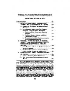
Accounting for temporal dependence clearly has dramatic effects on O/R’s finding that economic interdependence decreases conflict. Oneal and Russett (1997, 283) claim that they theoretically expect a high correlation between trade and length of spells of peace, and hence trade really does lessen conflict. But the problem in the O/R analysis is not with a correlation between trade and length of spells of peace, but a correlation between trade and lengths of spells of conflict, combined with a much higher than average probability of a conflict immediately following another conflict. Their proposed solution, to regress PEACEYRS on TRADE and then add the residuals from that regression to the logit specification, simply does not correct for temporal dependence. The temporal variables added to the logit specification to correct for duration dependence may not be arbitrarily changed without undoing the correction for temporally dependent observations.39 We can understand why accounting for duration dependence so strongly affects the O/R finding on trade by using some event history techniques. We begin with an examination of the estimated hazard function. This is computed for the logit analyses by setting all independent variables at their means (except for the two dummy variables which are 38

All splines allowed for three knots, placed at 1,4 and 7 years of peace. The number of knots was chosen by a sequence of F -tests; a variety of knot placements were tried with the chosen placement performing best. Results were insensitive to small changes in either the number or placement of the knots. The natural cubic spline estimated here is very similar to the smoothing splines shown in Beck and Jackman (1997) and Beck and Tucker (1996). We also reran the analyses for subsequent tables using temporal dummy variable and obtained almost identical results. Figure 2 also shows that it matters little if analysts add a cubic temporal spline or temporal dummy variables to the logit specification. 39 They also claim that a modified Cochrane-Orcutt correction for temporal dependence did not change their results. We know of no way to modify the Cochrane-Orcutt procedure to handle BTSCS data. Oneal and Russett (1997, 283) state that they “re-estimated [their] equation (6) with indicator variables for all years but one [with] results consistent with those [they] report.” We re-estimated their Equation 6 with temporal dummies and found that the coefficient on trade dropped by a factor of four (and became statistically insignificant), the coefficient on the trend of trade dropped by a factor of five (and also became statistically insignificant). While the coefficients on the two democracy variables declined by 30%, they remain strongly statistically significant. Finally O/R report that bootstrapped standard errors were only slightly different from their reported standard errors. Standard bootstrapping, however, does not work with interdependent observations (Freedman and Peters 1984).

18

set to their modal value of zero). The estimated hazard function, plotted against the length of peace spell, (PEACEYRS), is shown in Figure 2. Figure 2: Discrete hazard of dispute 0.25 Spline Dummies 0.20

Probability

0.15

0.10

0.05

0.0 0

5

10

15

20

25

30

35

Duration of Peace

The probability of a dispute immediately following a prior dispute is almost 25%. It immediately falls to about 5% the next year, and then falls to about 2% the third year, where it remains for the rest of the spell of peace. Thus, much of what the duration dependent logit highlights is the dependence of the probability of a dispute on an immediately preceeding dispute. Counting the latter years of multi-year disputes as new disputes, and failing to correct for dependence between these disputes, is what leads to their finding that trade lowers the probability of the onset of a dispute. It appears that economic interdependence does not dampen the probability of a dispute, but it does diminish the duration of a dispute once it occurs. Remember that TRADE is lagged one year so that the previous year’s trade predicts the current probability of a dispute. Trade averages 0.22% of GDP prior to one year disputes This is only slightly lower than the 0.23% of GDP that trade averages prior to a year of peace. But, in the last year of peace prior to a multi-year dispute, trade averages only 0.15% of GDP. Thus TRADE is not a good predictor of whether a dispute will occur, but it is a good predictor of whether, if a dispute occurs, it will be lengthy. Low trade may lengthen conflicts, but it does not appear to cause them.

19

4.3

The effect of multiple disputes

We can further examine the contaminating effects of long spells of disputes by dropping ongoing years of a dispute from the analysis. 542 dyad-years with a dispute are thus dropped.40 Results of this analysis are in Table 2. Table 2: Grouped Duration Analyses: No Continuing Dispute Years

Variable DEM GROWTH ALLIES CONTIG CAPRATIO TRADE Constant PEACEYRS Spline(1)a Spline(2)a Spline(3)a

I. Logit Ordinary βb se

−0.40 −3.43 −0.48 1.35 −0.20 −21.08 −4.33

0.10 1.25 0.11 0.12 0.05 11.30 0.11

II. Logit Group Dur. βb se

−0.39 −4.01 −0.37 0.99 −0.22 −3.81 −3.57 0.39 0.09 −0.03 0.003

0.10 1.25 0.11 0.12 0.05 9.68 0.17 0.16 0.03 0.01 0.003

Log Likelihood -1846.9 -1751.4 df 20441 20437 N=20448 a Coefficients of PEACEYRS cubic spline segments Dropping the latter years of a dispute, even without accounting for duration dependence, reduces the TRADE coefficient by a factor of three, leaving it barely statistically significant. A likelihood ratio test, however, clearly shows remaining duration dependence. When we account for this (Column II), the effect of dyadic trade is again greatly reduced and is now not even close to being statistically significant. Dropping ongoing dispute years, even accounting for duration dependence, has little effect on the democracy coefficient.41 We can also examine the contaminating effects of disputes on later disputes by confining our analysis to first disputes (eliminating observations on 3999 dyad years which followed an initial dispute). This analysis avoids any problems associated with the need to model the conditional probability of second and later disputes. Results are in Table 3, Column I. 40

All disputes that continue for more than one year are dropped, even if disputes in subsequent years have differing identification codes. 41 The estimated pacific impact of economic growth dramatically increases with the omission of ongoing dispute years.

20

Table 3: Grouped Duration Analyses: Second Disputes Differ

Variable DEM GROWTH ALLIES CONTIG CAPRATIO TRADE PRIOR DISPUTES (#) Constant PEACEYRS Spline(1)a Spline(2)a Spline(3)a

I. First Disputes βb se −0.46 0.13 −2.29 1.78 −0.42 0.16 1.11 0.17 −0.19 0.06 −3.55 11.73 −3.21 −1.08 −0.18 −0.07 −0.01

0.21 0.24 0.05 0.02 0.05

II. Prior Disputes βb se −0.41 0.08 −2.09 0.97 −0.25 0.09 0.69 0.09 −0.20 0.04 −9.39 10.19 0.17 0.01 −1.60 0.10 −1.67 0.11 −0.22 0.03 0.07 0.01 −0.01 0.003

Log Likelihood -964.1 -2393.0 df 16980 20978 N 16691 20990 a Coefficients of PEACEYRS cubic spline segments

Limiting our analyses to time until the first dispute eliminates about 20% of the data and results in an increase in all the standard errors. The pacific effect of democracy remains almost unaffected by this limitation (other than the increase in standard error). But once again there is a drastic decrease in the estimated impact of economic interdependence. Increased dyadic trade does not reduce the likelihood of a first dyadic dispute; democracy does. A less drastic way to allow for differing conditional probabilities of a dispute given the number of prior disputes is to add to the logit a counter measuring the number of prior dyadic disputes. These results are in Table 3, Column II. While the results are not as dramatic as the limitation to first disputes only, they clearly show the pacific effect of democracy but not of trade. Accounting for temporal dependence clearly has dramatic effects on O/R’s finding that trade decreases conflict. When the O/R estimation is corrected for that dependence the finding that trade reduces conflict simply disappears, although trade may reduce the length of conflicts once they occur. Our reassessment of the O/R finding, however, leaves intact their conclusion about the pacific effects of democracy.

21

5

Conclusion

The analysis of binary dependent variable time-series–cross-section data is becoming more common, particularly in the study of international conflict. Almost all analysis of this type of data has used ordinary logit, ignoring any issues arising from the temporal interdependence of the data. We have shown that that is easy to allow for temporal dependence in logit analysis if we realize that BTSCS data is grouped duration data. Such data can then be analyzed quite easily using a logit model but adding temporal dummy variables (or a temporal spline) to the specification. This can be done using any statistical software package. This remedy has advantages over other attempts to correct for temporal dependence in BTSCS data. Because it uses standard logit routines it is easy to combine our method with remedies for other problems. In particular, it is simple to combine our method with Huber (1967) standard errors, which solve other problems inherent in BTSCS data. It is also easy to allow for heterogeneity using our method (Jenkins 1995). One would not want to fix one problem such that it became extremely difficult to fix any other; real data is seldom subject to only one problem. A related advantage is that logit is well-known and well-understood by researchers. Our proposed method, however, does force analysts to think about some problems that naturally occur to the event history analyst (and which do not naturally occur to the logit analyst). In particular, our approach requires analysts to think about whether they are modeling spells of peace, spells of conflict, or both. It also requires consideration of modeling second and subsequent events for the same unit. These considerations are critical to the modeling process. There are clearly other possible ways to allow for temporal dependence in BTSCS data. Ideally we would model that dependence as a function of other variables. Our proposed method simply treats temporal dependence as a nuisance which impedes estimation of the β. Nothing is explained by noting that hazard rates change with time. Our treatment of duration dependence is similar to early methods for estimating time series models with serially correlated errors. While more modern treatments prefer the modeling of dynamics to thinking of serially correlated errors as an estimation nuisance, simply ignoring the nuisance can prove fatal. Current practice for BTSCS models is much like using OLS for correlated time series data. A theoretically based specification of this duration dependence would be best, but it is easier to give this advice than to implement it. In the meantime we surely do not wish to continue the current practice of ignoring potentially serious duration dependence. We have applied our methodological remedy to Oneal and Russett’s analysis of militarized conflict during the Cold War period. Oneal and Russett found that both political and economic liberalism inhibits conflict. Our re-analyses show that democracy clearly inhibits conflict, but trade does not. But while trade may not inhibit conflict, it does appear to shorten spells of conflict. The differences between the original analysis and 22

our re-analysis are considerable. Temporal dependence in BTSCS models is not a minor problem that can be ignored at the cost of a small error. And there is no reason to commit these errors. The inclusion of temporal variables in the specification is a simple solution, available to all researchers, providing a low cost cure to the problem of temporally dependent BTSCS data.

23

Appendix A The Simple Math of Grouped Durations This appendix derives the grouped duration model. We present it here for completeness and because many standard event history texts do not present this result. This appendix assumes familiarity with basic duration concepts. Start with a continuous time Cox proportional hazards model, so hi (t) = h0 (t)exi,t β

(9)

where i refers to units, t refers to continuous time, xi,t is a vector of independent variables and h0 (t) is the unspecified baseline hazard. Letting S(t) be the probability of surviving beyond t, we use the basic identity that Z t S(t) = exp(− h(τ )dτ ). (10) 0

We only observe whether or not an event occurred between time tk −1 and tk (assuming annual data) and are interested in the probability of this event, P (yi,tk = 1). This probability is one minus the probability of surviving beyond tk given survival up to tk − 1. Assuming no prior events (so t0 = 0) Using Equation 10, we then get Z tk hi (τ )dτ ) (11a) P (yi,tk = 1) = 1 − exp(− tk −1 Z tk exi,tk β h0 (τ )dτ ) (11b) = 1 − exp(− tk −1 Z tk xi,tk β h0 (τ )dτ ) (11c) = 1 − exp(−e tk −1

Since the baseline hazard is unspecified, we can just treat the integral of the baseline hazard as an unknown constant. Defining Z tk h0 (τ )dτ and (12) αtk = tk −1

κtk = log(αtk )

(13)

we then have P (yi,tk = 1) = 1 − exp(−exi,tk β αtk )

(14a)

xi,tk β+κtk

(14b)

= 1 − exp(−e

)

This is exactly a binary dependent variable model with a cloglog link. 24

References Allison, Paul D. 1982. “Discrete-Time Methods for the Analysis of Event Histories.” In Sociological Methodology, ed. Samuel Leinhardt. San Francisco: Jossey-Bass pp. 61– 98. Alt, James E., Gary King and Curtis Signorino. 1997. Estimating the Same Quantities from Different Levels of Data: Time Dependence and Aggregation in Event Process Models. Technical report. Department of Government, Harvard University. http: //Gking.Harvard.Edu/preprints.shtml. Barbieri, Katherine. 1996. “Economic Interdependence: A Path to Peace or a Source of Interstate Conflict?” Journal of Peace Research. 33(1):29–50. Beck, Nathaniel. N.d. “Modelling Space and Time: The Event History Approach.” In Research Strategies in Social Science, ed. Elinor Scarbrough and Eric Tanenbaum. Oxford University Press. Beck, Nathaniel and Jonathan N. Katz. 1995. “What To Do (and Not To Do) with Times-Series Cross-Section Data.” American Political Science Review. 89:634–47. Beck, Nathaniel and Jonathan N. Katz. 1997. “The Analysis of Binary Time-Series– Cross-Section Data and/or The Democratic Peace.” Paper presented at the Annual Meeting of the Political Methodology Group, Colombus, OH. Beck, Nathaniel and N. Katz, Jonathan. N.d. “Nuisance vs.Substance: Specifying and Estimating Time-Series–Cross-Section Models.” Political Analysis. Forthcoming. Beck, Nathaniel and Richard Tucker. 1996. “Conflict in Space and Time: Time-Series– Cross-Section Analysis with a Binary Dependent Variable.” Paper presented at the Annual Meeting of the American Political Science Association, San Francisco. Beck, Nathaniel and Simon Jackman. 1997. Getting the Mean Right is a Good Thing: Generalized Additive Models. Working paper. Political Methodology WWW Site. http://wizard.ucr.edu/polmeth/working_papers97. Bennett, D. Scott. 1996. “Security, Bargaining, and the End of Interstate Rivalry.” International Studies Quarterly. 40(2):157–84. Bennett, D. Scott. 1997. “Testing Alternative Models of Alliance Duration, 1816–1984.” American Journal of Political Science. 41(3). Box-Steffensmeier, Janet M. and Bradford S. Jones. 1997. “Time is of the Essence: Event History Models in Political Science.” American Journal of Political Science. 41(4). Bremer, Stuart A. 1992. “Dangerous Dyads: Conditions Affecting the Likelihood of Interstate War, 1816–1965.” Journal of Conflict Resolution. 36:309–41. Bueno de Mesquita, Bruce and David Lalman. 1992. War and Reason: Domestic and International Imperatives. First ed. New Haven: Yale University Press. 25

Chan, Steve. 1997. “In Search of Democratic Peace: Problems and Promise.” Mershon International Studies Review. 41(2):59–91. Cox, D. R. 1975. “Partial Likelihood.” Biometrika. 62:269–76. Diehl, Paul and Gary Goertz. 1993. “Enduring Rivalries: Theoretical Constructs and Empirical Patterns.” International Studies Quarterly. 37:147–71. Diggle, Peter J., Kung-Yee Liang and Scott L. Zeger. 1994. Analysis of Longitudinal Data. Oxford: Oxford University Press. Enterline, Andrew. 1996. “Driving While Democratizing.” International Security. 21:183– 196. Enterline, Andrew. 1997. “Fledgling Regimes: Is the Case of Inter-War Germany Generalizable?” International Interactions. 22(3):245–277. Eubank, Randall L. 1988. Spline smoothing and nonparametric regression. New York: Marcel Dekker. Farber, Henry S. and Joanne Gowa. 1997. “Common Interests or Common Polities: Reinterpreting the Democratic Peace.” Journal of Politics. 59(2):393–417. Freedman, David and Stephen Peters. 1984. “Bootstrapping a Regression Equation: Some Empirical Results.” Journal of the American Statistical Association. 79:97– 106. Gartzke, Erik. 1998. “Kant We All Just Get Along?: Opportunity, Willingness and the Origins of the Democratic Peace.” American Journal of Political Science. 42(1). Gleditsch, Nils Petter and H˚ avard Hegre. 1997. “Peace and Democracy: Three Levels of Analysis.” Journal of Conflict Resolution. 41(2):283–310. Hermann, Margaret G. and Charles W. Kegley. 1996. “Ballots, a Barrior against the Use of Bullets and Bombs: Democratization and Military Intervention.” Journal of Conflict Resolution. 40:436–460. Huber, Peter J. 1967. The Behavior of Maximum Likelihood Estimates Under NonStandard Conditions. In Proceedings of the Fifth Annual Berkeley Symposium on Mathematical Statistics and Probability, ed. Lucien M. LeCam and Jerzy Neyman. Vol. I Berkeley, Ca.: University of California Press pp. 221–33. Huth, Paul. 1996. Standing Your Ground: Territorial Disputes and International Conflict. Ann Arbor, Michigan: University of Michigan Press. Jenkins, Stephen P. 1995. “Easy Estimation Methods for Discrete-Time Duration Models.” Oxford Bulletin of Economics and Statistics. 57(1):129–38. Katz, Jonathan N. and Brian Sala. 1996. “Careerism, Committee Assignments and the Electoral Connection.” American Political Science Review. 90(1):21–33. 26

Lemke, Douglas and William Reed. 1996. “Regime Types and Status Quo Evaluations: Power Transition Theory and the Democratic Peace.” International Interactions. 22:143–164. Levy, Jack. 1988. “Domestic Politics and War.” Journal of Interdisciplinary History. 18:653–73. Little, Roderick J.A. and Donald B. Rubin. 1987. Statistical Analysis with Missing Data. New York: Wiley. Mansfield, Edward and Jack Snyder. 1996. “The Effects of Democratization on War.” International Security. 21:196–207. Mansfield, Edward and Jack Snyder. 1997. “A Response to Thompson and Tucker.” Journal of Conflict Resolution. 41:457–461. Maoz, Zeev. 1996. Domestic Sources of Global Change. Ann Arbor: University of Michigan. Maoz, Zeev. 1997. “Realist and Cultural Critiques of the Democratic Peace: A Theoretical and Empirical Re-Assessment.” International Interactions. 23:000–000. Maoz, Zeev and Bruce Russett. 1992. “Alliance, Contiguity, Wealth, and Political Stability: Is the Lack of Conflict Among Democracies A Statistical Artifact?” International Interactions. 17:245–267. Maoz, Zeev and Bruce Russett. 1993. “Normative and Structural Causes of Democratic Peace, 1946–1986.” American Political Science Review. 87(3):639–56. McCullagh, P. and J.A. Nelder. 1989. Generalized Linear Models. 2nd ed. London: Chapman and Hall. McMillan, Susan M. 1997. “Interdependence and Conflict.” Mershon International Studies Review. 41(2):33–58. Mousseau, Michael. 1997. “Democracy and Militarized Interstate Collaboration.” Journal of Peace Research. 34(1):73–87. Oneal, John R. and Bruce Russett. 1997. “The Classical Liberals Were Right: Democracy, Interdependence, and Conflict, 1950–1985.” International Studies Quarterly. 41(2):267–94. Oneal, John R., Francis H. Oneal, Zeev Maoz and Bruce Russett. 1996. “The Liberal Peace: Interdependence, Democracy and International Conflict.” Journal of Peace Research. 33(1):11–29. Poirier, Dale J. and Paul A. Ruud. 1988. “Probit with Dependent Observations.” Review of Economic Studies. 55:593–614. Polachek, Solomon. 1980. “Conflict and Trade.” Journal of Conflict Resolution. 24:55–78. 27

Prentice, R. and L. Gloeckler. 1978. “Regression Analysis of Grouped Survival Data with Application to Breast Cancer Data’.” Biometrics. 34:57–67. Raknerud, Arvid and H˚ avard Hegre. 1997. “The Hazard Of War: Reassessing Evidence of the Democratic Peace.” Journal of Peace Reseach. 34(4). Ray, James Lee. 1997. “The Democratic Path to Peace.” Journal of Democracy. 8(2):49– 64. Russett, Bruce. 1990. “Economic Decline, Electoral Pressure, and the Initiation of International Conflict.” In The Prisoners of War, ed. Charles Gochman and Ned Allan Sabrosky. Lexington, MA: Lexington Books pp. 123–140. Russett, Bruce. 1994. Grasping the Democratic Peace. Princeton, New Jersey: Princeton University Press. Sueyoshi, Glenn T. 1995. “A Class of Binary Response Models for Grouped Duration Data.” Journal of Applied Econometrics. 10(4):411–31. Vasquez, John A. 1993. The War Puzzle. First ed. Cambridge: Cambridge University Press.

28