Beyond the Standard Model: Proton Properties S. Reucroft1 and E. G. H. Williams2 ThinkIncubate, Inc., Wellesley, Mass., USA July, 2015 Abstract: We present a simple, semi-‐classical e-‐model of the proton that gives the proton mass, charge, spin and magnetic moment that are all in good agreement with measurements. Introduction It was demonstrated several decades ago [1] that the proton is a composite object containing point-‐like fundamental particles. It is now usually assumed that there are three of these point-‐like objects (known as quarks) and that two of them have charge 2/3e, where e is the electron charge, and the other has charge -‐1/3e. They are somehow confined in a soup of virtual quarks and gluons. These assumptions are subject to interpretation and they have not been verified experimentally. In particular, neither quarks, gluons nor fractional charge have ever been detected directly in an experiment. In fact, the electron and positron are the only massive, charged point-‐like particles that are known to exist, so in this paper we assume that the proton is composed of two positrons and one electron. We choose three components because that is the simplest possible assumption. Of course this assumption is also subject to interpretation and it has also not yet been verified experimentally, but it has some features that are more palatable than the quark model and it does lead to some natural consequences and predictions that we present in this paper. Our assumption, then, is that the proton is composed of two positrons and one electron in an orbital structure not unlike that of a simple atom. The two positrons have relativistic orbital velocities and the electron is at rest. We refer to this model as the e-‐model. In an earlier paper [2] we introduced a model of the electron that interprets the electron (and positron) as a point-‐like object whose mass and charge are related by a simple self-‐mass formula that includes both gravitational and electrostatic self-‐ energy. Given the electron charge, in order to derive the experimentally determined electron mass we have to assume that, inside the electron, the gravitation parameter is some forty orders of magnitude larger than the well-‐known macroscopic value of 1
[email protected]
2
[email protected]
1
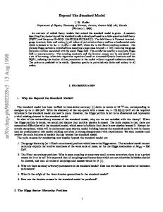
G [3]. The e-‐model of the proton also necessitates a very large value of G inside the proton. In the following, we refer to this short distance value of G as G0. In the earlier paper we made the assumption that the two positrons are in the same orbit with radius R = R1 and the electron is at rest at R = 0. The model used the measured values of proton and electron masses to obtain R1 = 0.8417 fm [2]. This is a simple and attractive model but it is not supported by the experimentally determined proton charge structure shown in figure 1 (solid curve). Therefore, in this paper we consider a slightly more complicated version of the model in which the two positrons are in separate orbits with R = R1 and R = R2, respectively, and the electron is at rest at R = R0 = 0. We assume that Coulomb repulsion causes the two positrons to be on opposite sides of the electron. Charge In the conventional quark model of the proton we have to face the uncomfortable fact that the proton charge appears to be exactly equal in magnitude to the electron charge. Since electrons and quarks are unrelated particles there is no explanation of how or why the quark charges should be exactly 2/3e and -‐1/3e. In our model the proton charge is, by definition, exactly the same magnitude as the electron charge so long as electron and positron have exactly equal and opposite charge, as is supported experimentally [3]. The distribution of charge inside the proton has been obtained from its electric and magnetic form factors [4, 5]. A recent particle physics planning report gives the current status based on a compilation of all available data [6]. As seen in figure 1 (solid curve), the charge is zero at the proton centre (R = 0), rises to a maximum at ~ 0.45 fm (1 fm = 10-‐15 m) and falls slowly to zero by ~ 2.5 fm. More than 90% of the proton charge is within a radius of 1.5 fm. The experimental uncertainty at the peak is ~ 4%. We have tested our model by attempting to fit the measured proton charge distribution of figure 1 to the sum of 3 electron charge distributions (2 positive and 1 negative). Initially we used Gaussian line shapes for the electron distributions. The fit was reasonable below about 1 fm, but the experimental charge tail above ~ 1 fm is too large to be consistent with a sum of Gaussians. We next tried Breit-‐Wigner line shapes3 and obtained an excellent description of the total proton charge distribution. The dashed curve in figure 1 shows the resulting 3 BW
€
(R) =
(Γ/2) 2 where R0 is the central value and Γ the width. (R − R0 ) 2 + (Γ/2) 2
€
2
sum of the 3 Breit-‐Wigners with best fit parameters: R0 = 0 and Γ0 = 1.20 ± 0.05 fm; R1 = 0.35 ± 0.02 fm and Γ1 = 0.97 ± 0.05 fm; R2 = 0.47 ± 0.02 fm and Γ2 = 0.93 ± 0.05 fm. We did not constrain the charge to be zero at R = 0 in any fit. €
€
€
€
€
Figure 1: Proton Radial Charge Distribution
140
Charge (arb. units)
€
€
€
120 100 80 DATA
60
BW SUM
40 20 0 -20
0
0.5
1
1.5
Radius, R (fm)
2
2.5
3
This supports the basic idea that the proton is composed of two positrons plus one electron. For calculation purposes, we assume that both positrons are at well-‐ defined orbital radii (R1 and R2, respectively) and the electron is at rest at R0 = 0. The reality is certainly more complex. It is not clear what is the significance, if any, of the Breit-‐Wigner line shape. Spin None of the components of the proton have orbital angular momentum (see the section entitled “Mass and Gravity”), so the spin of the proton is obtained by adding together the three spins. It is probably forbidden by something like the Pauli Exclusion Principle to have both positrons and the electron all with the same spin orientation inside such a small system, therefore we assume that the two positron spins cancel (one spin up, one spin down). The spin of the proton is then, by definition, exactly equal to the spin of the electron.
3
Magnetic Moment In the e-‐model, the magnetic moment of the proton ( µ p ) may be written as the sum of two terms. These are the current loop of the two orbital positrons and the mass-‐ scaled magnetic moment ( µe ) of the central electron:
µ p = µe
m€ e + IA , mp
€ where I is the current and A is the area of the loop.
The current loop term for € each orbital positron (radius R and velocity v) may be written: IA =
eπR 2v . 2πR
So, the expression for the proton magnetic moment becomes: € µ = µ me + 1 e(v R + v R ) . p e mp 2 1 1 2 2
With R1 = R2 = 0.4 fm and v1 = v2 = c, µ p = 14.16 x 10-‐27 J/T = 2.8 nuclear magnetons; this is in good agreement with the measured value of 2.793 nuclear magnetons [3]. € € Mass and Gravity We assume that the two positrons are in separate orbits with R = R1 and R = R2, respectively, and the electron is at rest at R = R0 = 0. We assume that Coulomb repulsion causes the two positrons to be on opposite sides of the electron. The quantum conditions for the two positrons are:
γ1me v1R1 = γ 2 me v 2 R2 = 2 c 2 ) and is the reduced Planck where γ1,2 are the relativistic factors (1/ 1 − v1,2 constant (h/2π). Note € that these quantum conditions have nothing to do with angular momentum. In a semi-‐classical sense, they are saying that the positron de Broglie wavelength ( λ = h p = h γmv ) has to equal € the circumference of the orbit. € €
If the total internal vector momentum is zero, the effective mass of the two positrons plus one electron is: € 1 1 m p = me (1+ γ1 + γ 2 ) = me + ( + ) . v1R1 v 2 R2
€
4
The kinematic limit gives R1 + R2 = 0.8417 fm with R1 = R2. These values of R1 and R2 give a good description of the proton charge distribution, they give a good approximation to the measured proton magnetic moment and they give the measured proton mass exactly, assuming the measured electron mass. € For every value of R1 + R2 above 0.8417 fm, there is one solution for the positron radii that gives the measured proton mass exactly. For all of these solutions, R1 ≠ R2 . In fact, given the Coulomb repulsion between the two positrons one of these solutions with the two radii not quite equal might be preferred. (For example, R1 = € 0.373 fm and R2 = 0.483 fm gives the measured proton mass.) € Since γ1 and γ 2 are both ~ 1000, the approximation v1 = v 2 = c is good to better than 1 part in 106. Therefore the formula for m p may be written: €
1 1 m p = me + €( € + ) . c R1 R2 € The equation of motion of either positron may be used to estimate the gravitation parameter G0. For example, for the outer positron (ignoring small terms): € γ 2 me v 22 G0γ1γ 2 me2 = . R2 (R1 + R2 ) 2 €
And this gives: 2 2 2 2 € G = v 2 (R1 + R2 ) = (R1 + R2 ) . 0 γ1R2 me γ1γ 22 R23 me3
€
At the kinematic limit R1 = R2 = R, γ1 = γ 2 = γ , v1 = v 2 = v and G0 = 4 2 γ 3 me3 R = 4v 2 R γme = 1.8 x 1029 Nm2/kg2. € For all values of R1 and R2 consistent with the proton charge distribution and the € 2 < 0.85 fm, say) the value of G € € proton magnetic moment (R1 + R 0 is in the range 1.4 29 2 2 to 2.4 x 10 Nm /kg . Finally we note that in this model the proton self-‐mass is given by:
SM = me +
G0γ1me2 G0γ 2 me2 G0γ1γ 2 me2 v1 v 2 + + . 2 2 2 = me + 2 + R1c R2c (R1 + R2 )c R1c R2c 2
It is perhaps worthy of note that when v1 = v2 = c, this is exactly equal to the effective mass of the two positrons plus one electron. €
5
Schwarzschild Radius The Schwarzschild radius of an object of mass m is given by: RS =
2Gm , c2
where G is the gravitation parameter and c the speed of light in vacuo. For the value of G0 given here € for the interior of the proton4, the value of RS = 6.7 fm. For the electron model described in [2] the value of G0 inside the electron could be as high as 2.8 x 1032 Nm2/kg2 in which case RS = 5.6 fm. In both cases the Schwarzschild radius is significantly greater than the physical radius. Could this be a hint as to why both proton and electron are very stable? Antimatter and Matter In the Standard Model of particle physics there is a problem because there appears to be significantly more matter than antimatter in our universe. This is not a problem with the e-‐model discussed in this paper. In a charge-‐neutral universe there are an equal number of electrons and positrons. If the electron is matter, then the positron is antimatter and vice versa. The fundamental matter-‐antimatter balance is between positive and negative electrons. All other particles are composite objects containing some matter and some antimatter. The neutron and all atoms contain an equal quantity of matter and antimatter. By definition, there is no matter-‐antimatter asymmetry. Conclusions and Predictions In this paper we introduce the e-‐model of the proton that takes us beyond the Standard Model. The proton is assumed to be composed of an electron and two positrons that are completely contained in a sphere of radius ~ 2.5 fm. They are assumed to be at radii of zero, R1 and R2, respectively and are held together by gravitational forces with a gravitation parameter G0 that is approximately forty orders of magnitude larger than the macroscopic value. All of the measured proton properties are consistent with the calculated quantities provided by this model. There is no acceptable quantum theory that governs this situation and so our calculations are made within a simple, semi-‐classical framework. 4 We are making the assumption that G is dominated by its short distance value G . 0
The same is true of the formula for self-‐mass in the previous section.
6
It is remarkable that such a simple model can calculate the exact proton mass and magnetic moment, charge and spin that are all in excellent agreement with measured values. However, it is interesting that the charge distribution and the magnetic moment both prefer R1 + R2 ~ 0.8 fm whereas the proton mass calculation requires R1 + R2 ≥ 0.8417 fm, where R1 and R2 are the positron orbital radii. This might be a clue or it might be simply reflecting the approximate nature of the model. € Indeed, we are not suggesting that this is an exact description of the proton. It is, at € € best, a good approximation that might lead us in the right direction. The results of the calculations indicate that we might be on the right track.
Two other interesting features of the e-‐model are a natural matter-‐antimatter symmetry in the universe and a hint of a rationale for the stability of the electron and the proton. If the model does have some validity, then we can make some predictions that ought to be testable in well-‐designed experiments. These have been discussed elsewhere [2]. Two of them are worth repeating here: -‐ -‐
The gravitation parameter has to drop from ~ 1029 Nm2/kg2 to ~ 10-‐11 Nm2/kg2 as distances increase from ~ 10-‐15 m to ~ 10-‐2 m. This should be detectable; It should be possible to produce single protons and single antiprotons in e +e − collisions via the reactions e +e − → pe − and e +e − → pe + . An e +e − experiment below the pp threshold (at 1.85 GeV, say) ought to produce detectable ~ 700 MeV/c protons and antiprotons. € € € €
€ Acknowledgements
We thank Paolo Palazzi for reminding us of the classic papers on proton structure [4, 5] and for pointing out that our earlier version of the e-‐model was not supported by their results. We also thank Chris Johnson for useful comments and for running a cross-‐check of the proton charge distribution fits.
7
References [1] For an excellent review, see M. Riordan, SLAC-‐PUB-‐5724 (1992). See also J. I. Friedman and H. W. Kendall, Ann. Rev. Nucl. Sci. 22, 203 (1972) and the published versions of the Nobel lectures: R. E. Taylor, Rev. Mod. Phys. 63, 573 (1991); H. W. Kendall, Rev. Mod. Phys. 63, 597 (1991); J. I. Friedman, Rev. Mod. Phys. 63, 615 (1991). [2] S. Reucroft and E. G. H. Williams, “Proton and Electron Mass Determinations”, viXra 1505.0012 (2015). http://viXra.org/abs/1505.0012. This paper was originally posted on the arXiv, but it was deemed “inappropriate” by the arXiv moderators and removed. Even after a very lengthy appeal process, no explanation was ever given. [3] K. A. Olive et al., “Review of Particle Physics”, Chi. Phys. C. 38 (2014). [4] R. M. Littauer, H. F. Schopper and R. R. Wilson, Phys. Rev. Letters 7, 141 (1961). [5] R. M. Littauer, H. F. Schopper and R. R. Wilson, Phys. Rev. Letters 7, 144 (1961). [6] See page 26 in “The Frontiers of Nuclear Science, A Long Range Plan”, DOE/NSF Nuclear Science Advisory Committee (2008) and arXiv:0809.3137 (2008).
8