arXiv:hep-th/9910005v3 10 Feb 2000. NUP-A-99-16 hep-th/9910005. Bi-Local Higgs-Like Fields Based on. Non-Commutative Geometry. Shigefumi Naka, Shinji ...
NUP-A-99-16 hep-th/9910005
Bi-Local Higgs-Like Fields Based on
arXiv:hep-th/9910005v3 10 Feb 2000
Non-Commutative Geometry Shigefumi Naka, Shinji Abe,* Eizou Umezawa and Tetsu Matsufuji Department of Physics, College of Science and Technology Nihon University, Tokyo 101-8308, Japan *Ibaraki Prefectural University of Health Sciences, Ibaraki 300-0394, Japan
Abstract The bi-local model of hadrons is studied from the viewpoint of non-commutative geometry formulated so that Higgs-like scalar fields play the role of a bridge, the bilocal fields, connecting different spacetime points. We show that the resultant action for Higgs-like scalar fields has a structure similar to that of the linear sigma model. According to this formalism, we can deduce the dual nature of meson fields as the Nambu-Goldstone bosons associated with chiral symmetry breaking and bound states of quarks.
1
typeset using P T P TEX.sty
§1. Introduction In the resent understanding, the meson fields are believed to be bound states of quarks (q) and anti-quarks (¯ q ) represented by gauge invariant states such as hq¯2 Φ(C)q1 i0 in the H µ
sense of QCD; here, Φ(C) = P ei C Aµ dx and P is the path-ordering along the path C that connects q¯2 and q1 . 1) The QCD approach, however, requires non-perturbative calculations to analyze the bound states, and at the moment, only numerical approaches based on lattice gauge theory are available to study those states. The bi-local field proposed originally by Yukawa 2) has been studied by many authors in the context of relativistic two-body models of quark and anti-quark bound states. 3) The standpoint of those approaches is rather simple: In general, Φ(C) is a complicated functional of the path C; when C is a straight line, however, the field hq¯2 Φ(C)q1 i0 becomes a bi-local field B(x, y) expected to satisfy 1 2 (∂ + ∂y2 ) + V (x − y) B(x, y) = 0, (1) 2 x where V (x) is an effective potential representing the interaction between q and q¯. In such �
�
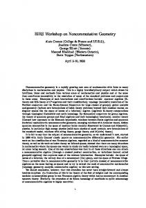
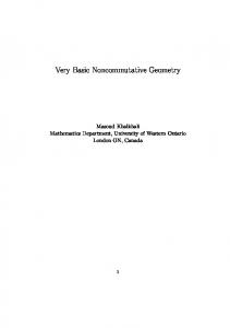
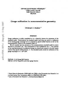
a model, we can calculate various phenomenological features of hadrons. In particular, the covariant oscillator quark model (COQM) that uses V (x) ∝ x2 is known to yield fairly good results. 4) From another point of view, however, the ground states of mesons, the pions, are usually understood as Numbu-Goldstone (N.G.) bosons associated with the chiral symmetry breaking of quark dynamics. It is not obvious that the two interpretations, bound states and N.G. bosons, for pions are compatible. Recently, a possible way of regarding the Higgs field as a gauge field was proposed by Connes and Lott 5) from the viewpoint of non-commutative geometry (NCG) and developed by many authors. 6) In their theory, spacetime is regarded as a product of the usual 4dimensional spacetime and a discrete two-point space. In those theories, the Higgs fields, which cause the gauge symmetry breaking, play the role of a bridge connecting two kinds of matter fields, the Dirac fields Ψ¯R (x) and ΨL (x), at the same spacetime point x (Fig. 1). Then, as an extension of this type of symmetry breaking, it may be possible to introduce Higgs-like fields Φ(x, y) which connect two kinds of matter fields defined at different spacetime points x and y, say Ψ¯R (x) and ΨL (y). From our point of view, the two sheets picture in Fig. 2 describe the proper understanding, and ΨL and ΨR are treated as fields in one spacetime. In such a case, we may formulate the bi-local field in Eq. (1), the bound states of q¯ and q fields, as Higgs-like fields, which are related with the chiral symmetry breaking at different spacetime points x and y (Fig. 2). The purpose of this paper is, thus, to study the relationship between the picture of the bound-state and that of the Nambu-Goldstone field 2
5
[5
5
[ Φ �[
/
Φ� [ / � [ 5
/
[
Fig. 1. Higgs NCG.
fields
in
local
[/
Fig. 2. Higgs-like fields in bilocal NCG.
for some bi-local fields from the point of view of an extended NCG method.
∗)
The basic formulation is presented in the next section within the framework of a U(1/1) toy model. An attempt to extend this toy model to a more realistic QCD-type model is studied in §3. Section 4 is devoted to summary and discussion.
§2. Formulation of bi-local Higgs-like fields The original Connes-Lott formulation for the gauge theory based on NCG is not always convenient for our purposes. In what follows, we use the matrix formulation for such a theory developed by Coquereaux et al. 8) To construct the local U(1/1) gauge and Higgs field theories according to the ! matrix 0 1 1 ηˆ, where ηˆ = , as a formulation, first, we introduce the off-diagonal matrix η = 2M 1 0 kind of coordinate variable of the Dirac field Ψ (x) = (ΨL (x), ΨR (x))T . Here, M is a parameter with the dimension of mass and the off-diagonal elements ”1” in ηˆ represent unit matrices in ΨL /ΨR space. Second, with analogy to the equation ∂x f (x) = i[ˆ p, f (x)] for ordinary variables, we define the derivative of a 2 × 2 matrix A with respect to η by ∂η A = i[π, A} ≡ i([π, Ae ] + {π, Ao }),
(2)
where Ae and Ao are the block-diagonal and off-block-diagonal parts of A, respectively, and π is the momentum operator conjugate to η defined by {π, η} = −1 in the sense of quantum mechanics. An explicit form of π is given by π = −M ηˆ. Then, one can easily verify the normalization conditions (∂η )2 A = 0,
∂η η = −i, ∗)
An early attempt following this line is given in Ref. 7).
3
(3)
in addition to the Leibniz rule
∗)
˜ η B), ∂η (AB) = (∂η A)B + A(∂ ˜ η Ψ ), ∂η (AΨ ) = (∂η A)Ψ + A(∂
(4) (5)
where A˜ = Ae − Ao . In terms of the matrix iπ, one can also define the operation of ∂η on matter fields by ∂η Ψ = iπΨ . Now, we can define the covariant derivative operators under the local gauge and discrete transformations. As the generators of U(1/1) , we take the following: L
T =
1 0 0 0
!
,
R
T =
0 0 0 1
!
,
Q=
0 1 0 0
!
,
†
Q =
0 0 1 0
!
.
(6)
Then, in the extended spacetime (xµ , η), one can define the covariant derivatives acting on matrix and matter fields Ψ by Dµ Dη ˜η D
DµL 0 = ∂µ − + = , 0 DµR ! 0 φ † ∗ = ∂η − ig(φQ + Q φ ) = ∂η − ig , φ∗ 0 ! 0 Φ † ∗ = iπ − ig(φQ + Q φ ) = −ig , Φ∗ 0 ig(WµL T L
WµR T R )
!
(7) (8) (9)
where DµL/R = ∂µ − igWµL/R and Φ = φ + Mg . The last of them one is a covariant derivative operator with respect to η acting on matter fields. It should be noted that [Dµ , Dη ] = ˜ η ] and D 2 = D ˜ 2 − (iπ)2 , where the term (iπ)2 is one origin of symmetry breaking. [Dµ , D η η In terms of these matrices, the Lagrangian density for the U(1/1) gauge theory is given by † 1 † TrFAB F AB (FAB = gi [DA , DB }, A, B = µ, η). Here Fµν F µν and Fµη F µη are kinetic terms 4 † for gauge and scalar fields, respectively. Furthermore, Fηη F ηη gives rise to the potential term for the scalar fields. In addition, the Yukawa coupling between the matter fields and the ˜ ηΨ . scalar field is also given by Ψ¯ iD
Now let us attempt to extend the above gauge-Higgs system to one consisting of local gauge fields bi-local Higgs-like fields. The matter fields in this case should be written " Land # Ψ (xL ) as Ψ = , where xLµ and xR µ are independent coordinate variables. Accordingly, Ψ R (xR ) the indices L and R designate spacetime points in addition to gauge or chiral components in the extended formalism. As for the discrete variables η and π, we try the same form as in the local NCG, but M may be a c-number function of (xL − xR )2 if we consider The nilpotency ∂η2 = 0 is satisfied by ∂η A = α[π, Ae ] + β{π, Ao } for any α, β. However, the Leibniz rule (4) holds only for α = β. ∗)
4
translational invariance. Then, writing ∂µL/R = ∂/∂xL/R,µ , one can define the following as covariant-derivative operators acting on extended matrix or matter fields: DµL±
DµL ± ∂µR 0 0 0
=
DµR± =
0 0
!
= (DµL ± ∂µR )T L ,
(10)
!
= (DµR ± ∂µL )T R , 0 DµR ± ∂µL ! 0 φLR Dη = ∂η − ig , φRL 0 ! ! 0 Φ M LR ˜ η = −ig D , ΦLR = φLR + , g ΦRL 0
(11) (12) (13)
where DµL/R = ∂µL/R − igWµL/R (xL/R ), ΦLR = Φ(xL , xR ), and ΦRL = Φ† (xR , xL ). Indeed, since the gauge transformations Ψ → UΨ are induced by U=
"
U L (xL )
0
0
U R (xR )
#
(U L† U L = U R† U R = 1),
,
(14) ′
the operators in (10) - (13) undergo the transformations UDµL/R± U † = DµL/R± , UDη U † = Dη′ , and so on. Here, the primes indicate covariant-derivative operators, in which the gauge and scalar fields are replaced, respectively, by ′
WµL/R → WµL/R = U L/R WµL/R U L/R† +
i L/R L/R L/R† U ∂µ U , g
′
ΦLR → ΦLR = U L ΦLR U R† .
(15) (16)
In this sense, (10) - (13) define covariant-derivative operators provided (15) and (16) hold. It should be noted, however, that ΦLR obeys the bi-linear transformation (16). Then, φLR does not obey simple bi-liniear transformations under gauge transformations, due to the factor M, and vice versa. For the time-being in this section, we assume the transformation (16). For later purposes, let us introduce the center of mass variables Xµ = 12 (xLµ + xR µ ) and the relative variables x¯µ = xLµ − xR µ , in terms of which we can write 1 1 xLµ = Xµ + x¯µ , xR ¯µ , µ = Xµ − x 2 2 � � ∂ L R ¯µ = ∂ = 1 ∂ L − ∂ R . = ∂ + ∂ , ∂ ∂µ = µ µ µ ∂X µ ∂ x¯µ 2 µ
(17) (18)
It is, thus, obvious that by taking the limit xLµ , xR µ → xµ , the extended derivative operators DµL/R+ and Dη will tend to the local operators (∂µ − igW L/R )T L/R and Dη , respectively. On the other hand, DµL/R− will tend to −igWµL/R T L/R . 5
The candidates for the field strength constructed out of these extended covariant-derivative operators are L [DµL± , DνL± ] = [DµL∓ , DνL± ] = −ig∂[µ Wν]L T L = −igFµν ,
(19)
R [DµR± , DνR± ] = [DµR∓ , DνR± ] = −ig∂[µ Wν]R T R = −igFµν ,
(20)
{Dη , Dη } = −2g 2 ΦLR ΦRL −
!
1 2 M = −igFηη . g2
(21)
In contrast to the case of local covariant-derivative operators, however, [DµL+ , Dη ], etc., remain as operators in the following sense: i
h
[DµL+ , Dη ] = −ig (∂µ − igWµL )ΦLR Q − ΦRL (∂µ − igWµL )Q† ,
(22)
[DµL− , Dη ] = −ig (2∂¯µ − igWµL )ΦLR Q − ΦRL (2∂¯µ − igWµL )Q† , h
i
(23)
i
h
[DµR+ , Dη ] = −ig −ΦLR (∂µ − igWµR )Q + (∂µ − igWµR )ΦRL Q† ,
(24)
[DµR− , Dη ] = −ig ΦLR (2∂¯µ + igWµR)Q − (2∂¯µ + igWµR )ΦRL Q† .
(25)
i
h
In order to obtain the c-number field strength, we have to take the combinations such that [DµL+ + DµR+ , Dη ] = −ig n
hn
o
(∂µ ΦLR ) − ig(WµL ΦLR − ΦLR WµR ) Q o
+ (∂µ ΦRL ) − ig(WµR ΦRL − ΦRL WµL ) Q† + = −igFµη ,
[DµL− − DµR− , Dη ] = −ig
i
o
+ 2(∂¯µ ΦRL ) + ig(WµR ΦRL + ΦRL WµL ) Q† n
(26)
2(∂¯µ ΦLR ) − ig(WµL ΦLR + ΦLR WµR ) Q
hn
o
− = −igFµη .
i
(27)
L R ± Here, Fµν and Fµν are local field strengths, while Fηη and Fµη are bi-local field strengths. Therefore, in this model,
SGH
� 1 Z 4 � L Lµν R = − tr d x Fµν F + Fµν F Rµν 4 Z � � Z 1 1 † + † +µη − † −µη 4 R 4 L − tr d x + (Fµη ) F + Fηη Fηη d x (Fµη ) F 2 2
(28)
is a natural form of the action defined from these field strengths. This form preserves the L ↔ R invariance and tends to the action for the local gauge and Higgs fields in the limit xL → xR . The interaction between the matter fields and gauge-Higgs fields should also be given by SM =
Z
d4 xL
Z
˜ η Ψ, d4 xR Ψ δ (4) (xL − xR )iγ µ Dµ + iκD n
o
6
(29)
where κ is a parameter. Then in terms of component fields, the action S = SGH + SM can be written as 1 S=− 4Z
Z
+
d4 xL
−2g
2
+
Z
�
L R µνR F µνL + Fµν F d4 x Fµν
Z
Z
�
Z
1 ΦLR ΦRL − 2 M 2 g
4 R
dx
n
�
!2
d4 xΨ iγ µ ∂µ − ig WµL T L + WµR T R
+gκ
Z
d4 xL
2 �
¯ µ ΦLR d4 xR |Dµ ΦLR |2 + 4 D
4 L
dx
�
Z
�
L
R
�o
Ψ �
d4 xR Ψ ΦLR Ψ R + Ψ ΦRL Ψ L ,
(30)
where Dµ ΦLR = ∂µ ΦLR − ig(WµL ΦLR − ΦLR WµR ), ¯ µ ΦLR = ∂¯µ ΦLR − 1 ig(W L ΦLR + ΦLR W R ), D µ µ 2
(31) (32)
and the contractions Dµ ΦLR D µ ΦRL , etc., have been abbreviated as |Dµ ΦLR |2 , and so on. In the above action, the potential for ΦLR has a minimum at ΦLR ΦRL = g12 M 2 . There are several ways to choose the vacuum, and the following may coincide in the local limit xL → xR : 1 i) ΦLR = M + UL Φ˜LR UR† , g 1 ii) ΦLR = UL ( M + Φ˜LR )UR† . g
(33) (34)
Here, U L and U R are unitary-matrix fields that transform as U L/R → U L/R U L/R under the gauge transformation. Φ˜LR is assumed to be a gauge-invariant field. The case (i) is the original configuration of ΦLR given in the covariant derivative (13), as can be seen by identifying φLR with UL Φ˜LR U † . Since φLR cannot obey the same bilinear transformations as R
ΦLR , the form of (13) breaks local gauge invariance from the outset, except in the case that M(¯ x) ∝ δ 4 (¯ x). The case (ii) appears to preserve local-gauge invariance. However, the form is not compatible with the original configuration of ΦLR in (13). We will discuss a modified version of the case (ii) in the next section within the framework of a more realistic model. Let us now consider a QCD-type gauge theory in the case (i). Then, we need not distinguish L/R gauge structures, and we may put WµL/R = Wµ (xL/R ). In this case, the covariant derivatives and the potential term factors in (30) can be rewritten in the form "
Dµ ΦLR = UL ∂µ
(
)
(
1 1 MURL + Φ˜LR −ig(Wµ′L − Wµ′R ) MURL + Φ˜LR g g 7
)#
UR† ,
[/
[5
&/
[/
[5 &/5
&5
&/
&5
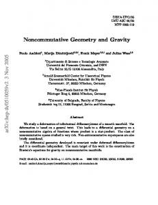
Fig. 3. Wilson string along CL and CR .
Fig. 4. Wilson string along CLR .
(35) "
)
(
(
¯ µ ΦLR = UL ∂¯µ 1 MURL + Φ˜LR − i g(W ′L + W ′R ) 1 MURL + Φ˜LR D µ µ g 2 g
)#
UR† , (36)
and ΦLR ΦRL −
1 2 1 M = M(ULR Φ˜LR + URL Φ˜RL ) + Φ˜LR Φ˜RL , g2 g
(37)
where we have used the abbreviations ULR for UL UR† , URL for UR UL† , and i Wµ′K for WµK + UK† ∂µ UK , g
(K = L, R).
(38)
From the expression (37), it is obvious that linear terms of M give rise to mass terms for the Φ˜LR field. If we decompose the Φ˜LR field into its real components in such a way that Φ˜LR = σLR + iπLR ,
Φ˜RL = σRL − iπRL ,
(39)
then one can say that σLR and πLR become massive fields, respectively, for L/R symmetric and L/R anti-symmetric configurations. As for UL and UR , it is also interesting to consider (
Z
xL
(
Z
xR
UL = P exp ig UR = P exp ig
(CL )
)
dz µ WµL (z) ,
(CR )
dz
µ
WµR (z)
)
.
(40) (41)
Here CL and CR are paths from infinitely distant places to xL and xR , respectively, (Fig. 3); according to these choices of UL and UR , ULR can be understood as �
ULR = P exp ig
Z
CLR
µ
�
dz Wµ (z) ,
(42)
where CLR is a finite path from xR to xL (Fig. 4). If it is necessary, one may define CLR as a straight line, and then, it is possible for Φ˜LR to retain its meaning as a bi-local field. 8
A particularly interesting point regarding the above choice of UL and UR is the fact that Wµ′L and Wµ′R defined in (38) vanish, and thus the action becomes very simple. If we adopt (42) to express the gauge degrees of freedom UL and UR of φLR , then the action (30) is reduced to S=−
1 2
+
Z
Z
−2g +
Z
d4 xFµν F µν
d4 xL 2
Z
Z
d4 xR ∂µ
4 L
dx
Z
4 R
dx
(
1 MULR + Φ˜LR g
! 2
¯ + 4 ∂µ
1 MULR + Φ˜LR g
� 1 � M ULR Φ˜LR + URL Φ˜RL + Φ˜LR Φ˜RL ) g
)2
! 2
d4 xΨ iγ µ (∂µ − igWµ ) Ψ Z
4 L
+gκ d x
Z
4 R
dx
(
Ψ
L
!
!
)
1 R 1 M +ULR Φ˜LR Ψ R +Ψ M +URL Φ˜RL Ψ L , g g (43)
from which we can derive the equation of motion for Φ˜LR in the following form: !
1 MULR + Φ˜LR g ( ) � 1 � +4gMURL M ULR Φ˜LR + URL Φ˜RL + Φ˜LR Φ˜RL g ( ) � 1 � 2˜ ˜ ˜ ˜ ˜ +4g ΦLR M ULR ΦLR + URL ΦRL + ΦLR ΦRL g h
∂ + 4∂¯2 2
i
R
−gκΨ URL Ψ L = 0.
(44)
If we here assume that M 2 ∝ x¯2 , then the term 4M 2 Φ˜LR in the second line of the above equation yields the mass term for Φ˜LR , which should be compared with the bi-local field R
equation (1) in the COQM model. Further, for large gκ, Ψ URL Ψ L becomes the leading term that determines Φ˜LR .
§3. Extension to a QCD-type Model The extension of the model in the previous section to a QCD-type model is not difficult, and is simply a formal task. In this case, the matter fields, the quark fields, have the L/R
components Ψi,α , where i (= 1, 2, 3) and α (= 1, 2) are the indices of color and flavor, respectively; for simplicity, we confine our attention to the case of one generation. The Higgs-like scalar fields φLR are, then, 2 × 2 matrices in flavor space and 8 × 8 matrices in 9
color space. We assume that the gauge degrees of freedom of those fields are factorized in ˜ LR U † . such a way that φLR = UL Φ R " L# Ψ , let us define the η-derivative of Ψ by Now, writing the matter fields as Ψ = R Ψ ! 0 MLR ∂η Ψ = iπΨ = −i Ψ , where MLR = UL MUR† = ULR M, and M is a function MRL 0 2 of x¯ . The meaning of η is determined by the definition of ∂η Ψ itself. With the aid of this form of iπ, it is not difficult to verify the nilpotency of the η-derivative operator (2) acting on matrices. The choice of iπ should be understood as a modified version of case (ii) in Eq. (34). According to the prescription in the previous section, first, we define the covariant derivative operators DµL/R± in this model by DµL± = (DµL ± ∂µR ) ⊗ T L ,
DµR± = (DµR ± ∂µL ) ⊗ T R
(45)
DµL/R = ∂µL/R − igWµL/R ,
(WµL/R = Wµa (xL/R )Ta ),
(46)
with where Ta (a = 1 − 8) and T L/R are generators of color gauge transformations, normalized so that tr(Ta Tb ) = 21 δa,b , and matrices defined in Eq. (6), respectively. There is no difference between the left and the right gauge fields, and hence, L and R simply designate their ˜ η are again defined by coordinate dependence. Secondly, the covariant derivatives Dη and D Dη = ∂η − ig
0 φRL
φLR 0
!
,
˜ η = −ig D
0 ΦRL
ΦLR 0
!
,
(47)
in the same way as in Eqs. (12) and (13), except that φLR and ΦLR = UL MUR† + φLR are matrix fields obeying bilinear transformations such as ΦLR → UL ΦLR UR† under gauge transformations. L/R± ± Using these covariant-derivative operators, the field strengths Fµν , Fµη and Fηη are calculated similarly as those in the previous section, and we have
i L/R Fµν = Fµν (xL/R ) ⊗ T L/R , (Fµν = [Dµ , Dν ]), g + † Fµη = (Dµ ΦLR )Q + (Dµ ΦRL )Q , o n ¯ µ ΦLR )Q + (D ¯ µ ΦRL )Q† F − = 2 (D
(48)
(49)
µη
and Fηη
)
(
1 1 = −2ig (ΦLR ΦRL − 2 M 2 ) ⊗ T L + (ΦRL ΦLR − M 2 ) ⊗ T R . g g 10
(50)
Here, Dµ ΦLR = ∂µ ΦLR − ig(WµL ΦLR − ΦLR WµR ), (51) ¯ µ ΦLR = ∂¯µ ΦLR − 1 ig(WµL ΦLR + ΦLR WµR ), D (52) 2 and the equations obtained by interchanging R and L also hold. The action for gauge and Higgs-like bi-local fields is given, again, by Eq. (28); there, we do not need the second term L/R on the right-hand side, since the Fµν represent values at different spacetime points of one field. It is also apparent that the form of the action for the matter fields coincides with that of Eq. (29). Therefore, the action in this QCD-type model should be given in the following form: 1 S=− 4Z
Z
d4 x tr Fµν F µν
+
d4 xL
−2g
2
+
Z
+gκ
Z
Z
¯ µ ΦLR D ¯ µ ΦRL d4 xR Tr Dµ ΦLR Dµ ΦRL + 4D
4 L
dx
Z
n
1 d x Tr ΦLR ΦRL − 2 M 2 g 4 R
!2
o
d4 xΨ iγ µ (∂µ − igWµ ) Ψ Z
d4 xL
Z
�
R
L
�
d4 xR Ψ ΦLR Ψ R + Ψ ΦRL Ψ L ,
(53)
where tr and Tr stand for the traces taken over color indices and over color-flavor indices, respectively. The next task is to choose a particular vacuum such that hΦLR ΦRL i0 = extension of case (ii) in the previous section, we set ΦLR = UL
(
)
1 M + (σLR + iπLR ) UR† , g
1 M 2. g2
a (πLR = πLR τa ),
As an
(54)
a where σLR = σ(xL , xR ) and πLR = π a (xL , xR ) are real fields. Then, we have
"
˜ LR − Dµ ΦLR = UL ∂µ Φ "
(
ig(Wµ′L
−
Wµ′R )
(
1 ˜ LR M +Φ g
)
)#
UR† ,
(
(55)
˜ LR − i g(W ′L + W ′R ) 1 M + Φ ˜ LR ¯ µ ΦLR = UL ∂¯µ 1 M + Φ D µ µ g 2 g
)#
UR† ,
(56)
˜ LR = σLR + iπLR and where Φ i Wµ′K = UK† WµK UK + UK† ∂µ UK , g
(K = L, R).
(57)
Further, we have )
(
� 1 1� ˜ ˜ RL M + Φ ˜ LR Φ ˜ RL U † . M ΦLR + Φ ΦLR ΦRL − 2 M 2 = UL L g g
11
(58)
In what follows, we do not distinguish Wµ′L/R and WµL/R , since the kinetic terms of gauge fields are invariant under the transformation (57). Therefore, recalling that ΦLR = Φ(xL , xR ) and ΦRL = Φ† (xR , xL ), the action (53) becomes
S=− +
1Z 4 d x tr (Fµν F µν ) 4 Z
4 L
dx
Z
4 R
dx
Tr ∂µ σLR
−
ig(WµL
−
WµR )
( ) ( � 1 i � L 1 ¯ R M + σLR − g Wµ + Wµ M + 4 ∂µ g 2 g 2 + ∂µ πLR − ig(WµL − WµR )πLR 2 ) i L R + 4 ∂¯µ πLR − g(Wµ + Wµ )πLR 2 ( Z Z
−2g 2
d4 xL
(
1 M + σLR g
) 2 + σLR
) 2
1 M(σLR + σRL ) + σLR σRL + ~πLR · ~πRL g
d4 xR T r
i + M(πLR − πRL ) + i(πLR σRL − σLR πRL ) + i(~πLR × ~πRL ) · ~τ g +
Z
)2
d4 xΨ iγ µ (∂µ − igWµ )Ψ
+gκ
Z
R
4 L
dx
+Ψ URL
Z
4 R
dx
(
!
M + σLR + iπLR Ψ R g
L
Ψ ULR !
)
M + σRL − iπRL Ψ L . g
(59)
In the action (59), neither the local color gauge symmetry nor the chiral flavor-SU(2) symmetry remains, because of its non-local property and the presence of M. In particular, a the mass terms for πLR fields arise only for π a (xL , xR ) 6= π a (xR , xL ). The form of the resultant action has a similarity to that of the linear sigma model∗) in an extended sense; a that is, if we take the local limit xL → xR , then the πLR will tend to massless Goldstone, π a meson, fields. One can see that a non-trivial potential term M 2 (¯ x) 6= 0 for σLR , πLR arises
simultaneously with the appearance of potential terms for Ψ and WµL/R . We also note that if we regard ULR as Wilson’s string function, then WµL ± WµR terms in (59) vanish; and the action will restore the color gauge invariance in appearance.
∗)
Recently, the reality of σ particle was discussed by S. Ishida. 9)
12
§4. Summary and discussion In this paper, we have discussed the possibility of extending gauge theories based on NCG to a gauge theory including bi-local Higgs-like fields. The bi-local field theories following this line are also interesting from the point of view that they are low energy examples of matrix field theories. 10) In §2, first, we reviewed Coquereaux’s formulation of the NCG within the framework of the U(1/1) gauge-Higgs model, in which the mass matrix of the matter fields, the Dirac fields, plays the role of the matrix coordinate connecting the left/right- components of matter fields at the same spacetime point. The mass parameter in the matrix coordinate determines the order of symmetry breaking. In addition, the Higgs-like fields can be understood as the quantum fluctuations around this matrix coordinate. Then, we attempted to extend such a gauge-Higgs theory to a bi-local theory by introducing a matrix coordinate that connects the left/right-components of matter-fields at different spacetime points. With this extension, the Higgs-like fields in this model become bi-local fields, while the gauge fields and the matter fields remain as local fields living in the left or in the right world. Furthermore, the mass parameter in the matrix coordinate is allowed to be a function of relative coordinates. Then it acquires the meaning of a c-number potential function for the bi-local Higgs-like fields. The extension of the toy model to a QCD-type model is rather formal, and this was done in §3 within the framework of one generation. The matter fields in this case are assumed to be (u, d)-quark fields, and the gauge structure in this model is the color gauge symmetry, which does not distinguish between the left and the right gauge fields. In this extended model, the mass parameter is introduced through the η-derivative of matter fields: (∂η )LR = −iUL MUR† , etc. Here, UL and UR are necessary to guarantee the gauge invariance of the theory before symmetry breaking. In particular, if we regard UL and UR as Wilson string functions, then the Ψ L ULR ΨR can be leading terms determining bi-local fields under a specific choice of parameters. The extended bi-local fields in this QCD-type model should be regarded as mesons, although its action contains non-local 3-body and 4-body self-interactions. The resultant action has a structure similar to that of the linear sigma model in local-chiral field theories; the mass terms, potential terms, for π-meson components vanish in the local limit xL → xR . It should be noted that if we replace M with a matrix in flavor space, such as M = a1+bτ3 , in the sense of explicit symmetry breaking, then the π ± -components of the bi-local field remain massive fields even in the local limit. It is also important that if we assume a functional form such that M 2 ∝ x¯2 , the model has a structure similar to COQM. Unfortunately, however, there is no way to determine the functional form of M 2 from this formalism. Under such an 13
assumption, further, the elimination of the relative time x¯0 becomes a serious problem, as in COQM. Also, in our approach of introducing bi-local fields ΦLR , the role of the intrinsic spins in quark-bound states is not clear. Although these problems are left as the subject of future examinations, the bi-local extension of gauge theories based on non-commutative geometry gives us an interesting insight to study the bound-state structure of matter fields. Acknowledgements The authors would like to express their sincere thanks to Professor S. Ishida and Professor S. Y. Tsai for their interest and discussions. One of the authors (S. N.) wishes to express his gratitude to the late Dr. H. Suura for his discussions in the early stage of this work. They are also grateful to Professor J. Otokozawa, Dr. S. Deguchi and other members of their laboratory for encouragement. References [1] For example, A. A. Migdal, Ann. of Phys. 126 (1980), 279. W. Lucha, F. Sch¨oberl, D. Gromes, Phys. Rep. 200 (1991), 127. See also references contained therein. [2] H. Yukawa, Phys. Rev. 91 (1953), 415, 416. [3] As for the review articles of bi-local models, see the following: T. Takabayasi, Prog. Theor. Phys. Suppl. vol. 67 (1979), 1. T. Got¯o, S. Naka and K. Kamimura, ibid, 69. T. Takabayasi, Nuovo Cim. 33 (1964), 668. [4] S. Ishida and T. Sonoda, Prog. Theor. Phys. 70 (1984), 1323. S. Ishida and M. Oda, in Proc. of the International Symposium on Extended Objects and Bound Systems, Karuizawa, Japan, 19-21 March 1992, ed. O. Hara et al. (World Scientific Pub Co., 1992), p181. [5] A. Connes and J. Lott, Nucl. Phys. B (Proc. Suppl.) 18 (1990), 29. See also A. Connes, Noncommutative Geometry (Academic Press, New York, 1994). [6] A. H. Chamseddine, G. Felder and J. Fr¨ohlich, Phys. Lett. B296 (1992), 109; Nucl. Phys. B395 (1993), 672. D. Kastler, Rev. Math. Phys. 5 (1993), 477. A. Sitarz, Phys. Lett. B308 (1993), 311. K. Morita, Prog. Theor. Phys. 90 (1993), 219. H. G. Ding, H. Y. Guo, J. M. Li and K. Wu, Z. Phys. C64 (1994), 521. 14
K. Morita and Y. Okumura, Prog. Theor. Phys. 91 (1994), 959. Y. Okumura, Prog. Theor. Phys. 92 (1994), 625. G. Konisi and T. Saito, Prog. Theor. Phys. 95 (1996), 657. See also J. Madore, Phys. Rev. D41 (1990), 3709. [7] S. Naka, E. Umezawa, T. Matsufuji, S. Abe and Y. Furukawa, Proc. of the Workshop on Fundamental Problem in Particle Physics, NUP-A-95-11. [8] R. Coquereaux, G. Esposito-Farese and G. Vaillant, Nucl. Phys. B353 (1991), 689. See also S. Naka and E. Umezawa, Prog. Theor. Phys. 92 (1994), 189. [9] S. Ishida, M. Y. Ishida, T. Ishida, K. Takamatsu and T. Tsuru, Prog. Theor. Phys. 98 (1997), 621. [10] P.-M. Ho and Y.-S. Wu, Phys. Lett. B398 (1997), 52. M. R. Douglas, hep-th/9901146. D. Bak and S.-J. Rey, hep-th/9902101. K. Hashimoto, hep-th/9903115. See also E. Witten, Nucl. Phys. B460 (1996), 335. Z. Kakushadze and S.-H. Henry Tye, hep-th/9809147.
15