Biconic aggregation functions with a given ... - ATLANTIS PRESS

EUSFLAT-LFA 2011

July 2011

Aix-les-Bains, France

Biconic aggregation functions with a given diagonal or opposite diagonal section Tarad Jwaid1 Bernard De Baets1 Hans De Meyer2 1

Dept. of Applied Mathematics, Biometrics and Process Control, Ghent University Coupure links 653, B-9000 Gent, Belgium 2 Dept. of Applied Mathematics, Computer Science, Ghent University Krijgslaan 281 S9, B-9000 Gent, Belgium

Abstract

and TD (x, y) = 0 elsewhere, are examples of tnorms. Moreover, for any semi-copula S the inequality TD ≤ S ≤ TM holds. A semi-copula S is a quasi-copula if it is 1-Lipschitz continuous, i.e. for any x, x0 , y, y 0 ∈ [0, 1] such that x ≤ x0 and y ≤ y 0 , it holds that

A new method to construct aggregation functions is introduced. These aggregation functions are called biconic aggregation functions with a given diagonal (resp. opposite diagonal) section and their construction method is based on linear interpolation on segments connecting the diagonal (resp. opposite diagonal) of the unit square and the points (0, 1) and (1, 0) (resp. (0, 0) and (1, 1)). Special classes of biconic aggregation functions such as biconic semicopulas, quasi-copulas and copulas are studied in detail.

|S(x0 , y 0 ) − S(x, y)| ≤ |x0 − x| + |y 0 − y| . A semi-copula S is a copula if it is 2-increasing, i.e. for any x, x0 , y, y 0 ∈ [0, 1] such that x ≤ x0 and y ≤ y 0 , it holds that VS ([x, x0 ] × [y, y 0 ]) := S(x0 , y 0 ) + S(x, y) − S(x0 , y) − S(x, y 0 ) ≥ 0 . VS is called the volume of the rectangle [x, x0 ] × [y, y 0 ]. Any copula is a quasi-copula since the 2-increasingness of a semi-copula implies its 1Lipschitz continuity. The (quasi-)copulas TM and TL with TL (x, y) = max(x + y − 1, 0), are respectively the greatest and the smallest (quasi-)copulas, i.e. for any (quasi-)copula C, it holds that TL ≤ C ≤ TM . The diagonal section of a [0, 1]2 → [0, 1] function F is the function δF : [0, 1] → [0, 1] defined by δF (x) = F (x, x). A diagonal function [13] is a function δ : [0, 1] → [0, 1] satisfying the following conditions:

Keywords: Aggregation function, Quasi-copula, Copula, Diagonal section, Opposite diagonal section, Linear interpolation 1. Introduction A binary aggregation function A is a [0, 1]2 → [0, 1] function satisfying the following conditions: (i) A(0, 0) = 0 and A(1, 1) = 1; (ii) for any x, x0 , y, y 0 ∈ [0, 1] such that x ≤ x0 and y ≤ y 0 , it holds that A(x, y) ≤ A(x0 , y 0 ).

(D1) δ(0) = 0, δ(1) = 1;

Aggregation functions are of great importance in many fields of application. Their most prominent uses is as logical connectives in fuzzy set theory [2]. To increase modelling flexibility, new methods to construct aggregation functions are being proposed continuously in the literature [6, 18]. Special classes of aggregation functions are of particular interest, such as semi-copulas [15, 16], triangular norms [1, 22], quasi-copulas [17, 24] and copulas [1, 25]. They are all conjunctors, in the sense that they extend the classical Boolean conjunction. Recall that an aggregation function is a semicopula if it has 1 as neutral element, i.e. A(x, 1) = A(1, x) = x for any x ∈ [0, 1]. Evidently, any semi-copula S has 0 as annihilator, i.e. S(0, x) = S(x, 0) = 0 for any x ∈ [0, 1]. A semi-copula S is a triangular norm (t-norm for short) if it is commutative and associative. The aggregation functions TM and TD given by TM (x, y) = min(x, y) and TD (x, y) = min(x, y) whenever max(x, y) = 1, © 2011. The authors - Published by Atlantis Press

(D2) δ is increasing; (D3) for all x ∈ [0, 1], it holds that δ(x) ≤ x; (D4) δ is 2-Lipschitz continuous, i.e. for all x, x0 ∈ [0, 1] it holds that |δ(x0 ) − δ(x)| ≤ 2|x0 − x| . The set of all diagonal functions will be denoted by D. The set of all [0, 1] → [0, 1] functions that satisfy conditions D1 and D2 (resp. D1, D2 and D3) will be denoted by DA (resp. DS ). The diagonal section of a copula C is a diagonal function. Conversely, for any diagonal function δ, there exists at least one copula C with diagonal section δC = δ. For instance, the copula   δ(x) + δ(y) Cδ (x, y) = min x, y, 2 67

is the greatest symmetric copula with diagonal section δ [12, 14, 26]. Similarly, the opposite diagonal section of a [0, 1]2 → [0, 1] function F is the function ωF : [0, 1] → [0, 1] defined by ωF (x) = F (x, 1 − x). An opposite diagonal function [7] is a function ω : [0, 1] → [0, 1] satisfying the following conditions:

based on linear interpolation on segments connecting the diagonal of the unit square and the points (0, 1) and (1, 0). Throughout this paper the convention 00 = 0 is assumed. For any (x, y) ∈ [0, 1]2 , we introduce in this subsection the following notations u=

(OD1) for all x ∈ [0, 1], it holds that ω(x) ≤ min(x, 1 − x);

x , 1+x−y

v=

y . 1+y−x

: Let δ ∈ DA and α, β ∈ [0, 1]. The function Aα,β δ [0, 1]2 → [0, 1] defined by

(OD2) ω is 1-Lipschitz continuous, i.e. for all x, x0 ∈ [0, 1], it holds that |ω(x0 ) − ω(x)| ≤ |x0 − x| .

Aα,β δ (x, y)

The set of all opposite diagonal functions will be denoted by O. The set of all [0, 1] → [0, 1] functions that satisfy condition OD1 will be denoted by OS . The opposite diagonal section ωC of a copula C is an opposite diagonal function. Conversely, for any opposite diagonal function ω, there exists at least one copula C with opposite diagonal section ωC = ω. For instance, the copula Fω defined by Fω (x, y) = TL (x, y) + min {ω(t) | t ∈ [min(x, 1 − y), max(x, 1 − y)]} is the greatest copula with opposite diagonal section ω [7, 23]. Note that Fω is opposite symmetric [7], i.e. Fω (x, y) − Fω (1 − y, 1 − x) = x + y − 1, for any (x, y) ∈ [0, 1]2 . Diagonal and opposite diagonal functions have been used recently to construct several subclasses of aggregation functions such as quasi-copulas and copulas [5, 7, 11, 12, 13, 14, 20]. Characteristic for the aggregation function TM is that its surface is constituted from linear segments connecting its diagonal section to the points (0, 1, 0) and (1, 0, 0). Also characteristic for TM is that its surface is constituted from linear segments connecting its opposite diagonal section to the points (0, 0, 0) and (1, 1, 1). Inspired by the above interpretation, we introduce a new method to construct aggregation functions. These aggregation functions are constructed by linear interpolation on segments connecting the diagonal (resp. opposite diagonal) of the unit square to the points (0, 1) and (1, 0) (resp. (0, 0) and (1, 1)). This paper is organized as follows. In the next section we introduce the definition of a biconic function with a given diagonal section and characterize the class of biconic aggregation functions, as well as the classes of biconic semi-copulas, biconic quasicopulas, biconic copulas and singular biconic copulas. The class of biconic functions with a given opposite diagonal section is introduced in Section 3. Finally, some conclusions are given.

=

 δ(v)   α(x − y) + y   v

, if y ≤ x ,

   β(y − x) + x δ(u) u

, otherwise

(1) is well defined. This function is called a biconic function with a given diagonal section. Proposition 1 Let δ ∈ DA . The function Aα,β δ defined in (1) is an aggregation function if and only if (i) the functions µδ,α , µδ,β : ]0, 1] → R, defined by µδ,α (x) =

δ(x) − α , x

µδ,β (x) =

δ(x) − β , x

are increasing; (ii) the functions λδ,α , λδ,β : [0, 1[ → R, defined by λδ,α (x) =

δ(x) − α , 1−x

λδ,β (x) =

δ(x) − β , 1−x

are increasing. Inspired by the above proposition, the biconic function Aα,β is called a biconic aggregation function δ with a given diagonal section. Example 1 Consider the diagonal section δM of TM , i.e. δM (x) = x for any x ∈ [0, 1]. Obviously, conditions (i) and (ii) of Proposition 1 are satisfied. The resulting biconic aggregation function is a Choquet integral [4, 10], i.e.

Aα,β δM (x, y)

=

  αx + (1 − α)y

, if y ≤ x ,

  (1 − β)x + βy

, otherwise .

Taking β = 1 − α, the resulting biconic aggregation function is the weighed arithmetic mean, i.e. Aα,1−α (x, y) = αx + (1 − α)y . δM

2. Biconic functions with a given diagonal section

Proposition 2 Let Aα,β be a biconic aggregation δ function. Then the inequality

2.1. Biconic aggregation functions with a given diagonal section

max(αx, βx) ≤ δ(x) ≤ min(α+(1−α)x, β+(1−β)x) , (2) holds for any x ∈ [0, 1].

In this subsection we introduce biconic functions with a given diagonal section. Their construction is 68

Evidently, any biconic function Aα,β is continuous if δ and only if δ is continuous. The functions δ α,β and α,β δ need not to be continuous in general. In fact, the only case in which they are both continuous is when

Now we identify the functions in DA which characterize the extreme biconic aggregation functions with fixed α and β. Let α, β ∈ [0, 1] and consider α,β : [0, 1] → [0, 1], defined by the functions δ α,β , δ

δ α,β (x)

δ

α,β

(x)

  max(αx, βx) =

, if x < 1 , max(α, β) = 1 and min(α, β) = 0 .

 

1 , if x = 1 ,   min(α + (1 − α)x, β + (1 − β)x)     , if x > 0 , =     0 , if x = 0 .

However, as Example 4 shows, it then holds that δ α,β = δ = δ

Proposition 4 Let δ ∈ DA . The function Aα,β δ defined in (1)

∈ DA and the conditions of Obviously, δ , δ Proposition 1 are satisfied. Note also that for any α,β two biconic aggregation functions Aα,β δ1 and Aδ2 , it α,β holds that Aα,β δ1 ≤ Aδ2 if and only if δ1 ≤ δ2 . The following proposition is then obvious.

α,β (i) is symmetric, i.e. Aα,β δ (x, y) = Aδ (y, x) for 2 any (x, y) ∈ [0, 1] if and only if α = β; (ii) has 0 as annihilator if and only if α = β = 0; (iii) has 1 as neutral element if and only if α = β = 0.

Proposition 3 Let Aα,β be a biconic aggregation δ function. Then it holds that

From here on, we will only consider biconic functions with a given diagonal section that have 1 as neutral element, i.e. α = β = 0. We then abbreviate A0,0 δ as Aδ . In this case, Aδ is symmetric and is given by

≤ Aα,β ≤ Aα,β Aα,β α,β . δ δ α,β δ

Example 2 The functions δ 0,0 and δ by   0 , if x < 1 , δ 0,0 (x) =

 

1

0,0

are given

Aδ (x, y) =

, if x = 1 ,

0,0

and δ (x) = x for any x ∈ [0, 1]. The corresponding biconic aggregation functions are respectively the = TD , and the greatest smallest t-norm, i.e. A0,0 δ 0,0 δ

δ

1,1

  1 (x) =

 

0

1,1

 δ(v)   y   v

, if y ≤ x ,

   x δ(u) u

, otherwise .

(3)

Suppose that the diagonal section of a biconic aggregation function Aδ contains a (linear) segment with endpoints (x1 , δ(x1 )) and (x2 , δ(x2 )). From the definition of a biconic function with a given diagonal section, it follows that Aδ is linear on the triangle T1 := ∆{(x1 ,x1 ),(x2 ,x2 ),(1,0)} as well as on the triangle T2 := ∆{(x1 ,x1 ),(x2 ,x2 ),(0,1)} . This situation is depicted in Figure 1. For any (x, y) ∈ T1 , it

t-norm, i.e. A0,0 0,0 = TM . Example 3 The functions δ 1,1 and δ by δ 1,1 (x) = x for any x ∈ [0, 1] and

= δM ,

and Aα,β coincides with one of the projections. δ

α,β

α,β

α,β

are given

, if x > 0 , , if x = 0 .

The corresponding biconic aggregation functions are respectively the smallest t-conorm, i.e. (x, y) = max(x, y), and the greatest t-conorm, A1,1 δ 1,1 i.e. A1,1 1,1 (x, y) = max(x, y) whenever min(x, y) = 0, δ

and A1,1 1,1 (x, y) = 1 elsewhere. δ

1,0

Example 4 The functions δ 1,0 , δ , δ 0,1 and 0,1 δ all coincide with δM . The corresponding biconic aggregation functions coincide with the projection to the first and second coordinate [2, 3], i.e. 0,1 (x, y) = A1,0 A1,0 1,0 (x, y) = x and Aδ 0,1 (x, y) = δ 1,0 A0,1 0,1 (x, y) = y.

Figure 1: Illustration for the triangles T1 and T2 .

holds that

δ

Aδ (x, y) = ax + by + c .

δ

69

(4)

2.3. Biconic quasi-copulas with a given diagonal section

Furthermore, ax1 + bx1 + c = δ(x1 ) ax2 + bx2 + c = δ(x2 ) a + c = 0.

An interesting class of aggregation functions is the class of quasi-copulas. Quasi-copulas are of increasing importance in various studies in fuzzy set theory, such as preference modelling and similarity measurement [8, 9]. Next we characterize the diagonal functions for which the corresponding biconic function is a quasicopula.

Solving this system of equations and using the symmetry of Aδ , we obtain

Aδ (x, y) =

 rx + sy − r     t

, if (x, y) ∈ T1 ,

    sx + ry − r t

, if (x, y) ∈ T2 ,

(5)

Lemma 2 Let δ ∈ D. Then it holds that (i) the function νδ : ]0, 1] → [2, ∞[ , defined by , is decreasing; νδ (x) = 1+δ(x) x (ii) the function φδ : [0, 1/2[ ∪ ]1/2, 1] → R, defined δ(x) , is increasing on the interval by φδ (x) = 1−2x [0, 1/2[ and on the interval ]1/2, 1].

where r = x1 δ(x2 ) − x2 δ(x1 ) s = (1 − x1 )δ(x2 ) − (1 − x2 )δ(x1 )

Proposition 7 Let δ ∈ D. Then the function Aδ : [0, 1]2 → [0, 1] defined in (3) is a quasi-copula if and only if

t = x2 − x1 . 2.2. Biconic semi-copulas with a given diagonal section

(i) the function µδ , defined in Proposition 5, is increasing; (ii) the function ξδ : [0, 1[ → [0, 1[ , defined by ξδ (x) = x−δ(x) 1−x , is increasing.

In this subsection we characterize the set of functions in DS for which the corresponding biconic function is a semi-copula.

Example 7 Consider the diagonal function in Example 6. Clearly, the functions µδ and ξδ , defined in Propositions 5 and 7, are increasing. The corresponding family of biconic semi-copulas is a family of biconic quasi-copulas.

Lemma 1 Let δ ∈ DS . The function λδ : [0, 1[ → δ(x) , is increasing; [0, ∞[ , defined by λδ (x) = 1−x Proposition 5 Let δ ∈ DS . Then the function Aδ : [0, 1]2 → [0, 1] defined in (3) is a semi-copula if and only if the function µδ : ]0, 1] → [0, ∞[ , defined by µδ (x) = δ(x) x , is increasing.

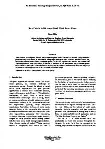
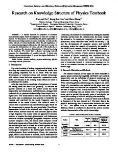
Example 8 Consider the fined by   0       1   2x − 3 δ(x) =  2   x    3    2x − 1

Example 5 Consider the diagonal functions δM and δL with δL being the diagonal section of TL , i.e. δL (x) = max(2x − 1, 0) for any x ∈ [0, 1]. Clearly, the functions µδM and µδL , defined in Proposition 5, are increasing. The corresponding biconic semicopulas are respectively TM and TL .

Aθ (x, y) =

    

x1+θ (1 + x − y)θ

, if x ≤

1 6

,

, if

1 6

≤x≤

1 4

,

, if

1 4

≤x≤

3 4

,

, otherwise .

Clearly, the function µδ , defined in Proposition 5, is increasing. Note also that the function ξδ , defined in Proposition 7, is not increasing. Hence, the corresponding biconic semi-copula is a proper semicopula. Consequently, the class of biconic quasicopulas with a given diagonal section is a proper subclass of the class of biconic semi-copulas with a given diagonal section.

Example 6 Consider the diagonal function δ(x) = x1+θ with θ ∈ [0, 1]. Clearly, the function µδ , defined in Proposition 5, is increasing for any θ ∈ [0, 1]. The corresponding family of biconic semicopulas is given by  y 1+θ      (1 + y − x)θ

diagonal function δ de-

, if y ≤ x ,

Proposition 8 Let Aδ be a biconic quasi-copula. Then it holds that

, otherwise .

(i) if δ(x0 ) = x0 for some x0 ∈ ]0, 1[ , then Aδ = TM ; (ii) if δ(x0 ) = 2x0 − 1 for some x0 ∈ [1/2, 1[ , then δ(x) = 2x − 1 for any x ∈ [x0 , 1].

Proposition 6 Let Aδ be a biconic semi-copula and suppose that δ(x0 ) = x0 for some x0 ∈ ]0, 1[ . Then it holds that δ(x) = x for any x ∈ [x0 , 1]. 70

Example 10 Consider the diagonal function given x2 Clearly, δ by δ(x) = 1−θ(1−x) 2 with θ ∈ [−1, 1] . is convex for any θ ∈ [−1, 1] . The corresponding family of biconic copulas is given by  y 2 (1 + y − x)   , if y ≤ x ,    (1 + y − x)2 − θ(1 − x)2 Cθ (x, y) =   x2 (1 + x − y)   , otherwise .  (1 + x − y)2 − θ(1 − y)2

1 1 0.8

0.8 0.6

δ (x)

0.6 0.4 0.4

0.2 0 1

0.2

0.8

1 0.6

0

0

0.2

0.4

0.6

x

0.8

1

0.4

0.5 0.2 0

0

Example 11 Consider the given by   0 ,       1    (4x − 1) , δ(x) = 3  1   x ,    2    2x − 1 ,

Figure 2: The diagonal function and the corresponding biconic semi-copula of Example 8. 2.4. Biconic copulas with a given diagonal section Another relevant class of aggregation functions is the class of copulas. Due to Sklar’s theorem [27], copulas have received increasing attention from researchers in statistics and probability theory [19]. We denote the (linear) segment with endpoints x, y ∈ [0, 1]2 as

diagonal function δ if x ≤

1 4

,

if

1 4

≤x≤

2 5

,

if

2 5

≤x≤

2 3

,

otherwise .

Clearly, the functions µδ and ξδ , defined in Propositions 5 and 7, are increasing. Note also that δ is not convex. Hence, Aδ is a proper biconic quasicopula. Consequently, the class of biconic copulas

hx, yi = {θx + (1 − θ)y | θ ∈ [0, 1]} . Proposition 9 Let δ be a piecewise linear diagonal function. Then the function Aδ : [0, 1]2 → [0, 1] defined in (3) is a copula if and only if δ is convex.

1 1

0.8

0.8

0.6 0.6

δ(x)

Lemma 3 Let Cδ be a biconic copula and m1 , m2 ∈ ] − ∞, 0[ such that m1 > m2 . Consider three points b1 := (x1 , x1 ), b2 := (x2 , x2 ) and b3 := (x3 , x3 ) such that 0 ≤ x1 < x2 < x3 ≤ 1 and the segments hb1 , (1, 0)i, hb2 , (1, 0)i and hb3 , (1, 0)i have slopes √ m1 , − m1 m2 and m2 , respectively. Then it holds that

0.4

0.4 0.2

0 1

0.2

0.8 0

1 0.6

0

0.2

0.4

0.6

x

0.8

1

0.8 0.6

0.4 0.4

0.2

0.2 0

0

Figure 3: The diagonal function and the corresponding biconic quasi-copula of Example 11.

(i) there exists a rectangle [x, x0 ] × [y, y 0 ] such that the segment connecting the points (x, y 0 ) and (x0 , y) is a subset of the segment hb2 , (1, 0)i and the points (x, y) and (x0 , y 0 ) are located on the segments hb1 , (1, 0)i and hb3 , (1, 0)i respectively. (ii) the point (x2 , δ(x2 )) lies below or on the segment h(x1 , δ(x1 )), (x3 , δ(x3 ))i.

with a given diagonal section is a proper subclass of the class of biconic quasi-copulas with a given diagonal section. In the following lemma the opposite symmetry property of a biconic copula with a given diagonal section is studied.

Lemma 3 and Proposition 9 are used to show that for any convex diagonal function, the function Aδ defined in (3) is a copula.

Proposition 11 A biconic copula Cδ is opposite symmetric if and only if the function f (x) = x−δ(x) is symmetric with respect to the point (1/2, 1/2), i.e. δ(x) − δ(1 − x) = 2x − 1 for any x ∈ [0, 1/2].

Proposition 10 Let δ ∈ D. Then the function Aδ : [0, 1]2 → [0, 1] defined in (3) is a copula if and only if δ is convex.

Next we characterize the class of singular biconic copulas with a given diagonal section. The support of a copula C is the complement of the union of all non-degenerated open rectangles of the unit square such that the C-volume of the closed rectangle is equal to zero. A copula C is called singular if its support has Lebesgue measure zero.

Example 9 Consider the diagonal function in Example 6. Clearly, δ is convex for any θ ∈ [0, 1]. The corresponding family of biconic semi-copulas is a family of biconic copulas. 71

3. Biconic functions with a given opposite diagonal section

Proposition 12 Let Cδ be a biconic copula. Then it holds that Cδ is singular if and only if δ is piecewise linear.

In this section we introduce biconic functions with a given opposite diagonal section. Their construction is based on linear interpolation on segments connecting the opposite diagonal of the unit square and the points (0, 0) and (1, 1). For any (x, y) ∈ [0, 1]2 , we introduce in this section the following notations

Example 12 The family of biconic copulas given in (7) is a family of singular biconic copulas. We focus now on associative biconic copulas with a given diagonal section and conclude that the only two associative biconic copulas with a given diagonal section are TM and TL . Every 1-Lipschitz tnorm is a copula, while every associative copula is a t-norm (the commutativity can be obtained from the continuity of a copula [22]).

u0 =

v0 =

1−y . 2−x−y

Let ω : [0, 1] → [0, 1] and α, β ∈ [0, 1]. The function Aα,β : [0, 1]2 → [0, 1] defined by Aα,β ω ω (x, y) =  0 ω(u )   , if x + y ≤ 1 , α(1 − x − y) + x   u0

Proposition 13 TM and TL are the only biconic associative copulas (1-Lipschitz t-norms) with a given diagonal section.

 0   β(x + y − 1) + (1 − y) ω(v ) 0 v

We conclude this subsection by finding the intersection between the set of biconic copulas with a given diagonal section and the set of conic copulas. Conic copulas were introduced in [21] and their construction was based on linear interpolation on segments connecting the upper boundary curve of the zero-set and the point (1, 1). In other words, the surface of any conic copula is constituted from its zero-set and segments connecting the upper boundary curve of its zero-set to the point (1, 1, 1). The zero-set ZC of a copula C is the inverse image of the value 0, i.e.  ZC := C −1 ({0}) = (x, y) ∈ [0, 1]2 | C(x, y) = 0 .

, otherwise .

(8) is well defined. This function is called a biconic function with a given opposite diagonal section. Evidently, the boundary conditions of an aggregation function imply that α = 0 and β = 1. We then abbreviate A0,1 ω as Aω with Aω (x, y) =  0 ω(u )  x , if x + y ≤ 1 ,   u0 (9)  0  ω(v )  x + y − 1 + (1 − y) , otherwise . v0 Clearly, the function Aω defined in (9) has 1 as neutral element. Therefore, if Aω is an aggregation function then it is also a semi-copula. In the next proposition, we characterize the functions in OS for which the corresponding biconic function is a biconic aggregation function.

Lemma 4 Let δ ∈ D and suppose that θ = 1 − 1 2− θ1 , with θ1 ∈ [1, ∞[, is the maximum value such that δ(θ) = 0. Then the biconic copula Cδ has the zero set ZCδ given by

Proposition 15 Let ω ∈ OS . Then the function Aω : [0, 1]2 → [0, 1] defined in (9) is an aggregation function if and only if

ZCδ = {(x, y) ∈ [0, 1]2 | y ≤ fθ1 (x)} where the function fθ1 : [0, 1] → [0, 1] is given by  1 1 (1 − 2 θ1 )−1 x + 1 , if x ≤ 1 − 2− θ1 , fθ1 (x) = 1 1  , if x ≥ 1 − 2− θ1 . (1 − 2 θ1 )(x − 1) (6)

(i) the functions µω , ρω : ]0, 1] → [0, 1], defined by 1−ω(x) , are decreasing; µω (x) = ω(x) x , ρω (x) = x (ii) the functions λω , ξω : [0, 1[ → [0, 1], defined by x−ω(x) λω (x) = ω(x) 1−x and ξω = 1−x , are increasing. Let C be a quasi-copula (resp. copula) with opposite diagonal section ω. The function C 0 , defined by C 0 (x, y) = x−C(x, 1−y), is again a quasi-copula (resp. copula) whose diagonal section δC 0 is given by δC 0 (x) = x − ω(x). This transformation permits to derive in a straightforward manner the conditions that have to be satisfied by an opposite diagonal function to obtain a biconic quasi-copula (resp. copula), which has that opposite diagonal function as opposite diagonal section.

Due to the above lemma and the definition of a conic copula, the following proposition is obvious. Proposition 14 Let Cδ be a biconic copula and suppose further that Cδ is a conic copula. Then it holds that Cδ (x, y) =  1 θ   max(y + (1 − x)(1 − 2 1 ), 0) , if y ≤ x ,   max(x + (1 − y)(1 − 2 θ11 ), 0)

x , x+y

(7)

Proposition 16 Let ω ∈ O. Then the function Aω : [0, 1]2 → [0, 1] defined in (9) is a quasicopula if and only if the functions µω and λω , defined in Proposition 15, are respectively decreasing and increasing.

, otherwise ,

with θ1 ∈ [1, ∞[ . This family of copulas was introduced in [21]. 72

Proposition 17 Let ω ∈ O. Then the function Aω : [0, 1]2 → [0, 1] defined in (9) is a copula if and only if ω is concave.

4. Conclusion We have introduced biconic aggregation functions with a given diagonal (resp. opposite diagonal) section. We have also characterized the classes of biconic semi-copulas, quasi-copulas and copulas with a given diagonal (resp. opposite diagonal) section. The t-norms TM and TL turn out to be the only 1-Lipschitz biconic t-norms with a given diagonal section. Moreover, a copula that is a biconic copula with a given diagonal section as well as with a given opposite diagonal section turns out to be a convex combination of TM and TL .

Example 13 Consider the opposite diagonal functions ωM (x) = min(x, 1 − x) and ωL (x) = 0. Obviously, ωM and ωL are concave functions. The corresponding biconic copulas are respectively TM and TL . Example 14 Consider the opposite diagonal function ωΠ (x) = x(1 − x). Obviously, ωΠ is concave. The corresponding biconic copula is given by  0  x(1 − u ) CωΠ (x, y) =

 

, if x + y ≤ 1 ,

x − (1 − y)v 0

References , otherwise . [1] C. Alsina, M.J. Frank and B. Schweizer, Associative Functions: Triangular Norms and Copulas, World Scientific, Singapore, 2006. [2] G. Beliakov, A. Pradera and T. Calvo, Aggregation Functions: a Guide for Practitioners, Studies in Fuzziness and Soft Computing, Vol. 221, Springer, Berlin, 2007. [3] T. Calvo, A. Kolesárová, M. Komorníková and R. Mesiar, Aggregation Operators: Properties, Classes and Construction Methods. In: Aggregation Operators, New Trends and Applications, Physica-Verlag, New York, 2002, pp. 3– 106. [4] G. Choquet, Theory of capacities, Annales Institute Fourier, 5:131–295, 1953. [5] B. De Baets, H. De Meyer and R. Mesiar, Asymmetric semilinear copulas, Kybernetika 43:221–233, 2007. [6] B. De Baets, H. De Meyer and R. Mesiar, Piecewise linear aggregation functions based on triangulation, Information Sciences, 181:466– 478, 2011. [7] B. De Baets, H. De Meyer and M. ÚbedaFlores, Opposite diagonal sections of quasicopulas and copulas, Internat. J. Uncertainty, Fuzziness and Knowledge-Based Systems, 17:481–490, 2009. [8] B. De Baets and J. Fodor, Additive fuzzy preference structures: the next generation, in: Principles of Fuzzy Preference Modelling and Decision Making (B. De Baets and J. Fodor, eds.), Academia Press, 2003, pp. 15–25. [9] B. De Baets, S. Janssens and H. De Meyer, On the transitivity of a parametric family of cardinality-based similarity measures, Internat. J. Approximate Reasoning, 50:104–116, 2009. [10] D. Denneberg, Non-additive Measure and Integral, Kluwer, 1994. [11] F. Durante and P. Jaworski, Absolutely continuous copulas with given diagonal sections, Communications in Statistics: Theory and Methods, 37:2924–2942, 2008.

We focus now on the symmetry and opposite symmetry properties of biconic copulas with a given opposite diagonal section. Proposition 18 Let Cω be a biconic copula. Then it holds that (i) Cω is opposite symmetric; (ii) Cω is symmetric if and only if ω is symmetric with respect to the point (1/2, 1/2), i.e. ω(x) = ω(1 − x) for any x ∈ [0, 1/2] . We conclude this section by finding the intersection between the class of biconic copulas with a given opposite diagonal section and the class of biconic copulas with a given diagonal section and the class of conic copulas. Proposition 19 Let C be a biconic copula with a given opposite diagonal section and suppose further that C is a biconic copula with a given diagonal section. Then it holds that C is a member of the following family θTM + (1 − θ)TL

with θ ∈ [0, 1] .

Let Cω be a biconic copula. Due to the definition of Cω , the only possible zero-sets are ZCω = ZTM = [0, 1]2 \ ]0, 1]2 and ZCω = ZTL = {(x, y) ∈ [0, 1]2 | x + y ≤ 1} . Recalling that every conic copula is uniquely determined by its zero-set [21], the following proposition is clear. Proposition 20 Let Cω be a biconic copula with given opposite diagonal section ω and suppose further that Cω is a conic copula. Then it holds that Cω = TM or Cω = TL . 73

[12] F. Durante, A. Kolesárová, R. Mesiar and C. Sempi, Copulas with given diagonal sections, novel constructions and applications, Internat. J. Uncertainty, Fuzziness and KnowledgeBased Systems, 15:397–410, 2007. [13] F. Durante, A. Kolesárová, R. Mesiar and C. Sempi, Semilinear copulas, Fuzzy Sets and Systems, 159:63–76, 2008. [14] F. Durante, R. Mesiar and C. Sempi, On a family of copulas constructed from the diagonal section, Soft Computing, 10:490–494, 2006. [15] F. Durante, J.J. Quesada Molina and C. Sempi, Semicopulas: characterizations and applicability, Kybernetika, 42:287–302, 2006. [16] F. Durante and C. Sempi, Semicopulae, Kybernetika, 41:315–328, 2005. [17] C. Genest, J.J. Quesada Molina, J.A. Rodríguez Lallena and C. Sempi, A characterization of quasi-copulas, Journal of Multivariate Analysis, 69:193–205, 1999. [18] M. Grabisch, J.-L. Marichal, R. Mesiar and E. Pap, Aggregation functions: construction methods, conjunctive, disjunctive and mixed classes, Information Sciences, 181:23–43, 2011. [19] H. Joe, Multivariate Models and Dependence Concepts, Chapman & Hall, London, 1997. [20] T. Jwaid, B. De Baets and H. De Meyer, Orbital semilinear copulas, Kybernetika 45:1012– 1029, 2009. [21] T. Jwaid, B. De Baets, J. Kalická and R. Mesiar, Conic aggregation functions, Fuzzy Sets and Systems 167:3–20, 2011. [22] E.P. Klement, R. Mesiar and E. Pap, Triangular Norms, Trends in Logic, Studia Logica Library, Vol. 8, Kluwer Academic Publishers, Dordrecht, 2000. [23] E.P. Klement and A. Kolesárová, Extension to copulas and quasi-copulas as special 1Lipschitz aggregation operators, Kybernetika, 41:329–348, 2005. [24] A. Kolesárová, 1-Lipschitz aggregation operators and quasi-copulas, Kybernetika, 39:615– 629, 2003. [25] R. Nelsen, An Introduction to Copulas, Springer, New York, 2006. [26] R. Nelsen and G. Fredricks, Diagonal copulas. In: V. Beneš and J. Štěpán, Eds., Distributions with given Marginals and Moment Problems, Kluwer Academic Publishers, Dordrecht, 1977, pp. 121–127. [27] A. Sklar, Fonctions de répartition à n dimensions et leurs marges, Publ. Inst. Statist. Univ. Paris, 8:229–231, 1959.

74