Bidirectionalization Transformation Based on Automatic Derivation of

Bidirectionalization Transformation Based on Automatic Derivation of View Complement Functions Kazutaka Matsuda†

Zhenjiang Hu†

Keisuke Nakano†

†

The University of Tokyo [email protected] {hu,ksk,takeichi}@mist.i.u-tokyo.ac.jp

Makoto Hamana‡

Masato Takeichi†

‡

Gunma University [email protected]

Abstract

1. Introduction

Bidirectional transformation is a pair of transformations: a view function and a backward transformation. A view function maps one data structure called source onto another called view. The corresponding backward transformation reflects changes in the view to the source. Its practically useful applications include replicated data synchronization, presentation-oriented editor development, tracing software development, and view updating in the database community. However, developing a bidirectional transformation is hard, because one has to give two mappings that satisfy the bidirectional properties for system consistency. In this paper, we propose a new framework for bidirectionalization that can automatically generate a useful backward transformation from a view function while guaranteeing that the two transformations satisfy the bidirectional properties. Our framework is based on two known approaches to bidirectionalization, namely the constant complement approach from the database community and the combinator approach from the programming language community, but it has three new features: (1) unlike the constant complement approach, it can deal with transformations between algebraic data structures rather than just tables; (2) unlike the combinator approach, in which primitive bidirectional transformations have to be explicitly given, it can derive them automatically; (3) it generates a view update checker to validate updates on views, which has not been well addressed so far. The new framework has been implemented and the experimental results show that our framework has promise.

There are many situations in which one data structure, called source, is transformed to another, called view, in such a way that changes on the view can be transformed back to those on the original data structure. This is called bidirectional transformation, and practical examples include synchronization of replicated data in different formats (Foster et al. 2005), presentation-oriented structured document development (Hu et al. 2004), interactive user interface design (Meertens 1998), coupled software transformation (L¨ammel 2004), and the well-known view updating mechanism which has been intensively studied in the database community (Bancilhon and Spyratos 1981; Dayal and Bernstein 1982; Gottlob et al. 1988; Hegner 1990; Lechtenb¨orger and Vossen 2003). To be concrete, suppose that we have a list of students and professors (the source), and we want to create a view that consists of all the students. This view can be defined by the following view function.

Categories and Subject Descriptors I.2.2 [Artificial Intelligence]: Automatic Programming—Program transformation, Program synthesis; D.1.1 [Programming Techniques]: Applicative (Functional) Programming; H.2.3 [Database Management]: Language—Data manipulation languages, Query languages General Terms Languages, Design Keywords Bidirectional Transformation, View Updating, Program Transformation, Automatic Program Generation, Program Inversion.

Permission to make digital or hard copies of all or part of this work for personal or classroom use is granted without fee provided that copies are not made or distributed for profit or commercial advantage and that copies bear this notice and the full citation on the first page. To copy otherwise, to republish, to post on servers or to redistribute to lists, requires prior specific permission and/or a fee. ICFP ’07, 1–3, October 2007, Freiburg, Germany. c 2007 ACM 978-1-59593-815-2/07/0010. . . $5.00 Copyright °

students : Source → View students [ ] = [ ] students (Student name grade major : ms) = Student name grade major : students ms students (Prof name position major : ms) = students ms To develop a bidirectional transformation, in addition to the view function one needs to define another function, a backward transformation function, which is used for view updating, i.e., reflects changes on the view (such as modification of students’ names) to the source. The following function students B 1 is a backward transformation that accepts a changed view and the original source and produces a new source. students B : (Source × View) → Source students B ([ ], [ ]) = [ ] students B (Student n g m : ms, Student n0 g 0 m0 : ss) = Student n0 g 0 m0 : students B (ms, ss) students B (Prof n p m : ms, ss) = Prof n p m : students B (ms, ss) However, there are several limitations in manually writing a pair of view function and backward transformation (such as students and students B ) to develop a bidirectional transformation. First, it is difficult to prove that the two functions satisfy the bidirectional property and form a bidirectional transformation (Section 2). Second, the consistency of the two functions is difficult to maintain. A small change in the view function may require a big change in the backward transformation function. For instance, suppose we want a view that contains only the names of the students who major in 1 The

subscript B stands for “backward”.

Computer Science. While it is easy to give the following view function by composing another function with above the view function, it requires more thinking to write a backward transformation. cs cs cs cs

students = cs ◦ students [] = [] (Student name grade CS : ss) = name : cs ss ( : ss) = cs ss

Third, it is hard to automatically infer permitted changes in the view. Backward transformation functions, such as students B , are usually partial functions, disallowing some changes to the view. For example, students B does not allow insertion of a new student to the view. When the source and the view are huge, it is better to have an inference system for validating view changes rather than to directly compute backward transformation until an error message appears. Several methods for automatically deriving backward transformation functions from view definition functions have been proposed to overcome these three problems. In the database community, this issue, known as view updating problem, has been studied for a long time (Bancilhon and Spyratos 1981; Dayal and Bernstein 1982; Gottlob et al. 1988; Hegner 1990; Lechtenb¨orger and Vossen 2003). One known approach (Bancilhon and Spyratos 1981) is to construct an injective function from the view function so that changes on the image of the injective function can be reflected back to its domain by inversion. To do this, lost information in the view generation is gathered as a complement for later backward transformation. Bancilhon and Spyratos proposed the concept of view complement function and the method of view updating under constant complement. Generally speaking, for a view function from a source to a view f :S→V a view complement function of f is a function from the source to another view (called a complement view) g :S →V0 such that the tupled function (f M g) : S → (V × V 0 ) is injective. This view complement function, g, provides the information that does not appear in the view generated by f . Then, for an original source s, the updated source s0 corresponding to an updated view v can be calculated by s0 = (f M g)−1 (v, g(s)). Therefore, if a view complement function g can be derived and the inversion of (f M g) can be calculated, that means we know how to reflect changes on the view to the source. Since the derived backward transformation depends on g, we should choose an appropriate g. For example g = id S is the worst one because the derived backward transformation is defined only on the input (s, v) by v = f (s), i.e., no updates are allowed. This approach has been applied to solving the view updating problem in the relational database system (Cosmadakis and Papadimitriou 1984; Laurent et al. 2001; Lechtenb¨orger and Vossen 2003). In fact, derivation of view complement functions and inversion calculation are simplified in the context of relational databases because views and sources are sets of flat tuples, and view functions are queries in a simple form being closed under composition. However, though tree-structured data, e.g. XML, is now widely used, how to apply the approach to view functions that can deal with general algebraic data structures such as trees is still an open problem. The challenge is to find a suitable form for these view functions such that they not

only have enough descriptive power and view complement functions but are suitable for later inversion calculation. Another approach, which has received increasing attention in recent years, is to design a set of general combinators (Foster et al. 2005; Hu et al. 2004; Meertens 1998) for constructing bigger bidirectional transformations by composing smaller ones. A set of primitive bidirectional transformations, each being defined by a pair of view function and backward transformation, is prepared, and a new bidirectional transformation is defined by assembling the primitive transformations with a fixed set of general combinators (Section 2.4.2). This approach has proved to be practically useful for domain-specific applications, because primitive bidirectional transformations for a specific application are easily determined, designed, and implemented. Moreover, this approach is general and can deal with trees other than relational tables provided that suitable primitive bidirectional transformations on trees are given. However, for an involved application or in a more general setting, a lot of primitive bidirectional transformations may need to be prepared, and it is still hard to verify whether a pair consisting of a view function and a backward transformation forms a (primitive) bidirectional transformation. In this paper, we propose a new bidirectional transformation framework that combines the advantages of the above two approaches: automatic bidirectionalization and ability to deal with tree structures. We follow the combinator approach of keeping separate the design of primitive bidirectional transformations and the design of composition methods for gluing smaller transformations, but we borrow the idea of the view complement approach to obtain primitive bidirectional transformations that can manipulate arbitrary algebraic data structures. The key to our framework is a suitable language for describing primitive view functions. It should be sufficiently powerful to specify various view functions over algebraic data structures, simple enough for derivation of view complement functions and inversion, and suitable for use as components to be composed with others. We choose a general first-order functional language and require view functions that are defined in the language to be affine (each variable is used at most once) and in the treeless form (no intermediate data structure is used in the definition). In fact, this class of functions has been considered elsewhere in the context of deforestation (fusion transformation) (Wadler 1990), where treeless functions are used to describe basic computation components. In our framework, view complement functions can be automatically derived from view functions, and the derived view complement functions are suitable for tupling and inversion. Moreover, updatability of views can be represented by a regular tree language with which one can statically check whether changes in views are valid or not without really performing backward transformation. We have implemented all the ideas in this paper using a bidirectionalizing system for automatically constructing backward transformation functions from view functions. The derived backward transformation function is correct in the sense that it forms a bidirectional transformation with the view function, useful in the sense that all the tracing information between the source and the view is recorded in such a way that any change in the view element that has a corresponding element in the source can be reflected to the source, powerful in the sense that it can deal with bidirectional transformation between arbitrary algebraic data structures such as lists and trees, and equipped with an inference system for validating changes in the view. This paper is organized as follows. We start by explaining the basic concepts of bidirectional transformation in Section 2. Then, after presenting an overview of our system in Section 3, we define a language for view definition in Section 4, show how to derive view complement functions in Section 5, explain how to generate

backward transformation functions based on tupling and inversion in Section 6, and give an algorithm for updatability check in Section 7. We illustrate the whole bidirectionalization procedure with a concrete example in Section 8. Finally, we discuss related work in Section 9, and conclude the paper and highlight some future directions in Section 10. For proofs (of all theorems), which are omitted in this paper, please see Matsuda et al. (2007).

translated to an update on sources of s ½ ρ(s, v), and ρ(s, v) = ⊥ means that it prohibits the view update f (s) ½ v. Moreover, backward transformation functions are not unique, and different definitions give different translation policies. For instance, the following is a backward transformation function of the view function mapfst:  s if v = mapfst(s) ρ(s, v) = ⊥ otherwise,

2.

which means that any change in the view is ignored and the source remains unchanged.

Bidirectional Transformation

In this section, we briefly review notations, the basic concept of bidirectional transformation (i.e., view updating) (Bancilhon and Spyratos 1981; Dayal and Bernstein 1982; Gottlob et al. 1988; Hegner 1990; Lechtenb¨orger and Vossen 2003; Foster et al. 2005), and the technique of bidirectionalization based on derivation of view complement functions (Bancilhon and Spyratos 1981). These will serve as the basis of our approach. 2.1

Notations

Our notations, if not explained, follow Haskell2 , a functional programming language. For a partial function f , we write f (x)↓ if f (x) is defined, and write f (x) = ⊥ otherwise. For a function f : X → Y and a function g : X → Z, we define a tupled function (f M g) : X → (Y × Z) by (f M g)(x) = (f (x), g(x)). For a partial function f : X → Y and a partial function g : X → Y , we write f v g to denote ∀x ∈ X, f (x)↓ ⇒ f (x) = g(x). Intuitively, f v g means that g is more widely defined than f . 2.2 View Function and Backward Transformation Let V be the set of views and S be the set of sources. A total function f : S → V that constructs a view from a source is called view function. The following is an example of a view function mapfst(Nil) mapfst(Cons(Pair(a, b), x))

= =

Nil Cons(a, mapfst(x))

that maps the source, a list of pairs, to the view, a list that contains all the first components of the pairs in the original list. A function that translates an update on views to that on sources is called a backward transformation function. An update from x to x0 is denoted as x ½ x0 ; e.g., Nil ½ Cons(A, Nil) represents the update on the view of mapfst from Nil to Cons(A, Nil). Given a view function f : S → V , a backward transformation function ρ : (S × V ) → S of f translates f (s) ½ v, an update on views, to s ½ ρ(s, v), an update on sources, while satisfying the property: ∀s ∈ S, ∀v ∈ V, ρ(s, v)↓ ⇒ f (ρ(s, v)) = v. This property reads that the updated source produced by the backward transformation should not change the view with the view function. In other words, for a source element s and v = f (s), let u be a view update v ½ v 0 and u0 a translated source update s ½ ρ(s, v 0 ), then the following diagram commutes. u V -V f6

6 f

-S u0 It might be easier to understand a backward transformation function ρ : (S ×V ) → S as a mapping that accepts an original source and a changed view as input and produces a changed source as the result. It is worth noting that backward transformation functions are partial: ρ(s, v)↓ means that an update on views of f (s) ½ v is S

2 Haskell

98 Report: http://www.haskell.org/onlinereport/

2.3

Bidirectional Properties

A backward transformation function ρ and a view function f should satisfy some bidirectional properties to guarantee consistency after bidirectional transformation is carried out. The following properties follow those in the closed view updating (Bancilhon and Spyratos 1981; Hegner 1990), where the source is completely hidden from the users when the view is updated. Let s ∈ S and v, v 0 ∈ V . A backward transformation function ρ : (S × V ) → S and a view function f : S → V should satisfy the following bidirectional properties. ACCEPTABILITY ρ(s, f (s)) = s U NDOABILITY ρ(s, v)↓ ⇒ ρ(ρ(s, v), f (s)) = s C OMPOSABILITY ρ(s, v)↓ ∧ ρ(ρ(s, v), v 0 )↓ ⇒ ρ(ρ(s, v), v 0 ) = ρ(s, v 0 ) Acceptability means that if there is no change in views there should be no change in sources. Undoability means that all translated updates can be canceled by updates on views. Composability means that the update translation should preserve the compositional structure3 , and translated results do not depend on the update history. 2.4 Bidirectionalization Bidirectionalization is a program transformation that derives a backward transformation function from a view function such that the two functions satisfy the bidirectional properties. It is very much related to the known view update problem in the database community, which discusses how to translate updates on views to updates on sources. We shall review two approaches on which our method is based. 2.4.1

Constant Complement Approach

Bancilhon and Spyratos (1981) proposed a general approach to bidirectionalization called constant complement view updating. Definition 1 (View Complement Function). A function g : S → V 0 is said to be a (view) complement function to a view function f : S → V , if the tupled function f M g : S → (V × V 0 ) is injective. Intuitively, a view complement function of a view function provides information that is not visible in the view to a complement view such that information from both views can uniquely determine a source. For example, let add be a function defined by add (x, y) = x+y. Then, the function fst defined by fst(x, y) = x is a view complement function of add . Note that the ranges of view function f and its complement function g can be different. In fact, 3 Note that u = f (s)½v is translated to u0 = s½ρ(s, v), u = v ½v 0 1 2 1 is translated to u02 = ρ(s, v) ½ ρ(ρ(s, v), v 0 ), and their composition 0 0 u = u1 ◦ u2 = f (s) ½ v is translated to u = s ½ ρ(s, v 0 ) = s ½ ρ(ρ(s, v), v 0 ) = u01 ◦ u02 .

the range of the view complement function is unimportant. This gives us freedom in derivation of view complement functions. Finding a view complement function of a view function amounts to bidirectionalization, provided that inversion of can be calculated out (Bancilhon and Spyratos 1981). If a view complement function exists, a backward transformation function can be obtained by inversion. Let f be a view function and g be its view complement function. The function updhf,gi defined by updhf,gi (s, v) = (f M g)−1 (v, g(s))

Bidirectional Transformation Engine Deriving Complement Function Tupling Inversion

(UPD)

is a backward transformation function and satisfies bidirectional properties. The function updhf,gi may be partial. For example, updhmapfst,idi defines the same function as ρ in Section 2.2, which is defined only on the input (s, v) by v = mapfst(s). This general bidirectionalization framework has been used to bidirectionalize queries on relational database system (Cosmadakis and Papadimitriou 1984; Laurent et al. 2001; Lechtenb¨orger and Vossen 2003): derivation of view complement functions and inversion calculation is not difficult in this setting because views and sources are tuples and view definition functions are queries with a normal form being closed under composition. It is, however, unclear how to extend this approach to view functions that can deal with general algebraic data structures such as trees. In this paper, we intend to solve this problem.

View Update Checker

Backward Transformation

Figure 1. System Architecture functions below are view complement functions of add fst(x, y) = x sub(x, y) = x − y id pair (x, y) = (x, y) and will lead to the following backward transformation functions based on the approach in Section 2.4.1. updhadd,fsti ((x, y), v) = (x, v − y)

2.4.2 Compositional Approach The compositional approach (Foster et al. 2005; Hu et al. 2004; Meertens 1998) is to derive backward transformation functions based on the compositional structure of view functions. A view function is supposed to be defined by • a primitive view function, or • a composition of simpler view functions via several combina-

tors. The combinators for gluing view functions includes familiar constructs from functional programming languages: • composition: f ◦ g defined by

updhadd,subi ((x, y), v) = ((v + (x − y))/2, (v − (x − y))/2) updhadd,id pair i ((x, y), v) = (x, y), if v = x + y These backward transformation functions have different updatability: the first two allow any modification of the view, but the last one disallows arbitrary modification of the view because view v must be the same as x + y. Bancilhon and Spyratos (1981) introduce the following preorder, under which smaller view complement functions give more updatability. Definition 2 (Collapsing Order). Let f : S → V, g : S → V 0 be functions. The collapsing order, -, is a preorder defined by f - g ⇐⇒ ∀s, s0 ∈ S, g(s) = g(s0 ) ⇒ f (s) = f (s0 ).

(f ◦ g) x = f (g x) • mapping: map f defined by

map f [x1 , . . . , xn ] = [f x1 , . . . , f xn ] • product: f × g defined by

(f × g)(x, y) = (f x, g y) • conditional: if p then f else g defined by

(if p then f else g) x =

View Function



f x, g x,

if p x otherwise

It has been shown (Foster et al. 2005) that if one can prepare backward transformation functions for primitive view functions, one can get backward transformations for view functions that are constructed by primitive view functions and the above combinators for function gluing. The present paper shows how to automatically derive backward transformations for primitive view functions over arbitrary algebraic data structures.

Order f - g means that, with respect to the results of mappings, f collapses input more than g. Hence, all elements in the input collapse into one in the result by the minimal functions, i.e., constant functions, and nothing collapses by the maximal functions, i.e., the injective functions. For the above examples, id pair is greater than the others because it keeps the values of the input. The functions fst and sub are not comparable. Note that a complement view keeps information that does not appear in the view, and that the backward transformation function derived from the view complement function should forbid any change in the information that the complement has kept. So, a smaller view complement function gives a better backward transformation function because it keeps less information. Formally, we have the following theorem (Bancilhon and Spyratos 1981). Theorem 1. Let f : S → V be a view function, and g1 : S → V 0 and g2 : S → V 00 be two complement functions of f . If g1 - g2 , then updhf,g2 i v updhf,g1 i holds.

2.5 Better Backward Transformation

3. An Overview

Generally, there are many backward transformation functions for a given view function. Recall the constant complement approach to bidirectionalization and the view function add in Section 2.4.1. All

Before we discuss the details of our new approach to bidirectionalization, we present an overview of our system, explaining its architecture and relation with the later sections and illustrating with

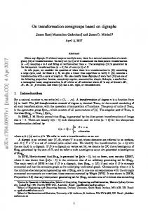
an example how it derives backward transformation functions from view functions that manipulate arbitrary algebraic data structures, including trees. Figure 1 shows the architecture of our bidirectionalization system. The input to our system is a view function. The output consists of a backward transformation function and a checker that validates changes in the view. A change in the view is said to be valid if it can be reflected back to the source by the backward transformation function. The core part is the bidirectional transformation engine mapping from the input to the output. 3.1

transformations, tupling and inversion, based on the constant complement approach to bidirectionalization (Section 6). For the example append , our system first automatically derives the following definition for the tupled function append M , append M append c . append M (Nil, y) = ˆ (y, B1 ) append M (Cons(a, x), y) = ˆ (Cons(a, s), B2 (t)) where (s, t) = ˆ append M (x, y) Then, it derives the following inverse of the tupled function. −1

(append M ) (y, B1 ) = ˆ (Nil, y) −1 (append M ) (Cons(a, s), B2 (t)) = ˆ (Cons(a, x), y) −1 where (x, y) = ˆ (append M ) (s, t)

View Function

Views are generated by application of view functions to sources. View functions are defined in a compositional way like f = (f1 ◦ f2 ) × map f3 . More precisely, a view function is a combination of primitive view functions and the gluing combinators, which were explained in Section 2.4.2. Each primitive function is in the affine, treeless form defined by a constructor-based first-order functional language with pattern matching (Section 4). The patterns and constructors in the language make it easy to code primitive view functions from one algebraic data structure to another. As a simple example, consider generation of a view of a list from two lists by appending them together. This view function can be defined in our language as follows. append (Nil, y) = ˆ y append (Cons(a, x), y) = ˆ Cons(a, append (x, y)) It decomposes the data by pattern matching and constructs new data by data constructors.

Finally, it applies Equation (UPD) in Section 2.4.1 and produces the following backward transformation function. −1

updhappend,append c i (s, v) = ˆ (append M )

To see what the derived backward transformation function actually is, let us rename updhappend,append c i to append B . Applying the fusion transformation (Wadler 1990) can yield the following definition. append B ((Nil, y), v) = ˆ (Nil, v) append B ((Cons(a, x), y), Cons(b, v)) = ˆ (Cons(b, s), t) where (s, t) = ˆ append B ((x, y), v) That is, append B is such a function, accepting the original source (x, y) and a new view v and returning a new source (x0 , y 0 ), where x0 is the first n elements of v and y 0 is the rest. Here, n is the length of x. 3.2.3

3.2 Bidirectional Transformation Engine Since our view functions are compositional, our bidirectionalization basically consists of two parts: • bidirectionalizing primitive view functions, and • bidirectionalizing the gluing view functions combinators.

Given that bidirectionalization of combinators has been well studied (Foster et al. 2005; Hu et al. 2004), we will focus on bidirectionalization of primitive view functions, though the whole system should combine the two. 3.2.1

(v, append c (s))

Generating View Update Checker

As seen in the above example, a derived backward transformation function may be partial: function append B is defined only if the length of the updated view is not less than the length of the first list in the original source. Therefore, the backward transformation will fail if an updated view does not fall in its domain. Our system automatically generates from a given view function, together with the original source, a view update checker, represented by a tree automaton, which can check whether an update on the view is valid or not. Section 7 explains in detail how to generate view update checkers, including a generated automaton for the example append in this section.

Deriving View Complement Functions

Our system starts by automatically deriving a small (with respect to the collapsing order in Definition 2) view complement function for a given view function so that tupling the two functions gives an injective function (Section 5). For example, a view complement function automatically derived by our system for append is as follows. append c (Nil, y) = ˆ B1 append c (Cons(a, x), y) = ˆ B2 (append c (x, y)) In this definition, B1 and B2 are data constructors automatically generated by the system. A close look at the definition reveals that the derived view complement function actually computes the length of the first argument. One can easily verify that although append is non-injective, tupling append and append c , append M append c , is injective. 3.2.2 Deriving Backward Transformation Functions by Tupling and Inversion After obtaining the view complement function, our system generates a backward transformation function based on two program

4. View Definition Language In this section, we introduce our language, V DL, for defining view functions. It is a first-order functional programming language that is similar to Wadler’s language for defining basic functions for fusion (Wadler 1990). 4.1

The Language V DL

The syntax and semantics4 of the language is given in Figure 2. A program of our language consists of a set of function definitions, and each function is defined by several rules of the form f (p1 , . . . , pn ) = ˆ e. To simplify our presentation, we assume that there is no overlap among rules of the same function, i.e., no two patterns in the lefthand side overlap. There are two important syntactic restrictions on each rule declaration. 4 Note that V DL has the call-by-value semantics, where values are expressions that consists of only constructor symbols in C.

data structures. For example, the view function for addition of two natural numbers is defined by

Syntax: rule

::=

f (p1 , . . . , pn ) = ˆ e

p

::= |

C(p1 , . . . , pn ) x

constructor pattern variable pattern

e

::= | |

C(e1 , . . . , en ) f (x1 , . . . , xn ) x

constructor application function call variable

where C ∈ C and f ∈ F are of arity n, and x ∈ X . Operational Semantics: (Con)

e1 ⇓ v1 · · · en ⇓ vn C(e1 , . . . , en ) ⇓ C(v1 , . . . , vn )

f (p1 , . . . , pn ) = ˆ e∈R ∃θ, f (p1 θ, . . . , pn θ) = f (v1 , . . . , vn ) eθ ⇓ u (Fun) f (v1 , . . . , vn ) ⇓ u where “eθ” denotes the expression that is obtained by replacing any variable x in e with the value θ(x), and v1 , . . . , vn denotes values: values are expressions that consist only of constructor symbols in C.

Figure 2. View Definition Language

add (Z, y) = ˆ y add (S(x), y) = ˆ S(add (x, y)). As in Haskell, we use a symbol starting with an uppercase letter to denote a constructor and a symbol starting with a lowercase letter to denote a function or a variable. Function add is defined by traversing over one data structure in the source, while the following function, max , for computing the maximum of two natural numbers is defined by simultaneously traversing over two data structures in the source. max (Z, y) = ˆ y max (S(x), Z) = ˆ S(x) max (S(x), S(y)) = ˆ S(max (x, y)) Example 5 (Recursive View Functions on Lists and Trees). Our language can be used to define view functions on various data structures such as lists and trees. As a view function on lists, the function zip for zipping two lists is defined below. zip(Nil, y) = ˆ Nil zip(Cons(a, x), Nil) = ˆ Nil zip(Cons(a, x), Cons(b, y)) = ˆ Cons(Pair(a, b), zip(x, y)) As a view function on trees, the function for flipping a binary tree is defined below. flip(Leaf) = ˆ Leaf flip(Node(n, l, r)) = ˆ Node(n, flip(r), flip(l))

• The expression, e, of a rule is in a treeless form (Wadler 1990),

i.e., a function call, which may appear inside a constructor application but never appears inside another function call. It can be seen in Figure 2 that each argument to a function call is a variable instead of an expression. This restriction ensures no intermediate data structure in e. • Variable occurrences in a rule are affine, i.e., every variable in

the left-hand side of a rule occurs at most once in the corresponding right-hand side. This restriction ensures that there is no duplication of data. These two syntactic restrictions play an important role in our automatic bidirectionalization framework, simplifying the generation of a view complement function from a view function written in V DL. Though restricted, this language is sufficiently powerful to describe many interesting view functions. It is not difficult to see that the view functions we have seen so far, such as students, mapfst, and append , can be coded in V DL with slight syntactic modification. In the following, we give more examples of view functions in V DL. Example 1 (Identity View Function). The simplest view function is the identity function, which creates a view that is the same as its source. It can be defined in V DL as follows. id (x) = ˆ x Example 2 (Projection View Functions). The projection view functions are useful for selecting a component from the source. They can be defined in V DL as follows. fst(x, y) = ˆ x snd (x, y) = ˆ y Example 3 (Constant View Functions). A constant view function is useful for creating a view that is independent of its source. An example of the constant view function is defined in V DL as follows. nil (x) = ˆ Nil Example 4 (Recursive View Functions on Natural Numbers). Many view functions are defined recursively by traversing over

4.2

Notations for Manipulating Programs in V DL

In the rest of this paper, we will discuss several program transformations and prove important properties for them. To do this, we give a more formal definition of our programs in V DL, and prepare some notations and functions for later program manipulation. Formally, a program P in our language V DL is a 4-tuple (R, F, C, X ) where • R is a set of rules (see Figure 2), • F is a set of function symbols with associated arities, • C is a set of constructor symbols with associated arities, and • X is a set of variables

such that all sets are pairwise disjoint. We call an expression generated only by constructor symbols in C a value or a tree value and use TC to denote the set of all values. A substitution is a mapping θ : X → TC that assigns to a variable a value. We denote by eθ an expression obtained by replacing each variable x in e with a tree θ(x). As discussed before, we do not allow rule overlapping in R. Formally, R is non-overlapping if for any two distinct rules f (p1 , . . . , pn ) = ˆ e ˆ e0 f (p01 , . . . , p0n ) = there is no substitution θ satisfying (p1 , . . . , pn )θ = (p01 , . . . , p0n )θ. → We sometimes use vector notations − e to denote sequence e1 , . . . , en when the length of sequence n is not concerned. For → example, a rule f (p1 , . . . , pn ) = ˆ e is denoted as f (− p)= ˆ e. For a rule r, we write Vars(r) to denote the set of all variables occurring in r, UsedVars(r) the set of all variables occurring in the right-hand side of r, and LostVars(r) = Vars(r) \ UsedVars(r). To prove the properties of programs, we sometimes need to distinguish function symbols from their meanings. We denote the semantics of f by [[f ]]P . Under the operational semantics of V DL, shown in Figure 2, a program P yields a partial function [[f ]]P :

(TC × · · · × TC ) → TC for each function symbol f ∈ F:  v if f (v1 , . . . , vn ) ⇓ v, [[f ]]P (v1 , . . . , vn ) = ⊥ otherwise. Note that when it is clear from the context, [[f ]]P is sometimes simply written as [[f ]] or even f . We add two semantic restrictions to V DL to avoid pathological situations in the proofs of the properties of programs written in V DL. First, a set of constructors C contains at least two constructors and one is zero-arity. Second, V DL does not contain functions that are undefined everywhere. For example, the following function f is undefined everywhere. f (x) = ˆ f (x)

→ where {− y } = LostVars(r) and Br is a fresh constructor, and f c , f1 c , . . . , fn c 6∈ F are function symbols corresponding to f, f1 , . . . , fn respectively. 2. Create a program as follows. P c = ({rc | r ∈ R}, {f c | f ∈ F}, {Br | r ∈ R} ∪ C, X ).2 Theorem 2 (Soundness of ALG c ). Let P = (R, F , C, X ) be a program and P c = (Rc , F c , C c , X c ) the derived program by ALG c . Then, for every function symbol f ∈ F, [[f c ]] is a complement function of [[f ]]. Note that by ALG c , a function is defined if and only if its com→ → plement function is defined, i.e., f (− v ) ↓ if and only if f c (− v ) ↓. Example 6. Consider function fst defined by

5. Deriving View Complement Functions We shall develop algorithms for derivation of view complement functions from view functions so that tupling them gives an injective function. Compared to the algorithms in Cosmadakis and Papadimitriou (1984), Laurent et al. (2001) and Lechtenb¨orger and Vossen (2003), our algorithms are capable of dealing with functions on tree data structures. We start with a direct algorithm, and then improve it with a minimizing procedure with injectivity and range analysis. 5.1 A Direct Solution For a given view function f : S → V , to derive its complement function g : S → V 0 , we should be clear about where the noninjectivity of f comes from. Recall that a complement function g of f is a function that makes the tupled function (f M g) : S → (V × V 0 ) injective. So, if f is injective, its complement function g can be an arbitrary function from S to V 0 (of course, updatability of the backward transformation depends on which g to choose). If f is non-injective, g should return different values for any distinct arguments x, y ∈ S such that f (x) = f (y). Syntactically, there are basically two possible cases for a view function to be non-injective: 1. Some variables on the left-hand side of a rule disappear in the corresponding right-hand side. For example, function fst(x, y) = ˆ x is non-injective. 2. The ranges of two right-hand sides of a view function overlap. For example, the following f is obviously non-injective: f (A) = ˆ A

f (B) = ˆ A.

Using this observation, we give an algorithm to derive a complement function of a view function. Below, we use the context notation. A context K is a tree value containing special holes 21 , . . . , 2n and we denote by K[e1 , . . . , en ] an expression obtained by replacing 2i with ei for each i in {1, . . . , n}. Any expression in treeless form can always be separated as a context, function calls and variables as →), . . . , f (− → − → K[f1 (− x 1 n xn ), x ]. Algorithm 1 (Derivation of Complement Function: ALG c ). Input: A program P = (R, F, C, X ) for view functions. Output: A program P c for view complement functions. Procedure: 1. For each rule r ∈ R → →), . . . , f (− → − → r = f (− p)= ˆ K[f1 (− x 1 n xn ), x ] construct a rule → − → →), . . . , f c (− − x r = f (→ p)= ˆ Br (f1c (− 1 n xn ), y ) c

c

fst(x, y) = ˆ x. In this definition, the second argument, y, is discarded. Algorithm ALG c derives the rule fst c (x, y) = ˆ B1 (y). Here, B1 is the newly-introduced constructor for the first rule. Later, we use the constructor Bi for the ith rule. That is, function fst c “complements” lost value “y” in the definition of fst. Example 7. Consider the function add defined in Example 4. In this definition, all variables are preserved from the left-hand side to the right-hand side of each rule. Algorithm ALG c derives the following two rules. add c (Z, y) = ˆ B1 add c (S(x), y) = ˆ B2 (add c (x, y)) This function add c actually returns the information of the first argument. Example 8. Consider the function max defined in Example 4. Algorithm ALG c derives the following three rules. max c (Z, y) = ˆ B1 max c (S(x), Z) = ˆ B2 max c (S(x), S(y)) = ˆ B3 (max c (x, y)) This complement function is basically equivalent, with respect to the collapsing order, to the following function, minle, which returns the minimum of arguments and a boolean value indicating whether the first argument is “less than or equal” to the second.  (x, 1) if x ≤ y minle(x, y) = (y, 0) if x > y In general, there can be infinitely many complement functions for a given view function. Ideally, we want to obtain a complement function that is minimal with respect to the collapsing order. The function, fst c , derived by ALG c is a minimal complement of fst, but a complement function derived by ALG c is not always a minimal one. Next we will consider how to obtain smaller complement functions. 5.2

Making it Smaller

Algorithm ALG c does not always return a minimal complement function. For example, consider the following function not. not(True) = ˆ False

not(False) = ˆ True

Since the function not is injective, a minimal complement of this function can be any constant function. But Algorithm ALG c derives the rules not c (True) = ˆ B1

not c (False) = ˆ B2

which is obviously not a constant function.

To derive smaller complement functions, we improve Algorithm ALG c by analyzing injectivity of function, and calculating ranges of the right-hand-side expressions. These two kinds of analysis are useful to minimize complement functions for the following reasons: 1. If the input function is recognized to be injective, we should return a constant function. This requires determination of the injectivity of a function. Fortunately, this is decidable in V DL. In the next subsection, we present an algorithm to determine injectivity. 2. Let e be an expression that may contain free variables. By the range of an expression e, we mean the set of evaluated values of all possible ground instances of e, i.e., the set defined by Range(e) = {v | ∃θ : X → TC , eθ ⇓ v}.

5.2.2

For every expression occurring in a program, we can construct an automaton that accepts exactly the trees in the range of the expression. Our idea was based on the existing result that the image of a linear tree transducer is a regular tree language (Engelfriet 1975). Let P = (R, F , C, X ) be a program and E be a set of expressions occurring in R. For an expression e ∈ E, we construct a nondeterministic (bottom-up) finite tree automaton Ae over C. This automaton is a tuple (Q, C, {qe }, ∆) with a set of states Q, a set of constructors C, the unique final state qe , and a set of transition rules ∆ where • Q = {qf | f ∈ F} ∪ {qe0 | e0 ∈ E} ∪ {q∗ } • ∆ consists of

q∗ → qe0 with e0 = x ∈ E and x ∈ X ,

Suppose that we have two rules f (C1 (x)) = ˆ e1

3. In addition to the above, the range analysis is helpful to remove unnecessary unary constructors. For example, let f be a view function and f c be its complement function. f (C1 (x)) = ˆ D1 (f (x)) c

qf → qe0 with e0 = f (. . . ) ∈ E and f ∈ F,

f (C2 (x)) = ˆ e2 .

If the ranges of e1 and e2 do not overlap, f c (C1 (x)) and f c (C2 (x)) can be safely collapsed to the same value for some input, and hence [[f c ]] becomes smaller. In Section 5.2.2 we present an algorithm to calculate the range of an expression by using a tree automaton.

c

Range Analysis

f (C2 ) = ˆ D2

f (C3 ) = ˆ D2

c

f (C1 (x)) = ˆ B1 (f (x)) f (C2 ) = ˆ B2 f c (C3 ) = ˆ B3 The unary constructor, B1 , can be removed if the ranges of D1 (f (x)) and D2 do not overlap. This is because the ranges of right-hand-side expressions of tupled function (f M f c ) do not overlap if for any two rules r1 , r2 of f either the ranges of right-hand-side expressions of r1 , r2 or r1 c , r2 c do not overlap. The obtained complement function defined as f c (C1 (x)) = ˆ f c (x) f c (C2 ) = ˆ B2

f c (C3 ) = ˆ B3

is smaller than the original complement function. 5.2.1 Injectivity Analysis We present an algorithm that determines the injectivity of a function. The algorithm consists of three major steps. In every step, the algorithm marks functions if they are non-injective and otherwise proceeds to other steps. All functions unmarked at the end are injective. Algorithm 2 (Injectivity Checking: ALG i ). Input: A program P = (R, F, C, X ) for view functions. Output: For each function f ∈ F , “f is injective” or “f is noninjective”. Procedure: 1. Mark those functions that have a rule discarding variables. 2. Mark those functions whose ranges of right-hand sides of two distinct rules overlap. 3. Repeat Mark those functions that call marked functions. Until no marking can be done. 4. Return “f is non-injective” if f is marked, otherwise return “f is injective”. 2 Theorem 3 (Soundness and Completeness of ALG i ). For every function symbol f ∈ F , ALG i returns “f is injective” if and only if [[f ]] is an injective function.

C(qe1 , . . . , qen ) → qe0 with e0 = C(e1 , . . . , en ) ∈ E, qe0 → qf for f (. . . ) = ˆ e0 ∈ R and C(q∗ , . . . , q∗ ) → q∗ with C ∈ C. The following lemma states that automaton Ae exactly accepts the trees in the range of e. Lemma 1 (The Range of Expressions). Let P = (R, F , C, X ) be a program. For each expression e occurring in P , a tree t is in the range of e if and only if the tree automaton, Ae , accepts t. The ranges of two expressions e and e0 overlap if and only if the language accepted by the intersection of two tree automata Ae and Ae0 is not empty. Since finite tree automata are closed under intersection and the emptiness of a finite tree automaton is decidable (Comon et al. 1997), we have the following corollary. Corollary 1. For a program P = (R, F, C, X ), whether the ranges of two expressions in R overlap or not is decidable. 5.2.3

Deriving Smaller Complement Functions

With injectivity and range analysis, we can improve Algorithm ALG c and derive smaller complement functions. We change three parts in the original algorithm. First, we remove f c (. . . ) for every injective function f from arguments of B in ALG c in the construction of the complement, because a complement function of any injective function is a constant function and can be ignored. Second, we use the same constructor for those rules of f c when the ranges of the right-hand-side expressions of these rules do not overlap. Third, we remove a unary constructor from a rule for f c , if the range of the right-hand-side expression of the corresponding rule of f does not overlap with the ranges of other rules of f . As a preprocessing step, we calculate a partition of R = R1 ] · · · ] Rk such that for each rule subset Ri the following hold. • For all r, r 0 ∈ Ri , r and r 0 define the same function. • For all r, r 0 ∈ Ri , the sum of non-injective functions and lost

variables in both rules are the same. • For all r, r 0 ∈ Ri , the ranges of the right-hand-side expressions

of r and r0 do not overlap.

Algorithm 3 (Improvement of ALG c : ALG sc ). Input: A program P = (R, F , C, X ) for view functions and a partition of R = R1 ] · · · ] Rk . Output: A program P c for view complement functions.

which is a minimal complement function of mapnot with respect to the collapsing order. It is worth remarking that Algorithm ALG sc will derive constant functions for injective functions if a partition of R is R = Rf1 ] · · · ] Rfn where Rfi is the set of all rules for fi . The existence of such a partition is easily checked by the range analysis.

Procedure: For each rule r for defining f ∈ F: → →), . . . , f (− → − → r = f (− p)= ˆ K[f1 (− x 1 n xn ), x ] ∈ Rj do the following: 1. Construct a rule

−→ → → c − → 0 c c y) (x0m ), − = f c (− p)= ˆ Bk (f10 (x01 ), . . . , fm rpre −→ − →0 0 0 0 where the function calls f1 (x1 ), . . . , fm (xm ) are obtained →), . . . , f (− → from f1 (− x 1 n xn ) all injective function calls removed, → and {− y } = LostVars(r).

c is in the form of 2. If rpre

→ c − − f (→ p)= ˆ Bj (f 0 ( x0 )) c

and the right-hand-side expression of r does not overlap with the right-hand-side expression of any other rule r0 for f ∈ F , construct a rule → c − → rc = f c (− p)= ˆ f 0 ( x0 ), otherwise, construct a rule c . rc = rpre

3. Create a program as follows. P = ({r | r ∈ R}, {f | f ∈ F}, {Bj | Rj }, X ) c

c

c

2

Theorem 4 (Soundness of ALG sc ). Let P = (R, F, C, X ) be a program and P c = (Rc , F c , C c , X c ) the derived program by ALG sc . Then, for every function symbol f ∈ F , [[f c ]] is a complement function of [[f ]]. Example 9 (Role of Rule Partition). Consider the function, f , defined by r1 = f (A1 ) = ˆ C1 r2 = f (A2 ) = ˆ C2 r3 = f (A3 ) = ˆ C1 and suppose that R = {r1 , r2 } ] {r3 }. Then, Algorithm ALG sc returns the following complement function. f c (A1 ) = ˆ B1 f c (A2 ) = ˆ B1 f c (A3 ) = ˆ B2

f c (A1 ) = ˆ B1 f c (A2 ) = ˆ B2 f c (A3 ) = ˆ B2 So different rule partitions can lead to different complement functions. This is why we separate rule partitions from Algorithm ALG sc . Example 10 (Complements of Injective Functions). Consider the function, mapnot, defined as follows. = ˆ = ˆ = ˆ = ˆ

Cons(not(a), mapnot(x)) Nil False True

In contrast with mapfst defined above, mapnot is injective. With injective analysis we know that mapnot and not are injective functions, so ALG sc returns the following complement functions mapnot c (Cons(a, x)) mapnot c (Nil) not c (True) not c (False)

zip c (Nil, y) = ˆ B1 (y) zip c (Cons(a, x), Nil) = ˆ B2 (a, x) zip c (Cons(a, x), Cons(b, y)) = ˆ zip c (x, y) which is a minimal complement function of zip c . Note that ALG sc has removed the constructor from the third rule, compared to the old algorithm, ALG c . The complement functions obtained by ALG sc have two good characteristics. First, they have the same form as view functions, which makes the later tupling step and the inversion step easy. Second, as will be seen later, the updatability of backward transformation functions with these complement functions is easy to understand.

6. Generating Backward Transformation Functions After obtaining a view complement function f c : S → V 0 for a given view function f : S → V , we get the following backward transformation according to Equation (UPD). ρ(s, v) = (f M f c )−1 (v, f c (s)) That is, a backward transformation function can be derived if the tupled function, (f M f c ), and its inverse (f M f c )−1 can be effectively derived. The point is how to calculate an inverse program. Although this is generally difficult, now we need merely to treat the tupled function of the form (f M f c ). Thanks to the correspondence between the rules of f and f c , we can obtain a program of (f M f c ) which is in a good form for this inversion. In the following, we show how tupling and inversion can be done automatically. 6.1

However, if R = {r1 } ] {r2 , r3 }, ALG sc will return another complement function.

mapnot(Cons(a, x)) mapnot(Nil) not(True) not(False)

Example 11 (Removing Constructors). Consider the function zip in Example 5. Algorithm ALG sc returns

= ˆ = ˆ = ˆ = ˆ

B1 B1 B2 B2

Calculation of Program of (f M f c )

A program for tupled function (f M f c ) can be straightforwardly calculated because the rules of f and the corresponding f c have the same patterns and the same form of recursive calls in the right-hand sides. However, we cannot directly describe the tupled function in the treeless form because of the tuple structure, which needs to be treated specially. We extend language V DL with “where-clauses” and tuples: rule ::= · · · | f (p1 , . . . , pn ) = ˆ (e1 , . . . , em ) where (x1 , . . . , xk ) = ˆ g(y1 , . . . , ym ) ... 0 ˆ g 0 (y10 , . . . , ym (x01 , . . . , x0k0 ) = 0) where e1 , . . . , en do not include any function calls, i.e., they have the same forms as patterns, and all variables appear on the left-hand sides of the where-clause are different from those on the righthand sides. The two restrictions above are the treeless condition of tupled functions. Additionally, this new form of rules must satisfy the affine condition. That is, all variables used at most once (actually, all variables are used exactly once in tupled functions). The operational semantics is straightforwardly extended. Note that this extension is behind the scene of the view definition users; it is only used internally during bidirectionalization transformation.

Algorithm 4 (Tupling). Input: A where-free program P . Output: A program P M for tupled functions. Procedure:

a domain analysis similar to the range analysis discussed before, when the inverse program is executed. An example of inversion is given in Section 8.

1. Let P c be the program derived from P by ALG sc . 2. For each non-injective function f , and for each rule r of f in P do (a) Let rc be the corresponding rule for r in P c . (b) Structure r and rc in the following forms → → − − → r = f (− p)= ˆ K[ t , − u,→ x] → − − → → c c − 0 0 r = f (p)= ˆ K [ t , x0 ] where − → → • t : non-injective function calls f1 (− y1 ), . . . , fn (− y→ n ), − →0 → − →), • t : function calls of the forms f1 c (− y1 ), . . . , fn c (y n → → • − u : injective function calls g1 (− z1 ), . . . , gm (− z→ m ). (c) Prepare fresh variables ti , t0i , uj for i ∈ {1, . . . , n}, j ∈ {1, . . . , m}. (d) Construct the rule, rM , as follows: → − − → → → − − → rM = f M (− p)= ˆ (K[ t , − u ,→ x ], K 0 [ t0 , x0 ]) → ˆ fi M (− where {(ti , t0i ) = yi )}i∈{1,...,n} → − {u = ˆ g ( z )} j

j

j

j∈{1,...,m}

3. For each injective function g, and for each rule r of g in P , construct the rule, r0 , as follows in the similar way: → → → r0 = g(− p)= ˆ K[− u ,− x] → where {uj = ˆ gj (− zj )}j∈{1,...,m}

4. Gather all rM and r0 to form P M .

2

This algorithm correctly gives a program of tupled functions, → − → − i.e., [[f M ]]( t ) = ([[f ]] M [[f c ]])( t ). An example is given in Section 8. 6.2 Calculation of Program of (f M f c )−1 Next, we calculate an inverse program for (f M f c )−1 from the program of (f Mf c ). The basic idea is to swap the left-hand side and the right-hand side of each rule and to apply inversion recursively. Algorithm 5 (Inversion of Tupled Functions). Input: A program P M = (R, F , C, X ) for tupled functions. Output: A program ` ˘ ¯ ´ −1 (P M ) = R−1 , f −1 | f ∈ F , C, X for tupled functions. Procedure: For each rule r in R → → → ˆ fi (− yi )}i∈{1,...,n} r = f (− p)= ˆ (− e ) where {(ti , t0i ) = → {uj = ˆ gj (− zj )}j∈{1,...,m} construct the rule r−1 in R−1 as follows. → → → r−1 = f −1 (− e)= ˆ (− p ) where {(− yi ) = ˆ fi−1 (ti , t0i )}i∈{1,...,n} → − {( zj ) = ˆ gj−1 (uj )}j∈{1,...,m} 2 −1

Theorem 5 (Correctness). Let P be a program, and (P M ) the generated program. Then, (u1 , u2 ) = [[f M ]]P M (t1 , . . . , tn ) implies (t1 , . . . , tn ) = [[(f M )−1 ]](P M )−1 (u1 , u2 ). Note that the obtained inverse program may be nondeterministic. However, since the original function to be inversed is injective in our framework, it is possible to uniquely determine a rule with

7. Generating View Update Checker A view update checker is designed to decide whether or not an update on views is valid without execution of the backward transformation. An update on views is said to be valid if it can be successfully reflected to the source by the derived backward transformation function. Recall that in our framework, a backward transformation is given by updhf,f c i (s, v) = ˆ (f M f c )−1 (v, f c (s)). This means that, for a view function f and the original source, s, we can check whether or not a view update is valid by confirming whether (v, f c (s)) is in the range of (f M f c ), where v is an updated view. We define below a nondeterministic (bottom-up) tree automaton for validating view updates. The tree automaton has three kinds of states: state q∗ is reached by any view, state qf is reached by a view in the range of f , and state qft M is reached by a view v such that (v, t) is in the range of f M . Therefore, when the final state is a state qft0M , the tree automaton exactly accepts a view v such that (v, t0 ) −1 is in the range of f M (i.e., (v, t0 ) is in the domain of (f M ) ). Definition 3 (View Update Checker). Let P be a program, P c be a complement program derived by our algorithm, t0 be a complement view, and P M = (RM , F M , C M , X M ) be a tupled program of P and P c . A view updating checker is defined as a tree automaton AU = (Q, C M , {qft0 }, ∆) where • Q = {q∗ }∪{qf | f ∈ F}∪{qft M | f M ∈ F M , t is a subtree of t0 } • ∆ consists of the following transition rules:

C(q∗ , . . . , q∗ ) → q∗ with C ∈ C, → − → − → ˆ K[− − K[− q→ t ,→ x ] ∈ R and f 0 , q∗ ] → qf with f ( p ) = → 0 − ti = fi ( e ), and −−→ 0 → − t00 K[qft 0θM , − q→ g 0 , q∗ ] → qf M with 2 3 → − − → → → − − → f M (− p)= ˆ (K[ t , − u,→ x ], K 0 [ t0 , x0 ]) M M → 4 where {(ti , t0i ) = ˆ fi0 (− yi )}i∈{1,...,n} 5 ∈ R → 0 − {uj = ˆ gj ( zj )}j∈{1,...,m} → − − → 00 where t is a subtree of t0 and t00 = K 0 [ t0 , x0 ]θ. Theorem 6 (Validity of View Update Checker). A view updating checking tree automaton AU = (Q, C M , {qft0M }, ∆) in Definition 3 exactly accepts view v such that (v, t0 ) is in the range of f M . We show examples of automatically generated view update checkers for some view functions. Note that the view update checking automata below have been reduced where unnecessary states have been removed. Example 12. Consider function append and its complement function in Section 3. When the initial source is (s1 , s2 ) = (Cons(True, Cons(False, Nil)), Nil), the view is append (s1 , s2 ) = Cons(True, Cons(False, Nil)) and the complement view is append c (s1 , s2 ) = B2 (B2 (B1 )). Then, the view update checker generated by our system is the B2 (B2 (B1 )) }, ∆) where automaton A = (Q, C, {qappend M B2 (B1 ) B2 (B2 (B1 )) B1 • Q = {q∗ , qappend , qappend M , qappend M } and M • ∆ consists of the transition rules of

t → q∗ where t ∈ {True, False, Nil}, Cons(q∗ , q∗ ) → q∗ , B2 (B1 ) B2 (B2 (B1 )) Cons(q∗ , qappend , M ) → qappend M

B (B )

B1 2 1 Cons(q∗ , qappend M ) → qappend M , and

q∗ →

and inversion of this tupled function yields the following result. −1

B1 qappend M.

In fact, this automaton only accepts lists that are 2 or longer, which means one can only update the view of lists in such a way that its length is not less than 2. Example 13. Consider the function, filter , defined as filter (Nil) filter (Cons(A1 , x)) filter (Cons(A2 , x)) filter (Cons(A3 , x))

= ˆ = ˆ = ˆ = ˆ

Nil Cons(A1 , filter (x)) Cons(A2 , filter (x)) filter (x)

and the complement function derived by our algorithm as follows. c

filter (Nil) filter c (Cons(A1 , x)) filter c (Cons(A2 , x)) filter c (Cons(A3 , x))

= ˆ = ˆ = ˆ = ˆ

B1 B2 (filter c (x)) B2 (filter c (x)) B3 (filter c (x))

When the initial source is s = Cons(A2 , Cons(A3 , Cons(A1 , Nil))), the view is filter (s) = Cons(A2 , Cons(A1 , Nil)) and the complement view is filter c (s) = B2 (B3 (B2 (B1 ))). Then, the view update checker derived by our system is automaB2 (B3 (B2 (B1 ))) ton A = (Q, C, {qfilter }, ∆) where M B2 (B1 ) B3 (B2 (B1 )) B2 (B3 (B2 (B1 ))) B1 • Q = {qfilter , qfilter , qfilter M , qfilter M } M M • ∆ consists of transition rules B (B (B1 ))

3 2 Cons(t, qfilter M

B (B (B2 (B1 )))

2 3 ) → qfilter M

where t ∈ {A1 , A2 },

B (B )

B1 2 1 Cons(t, qfilter M ) → qfilter M where t ∈ {A1 , A2 }, B2 (B1 ) qfilter M

Nil →

→

B3 (B2 (B1 )) , qfilter M

and

B1 qfilter M.

This automaton accepts lists that are 2 long, and each list element is either A1 or A2 .

8. An Example To give a whole picture of how our system works concretely, recall the example in the Introduction. The following view function, students, is the same as that in the Introduction, except that we write Cons for (:) and Nil for [ ]. students(Nil) = ˆ Nil students(Cons(Student(name, grade, major )), ms)) = ˆ Cons(Student(name, grade, major ), students(ms)) students(Cons(Prof(name, position, major )), ms)) = ˆ students(ms) The function, students, extracts all student members from a member list. This behavior of students is similar to the function, filter . The derived complement function by our algorithm is as follows. students c (Nil) = ˆ B1 students c (Cons(Student(name, grade, major )), ms)) = ˆ B2 (students c (ms)) students c (Cons(Prof(name, position, major )), ms)) = ˆ B3 (name, position, major , students c (ms)) Tupling the two functions students and students c gives students M (Nil) = ˆ (Nil, B1 ) students M (Cons(Student(name, grade, major ), ms)) = ˆ (Cons(Student(name, grade, major ), x), B2 (y)) where (x, y) = ˆ students M (ms) M students (Cons(Prof(name, position, major ), ms)) = ˆ (x, B3 (name, position, major , y)) where (x, y) = ˆ students M (ms),

(students M ) (Nil, B1 ) = ˆ Nil −1 (students M ) (Cons(Students(n, g, m), x), B2 (y)) = ˆ Cons(Student(n, g, m), ms) −1 where ms = ˆ (students M ) (x, y) M −1 (students ) (x, B3 (n, p, m, y)) = ˆ Cons(Prof(n, p, m), ms) −1 where ms = ˆ (students M ) (x, y) Then, a backward transformation ρ = updhstudents,students c i can be derived (after some fusion transformation) as follows. ρ(Nil, Nil) = Nil ρ(Cons(Student(n, g, m), ms), Cons(Student(n0 , g 0 , m0 ), ss)) = Cons(Student(n0 , g 0 , m0 ), ρ(ms, ss)) ρ(Cons(Prof(n, g, m), ms), ss) = Cons(Prof(n, g, m), ρ(ms, ss)) This is exactly the same function as students B in the Introduction. Now one can freely change the names in the view, and the backward transformation can reflect them to the source. Consider the case where the source s is as follows. s = Cons(Student(X, DC, CS), Cons(Prof(Y, AP, CS), Nil)) Let v be the view generated by the view function, students, on s, i.e., v = Cons((Student(X, DC, CS), Nil). Updating view v to Cons(Student(X, DC, Math), Nil) is acceptable and results in the following source. Cons(Student(X, DC, Math), Cons(Prof(Y, AP, CS), Nil)) However, both inserting and removing elements, e.g., updating the view to Nil, are prohibited. This updatability can be precisely represented by an automaton. Let v1 = B2 (B3 (Y, AP, CS, B1 )) v2 = B3 (Y, AP, CS, B1 ) v3 = B1 , then updatability of v with respect to source s is captured by v1 automaton A = (Q, C, {qstudents }, ∆), where v1 v2 v3 • Q = {qstudents , qstudents , qstudents , q∗ }

• ∆ consists of transition rules

C(q∗ , . . . , q∗ ) → q∗ where C ∈ C, v2 v1 Cons(Student(q∗ , q∗ , q∗ ), qstudents ) → qstudents , v3 v2 qstudents → qstudents , and v3 Nil → qstudents .

Note that the view, Cons((Student(X, DC, CS), Nil), is accepted by the automaton, A, but the view, Nil, is not.

9. Related Work Our work is based on the idea of deriving (relational) complement functions on relational databases, where view functions are expressed in terms of relational algebras. Cosmadakis and Papadimitriou (1984) showed that finding minimal complement functions when views are defined only by projections is NP-Complete. Laurent et al. (2001) proposed an algorithm to compute complement functions when views are defined by projections, selections, and joins. They also discussed the conditions for minimal complement functions. Their algorithm is expensive because it uses the results of NP-Complete sub-problems. Lechtenb¨orger and Vossen (2003) improved on Laurent et al.’s work. They proposed a polynomialtime algorithm for computing complement functions when views are defined by projections, selections, joins, and renaming. Their

algorithm computes smaller complement functions than Laurent et al.’s, and the obtained complement functions are minimal when view functions contain no projection. Our work can be considered an extension of these works such that view functions can be defined on tree-like data structures other than tuples. Moreover, our approach is based on syntactic program transformations, whereas the existing methods focus more on function semantics. Our work was greatly motivated by works on bidirectional transformation on trees. In addition to the work by Foster et al. (2005) that proposed a combinatorial approach to the problem (as discussed in the Introduction), Hu et al. (2004) showed how bidirectional transformation can be used to maintain data dependency in the tree view, which can be seen as an application that develops constraint maintainers on trees (Meertens 1998). Mu et al. (2004) improved the consistency of Hu et al.’s framework by imposing restrictions on updating operators. These frameworks are domainspecific and designed for specific applications. In contrast, our work is more general. Our work is also related to work on updating XML views constructed from relational data. Wang and Rundensteiner (2004) applied the work in Dayal and Bernstein (1982) to XML views over relational data. Braganholo et al. (2004) proposed an algorithm to map updates on XML views to relational data. However, they did not consider the case where the source is XML too, and our method may shed a new light on their problems.

10.

Conclusion

This paper presents a new transformational approach to bidirectionalization that can automatically derive backward transformation programs from view definition programs written in a simple functional language. The new bidirectionalization method is built upon three program transformations: automatic derivation of complement functions, tupling transformation, and inverse transformation. These three transformations are composed together through programs in a treeless and affine form, which simplifies and enables implementation of the transformations and automatic generation of a view update checker. Our approach is different from many existing approaches where only a bidirectional interpreter is derived and execution of the interpreter requires passing the source through all the interpretation steps, our approach does produce a program for backward transformation. This makes it possible to utilize an optimizing compiler for more efficient execution of backward transformation. There are several issues that are worth looking into in the future. First, it would be interesting to see if our view language could be extended with regular patterns and the restriction on variable uses could be relaxed so that more view functions could be defined and backward transformation could be derived. Second, we want to see if our bidirectionalization framework can be adapted to other bidirectional semantics. The bidirectional properties (semantics) used in this paper are known as “closed update semantics” where sources are invisible to the users who want to modify views. There is another useful semantics called “open update semantics” where both the source and the view are visible to users. Third, although the system has been implemented, we would like to test it with more practical applications.

References F. Bancilhon and N. Spyratos. Update semantics of relational views. ACM T. Database Syst., 6(4):557–575, 1981. V. P. Braganholo, S. B. Davidson, and C. A. Heuser. From XML view updates to relational view updates: old solutions to a new problem. In VLDB ’04: International Conference on Very Large Data Bases, pages 276–287, 2004.

H. Comon, M. Dauchet, R. Gilleron, F. Jacquemard, D. Lugiez, S. Tison, and M. Tommasi. Tree automata techniques and applications. http://www.grappa.univ-lille3.fr/tata, 1997. S. S. Cosmadakis and C. H. Papadimitriou. Updates of relational views. J. ACM, 31(4):742–760, 1984. U. Dayal and P. A. Bernstein. On the correct translation of update operations on relational views. ACM T. Database Syst., 7(3):381–416, 1982. J. Engelfriet. Bottom-up and Top-down Tree Transformations — A Comparison. Math. Syst. Theory, 9(3):198–231, 1975. J. N. Foster, M. B. Greenwald, J. T. Moore, B. C. Pierce, and A. Schmitt. Combinators for bi-directional tree transformations: a linguistic approach to the view update problem. In POPL ’05: Proceedings of the 32nd ACM SIGPLAN-SIGACT symposium on Principles of programming languages, pages 233–246, 2005. G. Gottlob, P. Paolini, and R. Zicari. Properties and update semantics of consistent views. ACM T. Database Syst., 13(4):486–524, 1988. S. J. Hegner. Foundations of canonical update support for closed database views. In ICDT ’90: Proceedings of the Third International Conference on Database Theory, pages 422–436, 1990. Z. Hu, S.-C. Mu, and M. Takeichi. A programmable editor for developing structured documents based on bidirectional transformations. In PEPM ’04: Proceedings of the 2004 ACM SIGPLAN symposium on Partial evaluation and semantics-based program manipulation, pages 178–189, 2004. R. L¨ammel. Coupled software transformations (extended abstract). In First International Workshop on Software Evolution Transformations, pages 31–35, 2004. D. Laurent, J. Lechtenb¨orger, N. Spyratos, and G. Vossen. Monotonic complements for independent data warehouses. VLDB J., 10(4):295– 315, 2001. J. Lechtenb¨orger and G. Vossen. On the computation of relational view complements. ACM T. Database Syst., 28(2):175–208, 2003. K. Matsuda, Z. Hu, K. Nakano, M. Hamana, and M. Takeichi. Bidirectionalization transformation based on automatic derivation of view complement function. Technical Report 2007-44, Graduate School of Information Science and Technology, the University of Tokyo, 2007. L. Meertens. Designing constraint maintainers for user interaction. http://www.cwi.nl/~lambert, 1998. S.-C. Mu, Z. Hu, and M. Takeichi. An algebraic approach to bidirectional updating. In APLAS ’04: Second ASIAN Symposium on Programming Languages and Systems, pages 2–18, 2004. P. Wadler. Views: a way for pattern matching to cohabit with data abstraction. In POPL ’87: Proceedings of the 14th ACM SIGACT-SIGPLAN symposium on Principles of programming languages, pages 307–313, 1987. P. Wadler. Deforestation: Transforming programs to eliminate trees. Theor. Comput. Sci., 73(2):231–248, 1990. L. Wang and E. A. Rundensteiner. On the updatability of XML views published over relational data. In ER 2004: International Conference on Conceptual Modeling, pages 795–809, 2004.