Advanced Nonlinear Studies 10 (2010), 597–609
Bifurcation of Limit Cycles from a Polynomial Degenerate Center Adriana Buic˘ a
∗
Department of Applied Mathematics, Babe¸s-Bolyai University RO-400084 Cluj-Napoca, Romania e-mail:
[email protected]
Jaume Gin´ e
∗
Departament de Matem` atica, Universitat de Lleida Av. Jaume II, 69, 25001 Lleida, Catalonia, Spain e-mail:
[email protected]
Jaume Llibre
†
Departament de Matem` atiques, Universitat Aut` onoma de Barcelona 08193 Bellaterra, Barcelona, Catalonia, Spain e-mail:
[email protected] Received 23 July 2009 Communicated by Rafael Ortega
Abstract Using Melnikov functions at any order, we provide upper bounds for the maximum number of limit cycles bifurcating from the period annulus of the degenerate center x˙ = −y((x2 + y 2 )/2)m and y˙ = x((x2 + y 2 )/2)m with m ≥ 1, when we perturb it inside the whole class of polynomial vector fields of degree n. The positive integers m and n are arbitrary. As far as we know there is only one paper that provide a similar result working with Melnikov functions at any order and perturbing the linear center x˙ = −y, y˙ = x. ∗ The authors are partially supported by a MCYT/FEDER grant number MTM2008-00694 and by a CIRIT grant number 2009SGR 381 † The author is partially supported by a MCYT/FEDER grant number MTM2008-03437 and by a CIRIT grant number 2009SGR 410
597
598
A. Buic˘ a, J. Gin´e, J. Llibre
1991 Mathematics Subject Classification. Primary 34C05, 34C07. Key words. limit cycles, degenerate center, polynomial differential system
1
Introduction and statement of the main results
Probably the main problem in the qualitative theory of real planar differential systems is the determination of its limit cycles. A limit cycle of a planar differential system was defined by Poincar´e [12], as a periodic orbit of the differential system isolated in the set of all periodic orbits. At the end of the 1920s van der Pol [13], Li´enard [11] and Andronov [1] proved that a periodic orbit of a self–sustained oscillation occurring in a vacuum tube circuit was a limit cycle as considered by Poincar´e. After these works the non-existence, existence, uniqueness and other properties of limit cycles were studied extensively by mathematicians and physicists, and more recently also by chemists, biologists, economists, etc. (see for instance the books [4, 17]). During 1881–1886 Poincar´e defined the notion of a center of a real planar differential system, as an isolated singular point having a neighborhood such that all the orbits of this neighborhood are periodic with the unique exception of the singular point. Then one way to produce limit cycles is by perturbing a system which has a center, in such a way that limit cycles bifurcate in the perturbed system from some of the periodic orbits of the unperturbed one [14]. This procedure is effective if one knows the first integral of the unperturbed system, sometime to determine it is a difficult problem, see for instance [5, 6, 8]. In this paper we consider the polynomial differential system ( 2 )m ( 2 )m x + y2 x + y2 x˙ = −y , y˙ = x , (1.1) 2 2 of degree 2m + 1 having a degenerate center at the origin when m is a positive integer, and we perturb it inside the class of polynomial differential systems of degree max{2m + 1, n} given by ( 2 )m ∑ ( 2 )m ∑ ∞ ∞ x + y2 x + y2 k x˙ = −y + ε fk (x, y), y˙ = x + εk gk (x, y), (1.2) 2 2 k=1
k=1
where fk and gk are polynomials of degree n for k = 1, 2, . . ., and ε > 0 is a sufficiently small parameter. Clearly H = (x2 + y 2 )/2 is a first integral of the unperturbed system (1.1). Note that H can take values in [0, ∞), and that for every h ∈ (0, ∞) the circle H = h corresponds to a periodic orbit of the unperturbed system (1.1). Consider the positive x-half-axis Γ parameterized by h, i.e. the point (x, 0) has the h value x2 /2. For ε > 0 sufficiently small we define Pε : Γ → Γ as h 7→ Pε (h), where Pε (h) is the first intersection with Γ in forward time of the orbit of system (1.2) through the point (x, 0). In other words Pε (h) is the so called first return map of the perturbed system (1.2) in terms of h and ε. Of course P0 (h) is the identity map.
Bifurcation of limit cycles from a polynomial degenerate center
599
The displacement function d(h, ε) = Pε (h) − h has the following representation in power series in ε d(h, ε) = εM1 (h) + ε2 M2 (h) + ε3 M3 (h) + · · · ,
(1.3)
which is convergent for sufficiently small ε, and where the coefficients Mk (h) are called the Melnikov functions defined for h ≥ 0. Clearly each simple zero h0 ∈ (0, ∞) of the first non-vanishing coefficient in (1.3) corresponds to a limit cycle of (1.2). For studying the limit cycles of a perturbed differential system which bifurcate from the periodic orbits of a center of an unperturbed differential system, there are many papers which study the simple zeros of M1 (h), assuming that it is the first non-vanishing Melnikov function; there are few papers which study the simple zeros of M2 (h), assuming that it is the first non-vanishing Melnikov function; and there are very few papers which study the simple zeros of M3 (h), assuming that it is the first non-vanishing Melnikov function. As far as we know Iliev in [9] was the first in studying the simple zeros of Mk (h), assuming that it is the first non-vanishing Melnikov function, for an arbitrary k. Since such study perturbing a general center is not possible to do due to the extreme difficulty of the computations that it needs, Iliev does it for the easiest center, the linear one, i.e. the center of system (1.1) with m = 0. Here following the ideas of Iliev we shall extend his results to any m ≥ 1. The main result of this paper is the following. Theorem 1.1 Assume that m in system (1.2) is a positive integer. Suppose that the first Melnikov function in (1.3) which is not identically zero is Mk (h) for some k ≥ 1. All the zeros of the function Mk (h) will be counted with their multiplicities. Then the following statements hold. (a) M1 (h) has at most [ 12 (n − 1)] positive zeros. (b) If n ≥ 2m + 1 and k ≥ 2, then the degree of system (1.2) is n and Mk (h) has at most [ 21 k(n − 1)] + k − 2 positive zeros. (c) If n ≤ 2m and k ≥ 2, then the degree of system (1.2) is 2m + 1 and Mk (h) has at most [ 12 (n − 1)] + (k − 1)(m + 1) − 1 positive zeros. (d) For n ≥ 2 the upper bounds given above for k = 1, and for k = 2 and n ≥ m are reached for convenient perturbations f and g in (1.2). Moreover for k = 2 and n ≤ m − 1 the upper bound given in (c) can be reduced to [ 12 (n − 1)] + n, and this new upper bound is reached. (e) For n = 1 the number of positive zeros of Mk (h) is always zero. (f ) For k > 2 the upper bounds given in statements (b) and (c) are usually not reached. More precisely, the numbers between parentheses in Tables 1 and 2 are the maximum reached upper bounds, which are smaller than the upper bounds given in (b) and (c).
600
A. Buic˘ a, J. Gin´e, J. Llibre
Here and below [r] denotes the entire part of r ∈ R. The first three statements of Theorem 1 give an upper bound for the number of limit cycles emerging from the period annulus of the center of the unperturbed system. In [10] Iliev studied the case m = 0 (i.e. the bifurcations of limit cycles from the harmonic oscillator), and proved that the function Mk (h) has at most [ 12 k(n − 1)] zeros, counting their multiplicities. In Tables 1 and 2 we provide these upper bounds for different values of k and n fixing m = 1 and m = 2, respectively.
n=1 n=2 n=3 n=4 n=5 n=6 .. . n = 2ℓ n = 2ℓ + 1
k=1 0 0 1 1 2 2 .. . ℓ 2ℓ − 1
k=2 0 1 2 3 4 5 .. . 2ℓ − 1 2ℓ
k=3 0 3(2) 4(3) 5 7 8 .. . 3ℓ − 1 3ℓ + 1
k=4 0 5(2) 6 8 10 12 .. . 4ℓ 4ℓ + 2
k=5 0 7 8 10 13 15 .. . 5ℓ 5ℓ + 3
k=6 0 9 10 13 16 19 .. . 6ℓ + 1 6ℓ + 4
··· ··· ··· ··· ··· ··· ··· .. . ··· ···
Table 1: Upper bounds for m = 1 and different values of n and k. A difficult problem that remains open is to determine, for fixed m and n, at which k0 = k0 (m, n) the number of limit cycles will stabilize, i.e. to determine the order of the Melnikov function Mk0 (h) for which all the Mk (h) with k ≥ k0 have the same maximum number of isolated zeros. This is equivalent to solving the cyclicity problem for the period annulus, i.e. to provide the maximum number of limit cycles which can bifurcate from the periodic orbits of the center (1.1). In this direction from the results of Bautin [2], for m = 0 and n = 2, all the functions Mk (h), k ≥ 6, have at most 3 zeros. Moreover, from the results of Sibirskii [16], for m = 0 and n = 3 but with f and g homogeneous polynomials, all the functions Mk (h), k ≥ k0 for some positive integer k0 , have at most 5 zeros. As far as we know these two mentioned cases are the unique ones for which the maximum number of bifurcated limit cycles is known. Another difficult problem is to determine for k ≥ 3 the maximum upper bounds under the assumptions of statements (b) and (c) which are reached. In [10] Iliev studied the case m = 0 and proved that the number of zeros given by Mk (h) for k = 1, 2, 3 can be reached.
2
Proof of Theorem 1.1
Before proving Theorem 1.1 we need to introduce some previous results and notations. ∫ Denote δ = ydx and J(h) = H=h δ. Note that J(h) = −2πh. The next lemma and corollary are proved in [10].
601
Bifurcation of limit cycles from a polynomial degenerate center
n=1 n=2 n=3 n=4 n=5 n=6 .. . n = 2ℓ n = 2ℓ + 1
k=1 0 0 1 1 2 2 .. . ℓ 2ℓ − 1
k=2 0 2 3 3 4 5 .. . 2ℓ − 1 2ℓ
k=3 0 5(3) 6(4) 6 7 8 .. . 3ℓ − 1 3ℓ + 1
k=4 0 8(6) 9 9 10 12 .. . 4ℓ 4ℓ + 2
k=5 0 11 12 12 13 15 .. . 5ℓ 5ℓ + 3
k=6 0 14 15 15 16 19 .. . 6ℓ + 1 6ℓ + 4
··· ··· ··· ··· ··· ··· ··· ... ··· ···
Table 2: Upper bounds for m = 2 and different values of n and k. Lemma 2.1 Any polynomial one-form ω of degree s can be expressed as ω = dQ(x, y) + q(x, y)dH + α(H),.
(2.1)
where Q(x, y) and q(x, y) are polynomials of degree s + 1 and s − 1 respectively and α(h) is a polynomial of degree [ 12 (s − 1)]. ∫ Corollary 2.1 Any integral I(h) = H=h ω of a polynomial one-form of degree d has at most [ 12 (d − 1)] isolated zeros in (0, ∞). We next write (1.2) in the form H m dH + εω1 + ε2 ω2 + · · · = 0,
(2.2)
where ωk = gk (x, y)dx − fk (x, y)dy with deg fk ≤ n, and deg gk ≤ n. The Melnikov functions will be computed using the ideas of Fran¸coise [7], Roussarie [15] and Iliev [9, 10]. We summarize their results in the next proposition. ω1 we have that Hm ∫ M1 (h) = Ω1 .
Proposition 2.1 Denoting Ω1 =
(2.3)
H=h
Assume that for some k ≥ 2, M1 (h) = . . . = Mk−1 (h) ≡ 0 in (1.3). Then ∫ Mk (h) = Ωk ,
(2.4)
H=h
∑ ωk−i ωk where Ωk = m + ri m , and the functions ri are determined successively H H i=1 from the representations Ωi = dSi + ri dH , 1 ≤ i ≤ k − 1. k−1
602
A. Buic˘ a, J. Gin´e, J. Llibre
The following result will be used several times in the proof of Lemma 2.3. Its proof follows by direct computations. Lemma 2.2 We consider a polynomial one-form expressed as ω = dQ(x, y) + ω q(x, y)dH + α(H)δ. Then the one-form Ω = l can be expressed as H ) ( ω Q(x, y) α(H) Ω= l =d + r(x, y)dH + , l H H Hl . where r(x, y) =
1 H l+1
(lQ(x, y) + q(x, y)H) .
Since for the calculation of the Melnikov functions, as it is stated in Proposition 2.1, one needs the decomposition of the one–forms Ωi , the following result will be crucial in the proof of our main result the Theorem 1.1. Lemma 2.3 The following statements hold. (a) ω1 = H m Ω1 = dQ1 + q1 dH + α1 (H)δ where Q1 and q1 are polynomials of degrees n + 1 and n − 1 respectively and α1 (h) is a polynomial of degree [ 12 (n − 1)] . (b) Assume that for some k ≥ 2, M1 (h) = . . . = Mk−1 (h) ≡ 0. Then ω ˜ k = H km+k−1 Ωk is a polynomial one-form of degree max{kn + k − 1, n + 2(k − 1)(m + 1)} and it can be expressed as ( ) ω ˜ k = d Qk H + ck Qk1 + qk dH + Hαk (H),. where Qk and qk are polynomials of degree max{kn + k − 2, n + 2(k − 1)(m + 1) − 1} and αk (h) is a polynomial of degree [ 12 max{kn + k − 1, n + 2(k − ∏k 1)(m + 1)} − 32 ] . Here ck = i=1 (im − m + i)/i. Proof. Statement (a) follows directly from Lemma 2.1. We shall prove statement (b) by induction. Suppose that k = 2. Then M1 (h) ≡ 0, and consequently α1 (h) ≡ 0. Therefore, from statement (a), ω1 = dQ1 + q1 dH, and by Lemma 2.2 we have ( ) dQ1 q1 Q1 Ω1 = m + m dH = d + r1 dH, H H Hm where r1 =
1 H m+1
(mQ1 + q1 H).
(2.5)
We note that H m+1 r1 is a polynomial of degree n + 1. Using Proposition 2.1 we obtain ω2 ω1 Ω2 = m + r1 m . H H
Bifurcation of limit cycles from a polynomial degenerate center
603
Then ω ˜ 2 = H 2m+1 Ω2 = H m+1 ω2 + (mQ1 + q1 H)ω1 , and we can easily see that this is a polynomial one-form of degree max{2n + 1, n + 2m + 2}. Further we have ω ˜ 2 = H(H m ω2 + q1 ω1 ) + mQ1 dQ1 + mQ1 q1 dH .
(2.6)
Since H m ω2 + q1 ω1 is a polynomial one-form of degree max{2n − 1, n + 2m}, from Lemma 2.1 follows that it can be expressed as dQ2 + q˜2 dH +α2 (H). where Q2 and q˜2 are polynomials of degrees max{2n − 1, n + 2m} + 1 and max{2n − 1, n + 2m} − 1, respectively, and α2 (H) is a polynomial of degree [ 21 max{2n − 1, n + 2m} − 21 ]. Hence, denoting q2 = −Q2 + H q˜2 + mQ1 q1 we have ( m ) ω ˜ 2 = d Q2 H + Q21 + q2 dH + Hα2 (H).. 2 Indeed Q2 , q2 and α2 (H) are polynomials of degrees as the ones given in the statement (b) of this lemma for k = 2. Now, given k ≥ 2 we assume that the statement (b) is true for all 2 ≤ i ≤ k, and we prove it for k + 1. We have that M1 (h) = · · · = Mk (h) ≡( 0. Then ω1 )= dQ1 + q1 dH, H m+1 r1 = mQ1 + q1 H and, for each 2 ≤ i ≤ k, ω ˜ i = d Qi H + ci Qi1 + qi dH. Further, using also Lemma 2.2, Ωi =
ω ˜i H im+i−1
( =d
Qi H + ci Qi1 H im+i−1
) + ri dH,
where H im+i ri = (im + i − 1)(Qi H + ci Qi1 ) + qi H for each 2 ≤ i ≤ k. We note that for each 1 ≤ i ≤ k the polynomial H im+i ri is of degree max{in + i, n + 2(i − 1)(m + 1) + 1}. Using Proposition 2.1 we obtain ωk+1 ∑ ωk+1−i + ri . Hm Hm i=1 k
Ωk+1 = Then
ω ˜ k+1 = H (k+1)m+k Ωk+1 = H km+k ωk+1 +
k ∑
H (k−i)m+k−i · H im+i ri · ωk+1−i
i=1
is a polynomial one-form. The degree of H km+k ωk+1 is n + 2k(m + 1) while, for 1 ≤ i ≤ k the degree of H (k−i)m+k−i · H im+i ri · ωk+1−i is max{n + 2k(m + 1) + i(n − 2m − 1), n + 2k(m + 1) + n − 2m − 1}. Then the degree of ω ˜ k+1 is max{n + 2k(m + 1) + k(n − 2m − 1), n + 2k(m + 1)} = max{(k + 1)n + k, n + 2k(m + 1)}. From the expression of ω ˜ k+1 we can see that it is a polynomial one-form of degree max{(k + 1)n + k, n + 2k(m + 1)}. We have that there exists a polynomial one–form
604
A. Buic˘ a, J. Gin´e, J. Llibre
Ω such that ω ˜ k+1 = HΩ + H km+k rk ω1 . Consequently Ω is a polynomial one-form of degree deg ω ˜ k+1 − 2. Then we have ( ) ω ˜ k+1 = HΩ + (km + k − 1)(Qk H + ck Qk1 ) + qk H ω1 = H (Ω + (km + k − 1)Qk ω1 + qk ω1 ) + (km + k − 1)ck Qk1 (dQ1 + q1 dH) . The degree of the polynomial one-form Ω + (km + k − 1)Qk ω1 + qk ω1 is max{(k + 1)n+k, n+2k(m+1)}−2, hence it can be expressed as dQk+1 + q˜k+1 dH +αk+1 (H)., where Qk+1 and q˜k+1 are polynomials of degrees max{(k+1)n+k, n+2k(m+1)}−1 and max{(k + 1)n + k, n + 2k(m + 1)} − 3 respectively, and αk+1 (h) is a polynomial of degree [ ] 3 1 max{(k + 1)n + k, n + 2k(m + 1)} − . 2 2 Hence denoting qk+1 = −Qk+1 + H q˜k+1 + (km + k − 1)ck Qk1 q1 we have that ω ˜ k+1 can be expressed as in the statement of the lemma. ∫ Proof. [Proof of Theorem 1.1] (a) Using (2.3) we see that M1 (h) = h−m H=h ω1 . From the decomposition of ω1 given in statement (a) of Lemma 2.3 we finally obtain that M1 (h) = h−m α1 (h)J(h), where the polynomial α1 (h) has degree [ 21 (n − 1)] and J(h) = −2πh. Hence M1 (h) has at most [ 12 (n − 1)] positive zeros. This proves statement (a) of Theorem 1.1. It is easy to see that the degree of system (1.2) is max{n, 2m + 1}. Of course we have that the degree is n ∫ if n ≥ 2m+1, and is equal to 2m+1 if n ≤ 2m. Using (2.4) we see that Mk (h) = H=h Ωk . From the notation and the decomposition given in statement (b) of Lemma 2.3 we finally obtain that Mk (h) = h−km−k+1 ω ˜k = h−km−k+1 hαk (h)J(h), where the polynomial αk (h) has degree [ 21 max{kn + k − 1, n + 2(k − 1)(m + 1)} − 32 ]. The expression of this degree can be written as [max{ 12 k(n−1)+k −2, 12 (n−1)+(k −1)(m+1)−1}] and, further [ 21 k(n−1)]+k −2 if n ≥ 2m + 1, or [ 21 (n − 1)] + (k − 1)(m + 1) − 1 if n ≤ 2m. It is clear now that these numbers are upper bounds for the number of positive zeros of Mk (h). Therefore statements (b) and (c) of Theorem 1.1 are proved. Assume that n ≥ 2. To obtain the result for k = 1 we take, like in [10], ω1 = α(H)δ in (2.2) where the ∫polynomial α(h)∫ of degree [ 12 (n − 1)] has only real positive roots. Then M1 (h) = H=h Ω1 = h−m ω1 = h−m α(h)J(h) has as many zeros as in statement (a). We prove now the result for k = 2. Then M1 (h) ≡ 0 and, consequently, α1 (h) ≡ 0. Therefore from Lemma 2.3 we have ω1 = dQ1 + q1 dH where Q1 and q1 are polynomials of degrees n+1 and n−1, respectively. Then q1∫dQ1 is a polynomial one– form of degree 2n − 1. Using Lemma 2.1 we obtain that H=h q1 dQ1 = β(h)J(h), where β(h) is a polynomial of degree n − 1. In particular choosing Q1 (x) = a0( + a1 x + ... + an+1 xn+1 , ) q1 (x, y) = b0 + b1 x + ... + bn−2 xn−2 y,
Bifurcation of limit cycles from a polynomial degenerate center
605
we obtain that ( ) q1 dQ1 = A0 + A1 x + A2 x2 + ... + A2n−3 x2n−3 + A2n−2 x2n−2 ydx. Now we use the following equalities proved in [10] ∫ ∫ x2i+1 ydx = 0 and x2i ydx = c˜i hi J(h), H=h
H=h
∫ where c˜i = (2i − 1)!!/(i + 1)!, and we obtain that H=h q1 dQ1 = β(h)J(h) with β(h) a polynomial of degree n − 1 with arbitrary coefficients. We take in (2.2) ω2 = α(H)δ with α(h) an arbitrary polynomial of degree [ 12 (n − 1)] and ω1 = dQ1 (x) + q1 (x, y)dH, where q1 (x, y) and Q1 (x) are as above. Then M1 (h) ≡ 0 and, from (2.6), ∫ ∫ 1 Ω2 = 2m+1 ω ˜2 M2 (h) = h H=h H=h ∫ h = (H m ω2 + q1 ω1 ) h2m+1 H=h h = (hm α(h) + β(h)) J(h). h2m+1 One can see that when n ≥ 2m + 1 the polynomial hm α(h) + β(h) has degree n−1 and it has arbitrary coefficients, while when m ≤ n ≤ 2m the same polynomial has degree [ 12 (n − 1)] + m and also has arbitrary coefficients. Hence in these cases the upper bounds given in (b) and (c) for the number of zeros of M2 (h) can be reached. When n ≤ m − 1 the polynomial hm α(h) + β(h) has degree [ 12 (n − 1)] + m, but it does not have the monomials hn , . . . , hm−1 . Hence it has only [ 12 (n − 1)] + n + 1 monomials. By the generalized Descartes Theorem (see the Appendix) an upper bound for the number of its positive zeros is [ 12 (n−1)]+n, and there are polynomials having such number of zeros. This completes the proof of statement (d). The fact that M1 (h) has no zeros when n = 1 follows directly from statement (a). In order to count the number of zeros of Mk (h) for k ≥ 2 in the special case n = 1 we need to find suitable decompositions of the one–forms Ωk , other than the ones given in statement (b) of Lemma 2.3. Note that it is known that these decompositions are not unique. By Lemma 2.1 we have that any polynomial one–form ω of degree 1 can be written as ω = dQ + qdH + αδ, where Q is a∫ quadratic polynomial and q and α are real numbers. From here we deduce that H=h ω cannot have isolated positive zeros. It is also clear that, since q is a constant, ω can be written as ω = dQ + αδ, where Q is a quadratic polynomial and α is a constant. For each polynomial one–form ωi , i ≥ 1, that appears in (2.2) we write ωi = dQi + αi ,. where Qi is a quadratic polynomial and αi is a constant. In the following the functions ri are the ones defined in Proposition 2.1.
606
A. Buic˘ a, J. Gin´e, J. Llibre
We claim that for each k ≥ 1 such that M1 (h) = . . . = Mk (h) ≡ 0 we have rk =
k ∑ j=1
cj jm+j H
∑
Ql1 Ql2 . . . Qlj ,
(2.7)
l1 +...+lj =k
∏j where cj = l=1 (lm + l − 1)/l. Then α1 = . . . = αk = 0 and ωi = dQi for each 1 ≤ i ≤ k. Hence k ∑
ri ωk+1−i =
i=1
k ∑ i ∑ i=1 j=1
=
k ∑ j=1
cj H jm+j
∑
k ∑
cj H jm+j
Ql1 Ql2 . . . Qlj · dQk+1−i
l1 +...+lj =i
∑
Ql1 Ql2 . . . Qlj · dQk+1−i .
i=j l1 +...+lj =i
For each fixed j we have that k ∑
∑
Ql1 Ql2 . . . Qlj · dQk+1−i =
i=j l1 +...+lj =i
1 d j+1
ri ωk+1−i =
i=1
and, consequently
k ∑ j=1
Ql1 Ql2 . . . Qlj+1 .
l1 +...+lj+1 =k+1
Hence k ∑
∑
cj d (j + 1)H jm+j
∑
Ql1 Ql2 . . . Qlj+1
(2.8)
l1 +...+lj+1 =k+1
∫
k ∑
ri ωk+1−i = 0.
H=h i=1
It is known from Proposition 2.1 that Mk+1 (h) = Ωk+1 =
∫ H=h
Ωk+1 , where
k ωk+1 1 ∑ + ri ωk+1−i . Hm H m i=1
(2.9)
∫ Then Mk+1 (h) = h−m H=h ωk+1 and it cannot have any positive zero. Statement (e) is proved. It remains to prove the above claim. We will do this by induction. For k = 1 m formula (2.7) becomes r1 = m+1 Q1 . In order to see that this formula is valid we H write ( ) dQ1 Q1 m ω1 + m+1 Q1 dH. Ω1 = m = m = d H H Hm H
607
Bifurcation of limit cycles from a polynomial degenerate center
We assume now that the claim is true for k and we prove it for k + 1. By the induction assumptions we have that M1 (h) = . . . = Mk+1 (h) ≡ 0, and that for each 1 ≤ i ≤ k the function ri is given by formula (2.7). In order to prove that formula (2.7) is valid also for the function rk+1 , we need the decomposition of the one-form Ωk+1 given by (2.9). Now we have that ωk+1 = dQk+1 . Replacing (2.8) in (2.9) one can find that Ωk+1 = dSk+1 + rk+1 dH, where Sk+1 = ∑k+1 cj−1 ∑ j=1 jH jm+j−1 l1 +...+lj =k+1 Ql1 Ql2 . . . Qlj , and rk+1 is given by formula (2.7). The claim is proved. We shall prove that for m = 1, n = 2 and k = 3 the upper bound 3 provided in statement (c) of Theorem 1 cannot be reached because the maximum upper bound reached is 2 as we shall prove in what follows. This is indicated in Table 1 like 3(2) in position n = 2 and k = 3. The other sharp upper bounds provided in Tables 1 and 2 indicated also between parentheses can be proved in a similar way. We consider the system x˙ = −y((x2 + y 2 )/2)m +
3 ∑
εi fi (x, y) + O(ε4 ),
i=1
2
2
m
y˙ = x((x + y )/2) +
3 ∑
(2.10)
ε fi (x, y) + O(ε ), i
4
i=1
where
(i)
(i)
(i)
(i)
(i)
(i)
fi (x, y) = a00 + a10 x + a01 y + a20 x2 + a11 xy + a02 y 2 , (i) (i) (i) (i) (i) (i) gi (x, y) = b00 + b10 x + b01 y + b20 x2 + b11 xy + b02 y 2 . Taking polar coordinates x = r cos θ, y = r sin θ, system (2.10) takes the form r˙ = ε R1 (r, θ) + ε2 R2 (r, θ) + ε3 R3 (r, θ) + O(ε4 ), θ˙ = r2 + ε F1 (r, θ)/r + ε2 F2 (r, θ)/r + ε3 F3 (r, θ)/r + O(ε4 ), where Ri (r, θ) = cos θ fi (r cos θ, r sin θ) + sin θ gi (r cos θ, r sin θ), Fi (r, θ) = cos θ gi (r cos θ, r sin θ) − sin θ fi (r cos θ, r sin θ). Now taking θ as independent variable we obtain the differential equation dr ε R1 (r, θ) + ε2 R2 (r, θ) + ε3 R3 (r, θ) = 2 + O(ε4 ). dθ r + ε F1 (r, θ)/r + ε2 F2 (r, θ)/r + ε3 F3 (r, θ)/r
(2.11)
∑3 We expand the solution r(θ) into the form r(θ) = r0 + i=1 εi ri (θ) + O(ε4 ), with the initial condition r(0) = r0 , i.e. ri (0) = 0 for i ≥ 1. Introducing this solution r(θ) in (2.11) and solving recursively the differential equations obtained for different powers of ε we compute ri (θ) for 1 ≤ i ≤ 3. In order that the solution r(θ) be 2π– periodic, we must force that ri (2π) = 0 for 1 ≤ i ≤ 3. We obtain for r1 (2π) and r2 (2π) respectively (1)
(1)
r1 (2π) = π(b01 + a10 )/r0 ,
r2 (2π) = π(b0 + b1 r02 )/(4r03 ),
608
A. Buic˘ a, J. Gin´e, J. Llibre
where (1) (1)
(1) (1)
(1) (1)
(1) (1)
b0 = 8a00 b02 + 4a00 a11 − 4b00 b11 − 8b00 a20 , (1) (1) (1) (1) (1) (1) (1) (1) (1) (1) (1) (1) (2) (2) b1 = 2a02 b02 + a02 a11 − b02 b11 + a11 a20 − b11 b20 − 2a20 b20 + 4b01 + 4a10 . (1)
(1)
From the vanishing of r1 (2π) we get b01 = −a10 , and from the vanishing of r2 (2π) we have (1)
(1) (1)
(1) (1)
(1) (1)
(1)
(1)
a11 = (−2a00 b02 + b00 b11 + 2b00 a20 )/a00 , with a00 ̸= 0, (1) (1) (1) (1) (1) (1) (1) (1) (2) (1) (1) (1) (1) (2) a10 = − 41 (2a02 b02 + a02 a11 − b02 b11 + a11 a20 − b11 b20 − 2a20 b20 + 4b01 ), Finally we have that r3 (2π) takes the form r3 (2π) = c0 + c1 r02 + c2 r04 , where (1)
(1) (1) (1)
(1) 2 (1)
(1) 2 (1)
(1) (1) (1)
(1)
(1)
c0 = 12a00 (a00 b00 a01 + a00 a10 − b00 a10 + a00 b00 b10 )(b11 + 2a20 ), (1) 3
(2)
(2)
(1) (1) 2
(1)
(1)
(1) (1)
(1)
(1)
(1)
(1)
c1 = 24a00 (a11 + 2b02 ) + 8a10 b00 (2a20 + b11 )2 − a00 b00 (2a20 + b11 ) (2) (1) (1) (1) (1) (1) (1) (1) (1) (1) (1) (1) (−24a00 − 7a01 a02 + 5a01 a20 − a02 b10 + 11a20 b10 + 4(a01 + b10 )b11 + (1)
(1)
(1)
(1) 2
(1)
(2)
(2)
(1) (1)
4a10 (3b02 + b20 )) + a00 (−24b00 (2a20 + b11 ) + (2a20 + b11 )(4a02 a10 − (1) (1) (1) (1) (1) (1) (1) (1) (1) (1) (1) (2) 24b00 − 3a01 b02 + 3b02 b10 − 4a10 (a20 + 2b11 ) + a01 b20 + 7b10 b20 )), (2) (2) (1) (1) (1) (2) (1) (1) (1) (1) c2 = 6a00 (b00 (b11 + 2a20 )(a02 + a20 ) + a00 (a02 (2b02 + a11 )− (1) (1) (2) (2) (1) (2) (2) (1) (2) (2) (b02 + b20 )(b11 + 2a20 ) + a20 (a11 − 2b20 ) − b11 (b02 + b20 )+ (3) (3) 4(b01 + a10 ))). Hence we have that at most 2 limit cycles can bifurcate from the period annulus of system (2.10). This completes the proof of statement (f).
3
The appendix
We recall the Descartes Theorem about the number of zeros of a real polynomial (for a proof see for instance [3]). Descartes Theorem Consider the real polynomial p(x) = ai1 xi1 + ai2 xi2 + · · · + air xir with 0 ≤ i1 < i2 < · · · < ir and aij ̸= 0 real constants for j ∈ {1, 2, · · · , r}. When aij aij+1 < 0, we say that aij and aij+1 have a variation of sign. If the number of variations of signs is m, then p(x) has at most m positive real roots. Moreover, it is always possible to choose the coefficients of p(x) in such a way that p(x) has exactly r − 1 positive real roots.
References [1] A.A. Andronov, Les cycles limites de Poincar´e et la th´eorie des oscillations auto– entretenues, C. R. Acad. Sci. Paris 189 (1929), 559–561.
Bifurcation of limit cycles from a polynomial degenerate center
609
[2] N.N. Bautin, On the number of limit cycles which appear with the variation of coefficients from an equilibrium position of focus or center type, Mat. Sb. 30 (72) (1952), 181–196; Amer. Math. Soc. Transl. 100 (1954) 397–413. [3] I.S. Berezin and N.P. Zhidkov, Computing Methods, Volume II, Pergamon Press, Oxford, 1964. [4] S.N. Chow, C. Li and D. Wang, Normal Forms and Bifurcation of Planar Vector Fields, Cambridge Univ. Press, 1994. [5] J. Chavarriga, H. Giacomini, J. Gin´e and J. Llibre, On the integrability of twodimensional flows, J. Differential Equations 157 (1999), 163–182. [6] J. Chavarriga, H. Giacomini, J. Gin´e and J. Llibre, Darboux integrability and the inverse integrating factor, J. Differential Equations 194 (2003), 116–139. [7] J.P. Fran¸coise, Succesives derivatives of a first return map, application to the study of quadratic vector fields, Ergodic Theory Dynam. Syst. 16 (1996), 87–96. [8] J. Gin´e and J. Llibre, Integrability, degenerate centers, and limit cycles for a class of polynomial differential systems, Comput. Math. Appl. 51 (2006), 1453–1462. [9] I.D. Iliev, On the second order bifurcations of limit cycles, J. London Mat. Soc. 58 (1998), 353–366. [10] I.D. Iliev, The number of limit cycles due to polynomial perturbations of the harmonic oscillator, Mat. Proc. Camb. Phil. Soc. 127 (1999), 317–322. [11] A. Li´enard, Etude des oscillations entretenues, Rev. G´en´erale de l’Electricit´e 23 (1928), 901–912. [12] H. Poincar´e, M´emoire sur les courbes d´efinies par une ´equation differentielle I, II, J. Math. Pures Appl. 7 (1881), 375–422; 8 (1882), 251–96; Sur les courbes d´efinies par les ´equation differentielles III, IV 1 (1885), 167–244; 2 (1886), 155–217. [13] B. van der Pol, On relaxation–oscillations, Phil. Mag. 2 (1926), 978–992. ¨ [14] L.S. Pontrjagin, Uber Autoschwingungssysteme, die den hamiltonschen nahe liegen, Physikalische Zeitschrift der Sowjetunion 6 (1934), 25–28. [15] R. Roussarie, Bifurcation of planar vector fields and Hilbert’s sixteenth problem, Progress in Mathematics 164, Birkh¨ auser Verlag, Basel, 1998. [16] K.S. Sibirskii, On the number of limit cycles in the neighborhood of a singular point, Differentsial’nye Uravneniya 1 (1965), 53–66; Differential Equations 1 (1965), 36–37. [17] Ye Yanqian, Theory of Limit Cycles, Translations of Math. Monographs 66, Amer. Math. Soc., Providence, RI, 1986.