Binary Adaptive Semi-Global Matching based on ... - Semantic Scholar

Binary Adaptive Semi-Global Matching based on Image Edges 1

Han Hu1,2, Yuri Rzhanov1, Philip J. Hatcher2, R. Daniel Bergeron2 2 Center for Coastal and Ocean Mapping Department of Computer Science University of New Hampshire University of New Hampshire Durham, NH 03824, USA Durham, NH 03824, USA [pjh, rdb]@cs.unh.edu [hhu, yuri]@ccom.unh.edu

ABSTRACT Image-based modeling and rendering is currently one of the most challenging topics in Computer Vision and Photogrammetry. The key issue here is building a set of dense correspondence points between two images, namely dense matching or stereo matching. Among all dense matching algorithms, Semi-Global Matching (SGM) is arguably one of the most promising algorithms for real-time stereo vision. Compared with other global matching algorithms, SGM aggregates matching cost from several (eight or sixteen) directions rather than only the epipolar line using dynamic programming approach. Thus, SGM eliminates the classical “streaking problem” and greatly improves the accuracy and efficiency. In this paper, we aim at further improvement of SGM about its accuracy without increasing the computational cost. We propose setting the penalty parameters adaptively according to image edges extracted by edge detectors. We have carried out experiments on the standard Middlebury stereo dataset and evaluated the performance of our modified method with the ground truth. The results have shown a noticeable accuracy improvement compared with the results using fixed penalty parameters while the runtime computational cost was not increased. Keyword list: Semi-Global Matching, Dense Matching, Computer Vision, 3D reconstruction, Canny Edges

1. BACKGROUND Depth information in our environment has a wide range of applications, such as land surveying, driverless assistance system and indoor navigation, etc. The depth information can be estimated through the dense matching procedure applied to two images from a stereo camera system. The dense matching is the most crucial step in the processing pipeline. Current dense matching algorithms can be basically divided into two categories: local algorithms and global algorithms according to the principle they are based on. Local methods compare correspondence one point at a time, without consideration of neighboring points/measures, while global methods seek a disparity assignment that minimizes a global cost function which typically includes a data term and a smoothness term. Local methods are much faster than global methods but they usually suffer from a lack of smoothness in the final disparity map. Semi-Global Matching (SGM) as proposed by Hirschmuller [1] [2] combines the advantages of the above two methods with lower computational complexity for real-time needs given limited hardware resources and is able to achieve high precision depth estimation. Currently it is one of the most advanced and efficient dense matching algorithms which has proved to be successful in DSM generation [3] and driverassistance systems [4]. Two major research directions are being carried out in further development of this algorithm. The first direction is the optimization and acceleration of implementing SGM on different hardware architectures. This type of research focuses on the algorithm implementation on Graphics Processing Units (GPU) [5][6] and on seeking efficiency improvement on the CPUs [7][8]. Another research direction concentrates on improvement and evaluation of SGM regarding its accuracy and computational complexity and memory requirements. Within [1] a hierarchical approach using image pyramid was proposed to initialize and refine matching cost. The disparity of the higher level pyramid is used to refine the matching cost calculation for the lower level in order to accelerate convergence speed for higher levels. In [10] the accuracy of four different penalty functions in the cost aggregation step under two different types of matching cost calculation has been evaluated. Hirschmuller et al. [11] experimented with different cost calculation methods in three different stereo algorithms and concluded that hierarchical

mutual information performed best for pixel-based global matching method like SGM. Michael et al. [9] proposed using individual adaptive penalties for different path orientations where each path has its own weight and four penalty parameters which are determined by grayscale gradients. A large amount of data set has to be considered for tuning such high numbers of parameters. In this paper, we propose an adaptive way for adjusting penalty parameters based on image edges for the reality that the image edges normally indicates disparity discontinuity. For the experiments, we consider the well-known Middlebury benchmark dataset [12] and evaluate the performance of our proposed modification by comparing the results with the ground truth. The structure of this paper is organized as follows. The review of original Semi-Global Matching algorithms is given in Section 2. We then shortly introduce and explain the edge-based SGM algorithm and present the experimental results and their evaluation in Section 3. Further improvements based on our preliminary results in the near future are briefly introduced in Section 4. The conclusion of our work is presented in the last section.

2. SEMI-GLOBAL MATCHING 2.1. Matching Cost Calculation with Mutual Information Pixel Mutual Information (MI) is considered to be insensitive to recording and illumination changes [1]. The original SGM method uses MI as its pixel matching cost. It has been found out by Hirschmuller et al. [11] that the mutual information has better performance for most cases with SGM compared with other matching cost calculation methods like Birchfield and Tomasi (BT) interpolation [16]. MI comes from the theory of signal processing and is defined by the entropies H of the input two images 𝐼1 and 𝐼2 and their joint entropy 𝐻𝐼1,𝐼2 : 𝑀𝐼𝐼1,𝐼2 = 𝐻𝐼1 + 𝐻𝐼2 − 𝐻𝐼1,𝐼2 The entropies are calculated from the image intensity probability distribution P: 1

𝐻𝐼 = − ∫ 𝑃𝐼 (𝑖)𝑙𝑜𝑔𝑃𝐼 (𝑖)𝑑𝑖 , 0

1

1

𝐻𝐼1,𝐼2 = − ∫ ∫ 𝑃𝐼1,𝐼2 (𝑖1 , 𝑖2 ) log𝑃𝐼1,𝐼2 (𝑖1 , 𝑖2 )𝑑𝑖1 𝑑𝑖2 ⁡ 0

0

Kim et al. [13] transformed the entropies calculation into discrete space using Taylor expansion. As a result, the joint entropy is calculated as a sum of data terms that depend on corresponding intensities of a pixel p: 𝐻𝐼1,𝐼2 = ∑ ℎ𝐼1,𝐼2 (𝐼1𝑝 , 𝐼2𝑝 ) 𝑝

1 ℎ𝐼1,𝐼2 (𝐼1𝑝 , 𝐼2𝑝 ) = − log⁡(𝑃𝐼1,𝐼2 (𝑖, 𝑘)⨂𝑔(𝑖, 𝑘)) ⊗ 𝑔(𝑖, 𝑘) 𝑛 The single image entropy is calculated by the following equation 𝐻𝐼 = ∑ ℎ𝐼 (𝐼𝑝 ) 𝑝

1 ℎ𝐼 (𝑖) = − log⁡(𝑃𝐼 (𝑖) ⊗ 𝑔(𝑖)) ⊗ 𝑔(𝑖) 𝑛 Where P is the intensity distribution, n is the number of total correspondences and g denotes Gaussian convolution. The resulting definition of MI is hence

𝑀𝐼𝐼1,𝐼2 = ∑ 𝑚𝑖𝐼1,𝐼2 (𝐼1𝑝, 𝐼2𝑝 ) 𝑝

𝑚𝑖𝐼1,𝐼2 (𝐼1𝑝, 𝐼2𝑝 ) = ℎ𝐼1 (𝑖) + ℎ𝐼2 (𝑖) − ℎ𝐼1,𝐼2 (𝑖, 𝑘) Therefore, the matching cost based on MI is defined as 𝐶𝑀𝐼 (𝑝, 𝑑) = −𝑚𝑖𝐼1,𝐼2 (𝐼𝑏𝑝, 𝐼𝑚𝑞 ) Where q is the corresponding pixel in match image of q in base image with disparity d q = 𝑒𝑏𝑚 (𝑝, 𝑑) Since the calculation of joint intensity distribution requires an initial disparity map to warp the match image towards the base image, the SGM uses iterative computation strategy where the initial disparity map is assigned randomly.

2.2. Cost Aggregation Traditionally, the 1D energy E(D) of a disparity map D is calculated using the following equation E(D) = ∑(𝐶(𝑝, 𝐷𝑝 ) + ∑ 𝑃1 𝑇[|𝐷𝑝 − 𝐷𝑞 | = 1] + ∑ 𝑃2 𝑇[|𝐷𝑝 − 𝐷𝑞 | > 1]) 𝑝

𝑞∈𝑁𝑝

𝑝∈𝑁𝑝

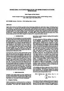
The first data term is the sum of matching cost for all pixels p. The second term adds a constant penalty 𝑃1 for all the neighboring pixels 𝑞 of pixel 𝑝 if the disparity of 𝑞 is different from disparity of 𝑞 by 1. The third data term adds a larger constant value 𝑃2 for all the neighboring pixels q if the disparity difference between 𝑝 and 𝑞 is larger than 1. The problem of stereo matching is formulated as a problem of finding the disparity image D that minimizes the energy function E(D). This global minimization problem is NP-complete and can be efficiently solved using Dynamic Programming (DP) [14]. However, it is well known that this minimization along separate epipolar lines is causing “streaking problem” [14] due to irrelevance of independent processing between image rows. SGM solves this problem by aggregating matching cost from many differentdirections.

D p

H W Figure 1 Cost aggregation. Left: 16 paths cost aggregation at a pixel p in 2D image space. Right: horizontal path cost structure illustration on a single image row.

This is done through summing the costs of all 1D minimum cost paths that end in the pixel 𝑝 at disparity 𝑑 as illustrated in Error! Reference source not found. (left). The matching cost 𝐿𝑟 (𝑝, 𝑑) of pixel 𝑝 at disparity 𝑑 along one particular path is calculated recursively by the following equation: 𝐿𝑟 (𝑝, 𝑑) = 𝐶(𝑝, 𝑑) + min⁡(𝐿𝑟 (𝑝 − 𝑟, 𝑑), 𝐿𝑟 (𝑝 − 𝑟, 𝑑 − 1) + 𝑃1 , 𝐿𝑟 (𝑝 − 𝑟, 𝑑 + 1) + 𝑃1 , min 𝐿𝑟 (𝑝 − 𝑟, 𝑖) + 𝑃2 ) − min⁡𝐿𝑟 (𝑝 − 𝑟, 𝑘) The first term is the matching cost as it is in the energy function E(D). 𝑝 − 𝑟 is the previous pixel along the path. The last term is subtracted from the aggregated cost to avoid number overflow and this term is the same for all the disparities of pixel 𝑝. The final cost of pixel 𝑝 at disparity 𝑑 is the sum of all costs from all paths. S(p, d) = ∑ 𝐿𝑟 (𝑝, 𝑑) 𝑟

2.3. Disparity Computation After computing the matching cost cube, the disparity of a pixel p is determined by selecting the disparity that corresponds the minimum cost from all its disparity search range, that is 𝑚𝑖𝑛𝑑 𝑆[𝑝, 𝑑]. Hence the disparity image that corresponds to the base image 𝐷𝑏 is obtained. The disparity image that corresponds to the match image 𝐷𝑚 can also be determined from the same costs as well by traversing the epipolar line that corresponds to the pixel q of the match image. For sub-pixel disparity accuracy, a quadratic curve is fitted using neighboring costs next to the disparity that has the minimum cost. The occlusions and false matches can be determined by performing a consistency check between 𝐷𝑏 and 𝐷𝑚 . This consistency check enforces the uniqueness constraint by permitting one to one mapping only. Summarizing, the algorithm steps for the SGM computation are: 1. Cost computation 2. Cost aggregation 3. Minimum cost determination 4. Sub-pixel interpolation 5. Median filter 6. Right-to-left consistency check

3. PROPOSED BINARY ADAPTIVE SGM AND EXPERIMENTS The penalty parameters 𝑃1 and 𝑃2 used in original SGM are fixed constants during the aggregation process. We propose to incorporate a binary adaptive property into the original Semi-Global Matching algorithm based on image edges extracted by edge detectors. The edges used in this paper are defined to be points where there is a boundary (or an edge) between two image regions. In another words, we proposed to use smaller penalty parameter at image edges and larger penalty at non-edge areas. This is reasonable since image edges which are typically object boundaries are more likely to indicate depth discontinuity. Thus, smaller penalty should be used at image edges in order to give more freedom and to allow disparity changes. However, it should be also noted that even when edges are detected because of object texture rather than depth discontinuity, the penalty parameters will not affect the disparity estimation since the disparity with the minimum matching cost will remain minimum regardless of what penalty parameters are used there. Hence in our implementation, we have in total three different penalty parameters 𝑃1 , 𝑃2 and 𝑃3 where 𝑃3 > 𝑃2 > 𝑃1 . In the cost aggregation step, 𝑃1 is added to the cost as it does in the original

algorithm for neighboring pixels whose disparity changes a little bit (1 pixel). For the neighboring pixels whose disparity changes more than 1 pixel, 𝑃3 is added to the matching cost if pixel is located at image edges, otherwise the smaller penalty 𝑃2 is added to the matching cost. We carried our experiments on the standard Middlebury stereo datasets, specifically, “cones”, “teddy”, and “tsukuba”. We implemented SGM algorithm in 8 paths rather than 16 paths. Only the median filter is applied after the initial disparity map is obtained from minimum cost selection. The consistency check and sub-pixel interpolation are not implemented because we only want the qualitative justification of the proposed binary adaptive SGM. We use the popular Canny edge detector to extract image edges [15]. The performance of the proposed algorithm improvement is evaluated by comparison of the results with the ground truth to see how much accuracy improvement could be achieved under these conditions. The parameters used in our experiment are 𝑃1 = 5, 𝑃2 = 7, 𝑃3 = 8. We estimated the Root-Mean-Squared (RMS) error using the following equation 1 1 R = ( ∑ |𝑑𝐶 (𝑥, 𝑦) − 𝑑 𝑇 (𝑥, 𝑦)|2 )2 𝑁 (𝑥,𝑦)

Error! Reference source not found. shows the original image, Canny edge image, ground truth, disparity map obtained through original SGM and disparity map through our modified SGM. presents the disparity map evaluation results of the original SGM and our modified SGM. The accuracy of disparity estimation is increased by about 6 to 7 percent as can be seen in the table. Note that this improvement does not require additional computations or memory cost to the original SGM. It is still able to improve the SGM algorithm accuracy performance to a certain degree. It is believed that with both consistency and sub-pixel processing added to the final disparity optimization, the accuracy improvement will become even more significant since the base RMS error becomes smaller. Original SGM

Binary Adaptive SGM

Accuracy Improvement

RMS(cone)

6.494

6.10

6.16%

RMS(teddy)

6.405

6.01

6.25%

RMS(tsukuba)

1.32

1.22

7.58%

Table 1 Disparity map evaluation result

4. POTENTIAL IMPROVEMENTS The Canny detector only indicates presence or absence of sharp gradients in the brightness image with a single parameter – threshold. However, there exist segmentation algorithms which produce a whole hierarchy of edges depending on their strength. In particular the algorithm proposed in [17] segments an image hierarchically thus attributing different strengths to different edges. This allows us to introduce a sequence of penalty parameters instead of single P3. This is a straightforward modification and will be experimented with in near future. Another possible improvement is associated with taking into account individual color channels. According to estimates in [18] this may provide up to 10% more edges compared to grayscale imagery. In general, edge detection in color images is a well-researched subject (see [19] for a review).

5. CONCLUSION In this paper, we propose to use binary penalty parameters based on the image edges extracted by Canny algorithm instead of a single penalty parameter in the Semi-Global Matching algorithm. We experimented with this improvement on the standard Middlebury stereo dataset and evaluated its performance. We have found that this modification increases the accuracy of disparity map estimation by approximately 6 to 7 percent without increase of the computational cost. The implementation of this modification is straightforward and can be integrated into other SGM variants regardless of hardware configurations since

it doesn’t influence the parallelization of the original method. We plan to experiment with more combinations of these three penalty parameters in the future in order to optimize their values for different types of images. More accurate disparity maps could be achieved based on image segmentation results rather than image edges. In addition, incorporating more constraints into the different SGM steps is also considered to be a promising way to improve SGM since currently only smooth constraint and uniqueness constraint are applied in the processing pipeline.

Figure 2 Experiment Results. Top to bottom row: image, Canny edges, ground truth, SGM depth map and depth map

obtained by the reported algorithm. REFERENCES [1] Hirschmuller, H., “Stereo Processing by Semiglobal Matching and Mutual Information”, Pattern Analysis and Machine Learning, 30(2), 328-341(2008). [2] Hirschmuller, H., “Accurate and Efficient Stereo Processing by Semi-Global Matching and Mutual Information”, Proc. CVPR 2, 807-814(2005). [3] Gehrke, S., Morin, K., Downey, M., et al., “Semi-Global Matching: An Alternative to LiDAR for DSM Generation?”, Remote Sensing and Spatial Information Sciences, 38(B1), (2010). [4] Hermann, S., Klette, R., “Iterative Semi-Global Matching for Robust Driver Assistance Systems”, Proc. ACCV, 465478(2013). [5] Ernst, I., Hirschmuller, H., “Mutual Information based Semi-Global Stereo Matching on the GPU”, Proc. Advances in Visual Computing, 228-239(2008). [6] Gibson, J., Marques, O., “Stereo Depth with a Unified Architecture GPU”, Proc. CVPRW’08, 1-6(2008). [7] Spangenberg, R., Langner, T., Adfeldt, S., et al., “Large Scale Semi-Global Matching on the CPU”, Intelligent Vehicles Symposium Proceedings, 195-201(2014). [8] Gehrig, S.K., Rabe, C., “Real-time Semi-Global Matching on the CPU”, CVPRW, 86-92(2010). [9] Michael, M., Salmen, J., et al., “Real-time Stereo Vision: Optimizing Semi-Global Matching”, Intelligent Vehicles Symposium (IV), 1197-1202(2013). [10] Banz, C., Pirsch, P., Blume, H., “Evaluation of Penalty Functions for Semi-Global Matching Cost Aggregation”, Proc. ISPRS 39, B3(2012). [11] Hirschmuller, H., Schastein, D., “Evaluation of Cost Functions for Stereo Matching”, Proc. CVPR, 1-8(2007). [12] Scharstein, D., Szeliski, R., “A Taxonomy and Evaluation of Dense Two-Frame Stereo Correspondence Algorithms”, International journal of computer vision 47(1-3), 7-42(2002). [13] Kim, J., Kolmogorov, V., Zabih, R., “Visual Correspondence Using Energy Minimization and Mutual Information”, Proc. Computer Vision, 1033-1040(2003). [14] Birchfield, S., Tomasi, C., “Depth Discontinuities by Pixel-to-Pixel Stereo”, International Journal of Computer Vision 35(3), 269-293(1999). [15] Canny, J., “A Computational Approach To Edge Detection”, Pattern Analysis and Machine Intelligence (6), 679698(1986). [16] Birchfield, S., Tomasi, C., “A Pixel Dissimilarity Measure That Is Insensitive to Image Sampling”, Pattern Analysis and Machine Intelligence, 20(4), 401-406(1998). [17] Prasad, L., Skourikhine, A.N., “Vectorized image segmentation via trixel agglomeration”, Pattern Recognition, 39(4), 501-514(2006). [18]Novak, C.L., Shafer, S.A., "Color Edge Detection", Proceedings DARPA Image Understanding Workshop Vol. 1, 3537(1987). [19] Mittal, A., Sofat, S., Hancock, E., “Detection of Edges in Color Images: A Review and Evaluative Comparison of Stateof-the-Art Techniques”, Proc of Third Intl Conference AIS 2012, 250-259(2012).