Pacific Symposium on Biocomputing 4:444-455 (1999) ... property that the activity measurement is error prone. The error ... A significant error rate will neutralize.
Pacific Symposium on Biocomputing 4:444-455 (1999)
BINARY QSAR: A NEW METHOD FOR THE DETERMINATION OF QUANTITATIVE STRUCTURE ACTIVITY RELATIONSHIPS P. LABUTE Chemical Computing Group Inc. 1255 University Street, Suite 1600, Montreal, Quebec, Canada H3B 3X3 A new method (particularly suited to the analysis of High Throughput Screening data) is presented for the determination of quantitative structure activity relationships. The method, termed “Binary QSAR,” accepts binary activity measurements (e.g., pass/fail or active/inactive) and molecular descriptor vectors as input. A Bayesian inference technique is used to predict whether or not a new compound will be active or inactive. Experiments were conducted on a data set of 1947 molecules. The results show that the method exhibits high accuracy and is robust to measurement errors.
1
Introduction
The automation of physical experiments through robotics to effectively perform hundreds of thousands or millions of experiments in a short time has opened the door to a large-scale brute-force approach to drug discovery. This approach is generally called High Throughput Screening (HTS). The motivation behind this approach is to reduce, and possibly eliminate, time-consuming and costly manual interventions by physically synthesizing and testing a very large number of compounds. This HTS brute-force ideal can, perhaps, be realized when a few million compounds need to be tested; however, two factors will likely interfere with the HTS ideal: • The number of possible ligands. The number of stable drug candidates is not known. Estimates vary widely; however, the lowest estimate is that there are at least ten trillion reasonable candidates. Even if one million candidates can be tested per day an exhaustive test of all candidates would require ten million days, or more than 27,300 years. A throughput rate of one billion measurements per day would require over 27 years. • The economics of HTS. The cost per HTS measurement is not negligible. The average cost of raw materials and overhead results in a rate of approximately $5 per measurementa. This is certainly a substantial improvement over manual measurement; however, a one-million-test-per-day rate results in a daily expenditure of $5 million (sufficiently high to warrant an attempt at cost reduction).
a
This figure is based upon communications with High Throughput Screening system manufacturers and screening facility operators.
Pacific Symposium on Biocomputing 4:444-455 (1999)
These two factors strongly suggest that “Brute Force HTS” will have to become “Smart HTS” rather quickly. In other words, to reduce the total number of experiments, an experiment/analysis cycle will have to be developed so that, for example, the results of an HTS run on 100,000 compounds are analyzed and used to determine the next 100,000 compounds to be tested. It is generally accepted that the structure, composition, or physical properties of a ligand directly affect its biological activity against a target. The attempt to transform this qualitative belief into a quantitative method of activity assessment is known as the determination of Quantitative Structure Activity Relationships (QSAR) which began with the work of Hanschb and further developed by othersc,d. Determining a QSAR generally proceeds as follows: 1. Define a quantitative measure of activity (e.g., the amount of ligand needed to produce an interference with the functioning of the target). 2. Express the ligand in some quantitative manner; that is, select a collection of numbers that characterize the ligand. These numbers are called molecular descriptors or, descriptors. 3. Determine a functional relationship between activity and the selected descriptors; that is, search for a mathematical function, f, that has the property that “activity = f (descriptors)” to a suitably high level of accuracy. 4. Use the determined activity measure, molecular descriptors and determined functional relationship to predict the activity of new candidate ligands. Currently, QSAR techniques are applied to relatively small data sets consisting of several tens, or perhaps several hundreds, of molecules for which activity measurements are available. These activity measurements are performed manually in the laboratory and produce relatively accurate measurements (e.g., IC 50 numbers: the concentration of ligand required to attain 50% inhibition). The most widely used method of determining the functional relationship is the statistical technique of regressione or least squares. It is natural and tempting to assume that all one needs to do is apply current QSAR methodology to the large scale data sets of HTS and provide the necessary analysis portion of the proposed HTS experiment/analysis cycle. Unfortunately, Hansch,C., Fujita,T. ρ-σ-π Analysis. A Method for the Correlation of Biological Activity and Chemical Structure. J.Am.Chem.Soc. 1964. c Cramer,R.D., Patterson,D.E., Bunce,J.D. Comparative Molecular Field Analysis (CoMFA). 1. Effect of Shape on Binding of Steroids to Carrier Proteins. J.Am.Chem.Soc., 1988, 110, 5959-5967. d Rogers,D.,Hopfinger,A.J., Application of Genetic Function Approximation to Quantitative StructureActivity Relationships and Quantitative Structure-Property Relationships, J.Chem.Info.Comp.Sci., 1994, 34. e Hogg,R.V, Tanis,E.A. Probability and Statistical Inference. MacMillan Publishing Company, New York. 1993. b
Pacific Symposium on Biocomputing 4:444-455 (1999)
two critical factors render the current QSAR technology practically useless for HTS: 1. Precision Loss. HTS has given rise to the following trade-off: higher throughput reduces the precision of the activity measurement. Many HTS technologies report a binary condition: a candidate ligand is either “active” or “inactive.” Some HTS technologies report a discrete measure, e.g., activity on a scale from 1 to 10. In either case, current QSAR technology requires a continuous activity measurement; e.g., accurate to 2 or 3 decimal places. 2. Potentially Significant Error Rate. Many HTS techniques have the unfortunate property that the activity measurement is error prone. The error rate is significant enough to warrant special attention since current QSAR technology is very sensitive to outliers and errors. A significant error rate will neutralize the predictive capabilities of current QSAR technology. Consider a simple example. Suppose that activity y is linearly related to a single descriptor x; that is, y = mx + b. A conventional data set would consist of n observations (yi,xi). Without loss of generality we may assume that m > 0, the xi have mean 0 and variance 1 and that activity is indicated by the condition that y < 0 (i.e., when x < -b/m). The linear regression estimates for m and b are 1 n 1 n mˆ = ∑ yi xi , bˆ = y , y = ∑ y i (1) n i =1 n i =1 When presented with binary measurements (1 is active, 0 is inactive) representing the condition that yi < 0 the linear regression estimates become a 1 mˆ = (2) ∑ xi , bˆ = n xi 0 is
∏
m
Bk =
∑
δ ( z i ∈ (bk −1 , bk ]) =
i =1
m
bk
∑ ∫ δ ( x − z )dx i
(8)
i =1 bk −1
which has unfortunate sensitivity to the selection of bin boundaries since observations close to the boundary between two bins are treated as if they were in the middle of one of the bins. To reduce the sensitivity to the bin boundaries we 2 replace the delta function observation density with a Gaussian with variance σ (this can be interpreted as an observation error as well as a smoothing parameter). We now have m
Bk =
bk
∑∫σ i =1 bk −1
1 ( x − zi ) 2 exp − dx 2 2π 2 σ
1
bk − z i erf σ 2 i =1 which is more efficiently calculated with 1 = 2
m
∑
b − zi − erf k −1 σ 2
(9)
bk − z i . (10) 2 i =1 Even with this smoothing, it may happen that some bins are essentially 0. We therefore construct the final distributions by adding a constant to each bin before normalizing (similar to the Bayes estimate of a). Thus, the discrete density for Z is estimated with Bk = E k − E k −1 ,
Ek =
Pr( z ∈ (bk −1 , bk ]) ≈
1 2
m
∑ erf σ
Bk + 1 / c , c= c+ B/c
B
∑B
l
l =1
Finally, to evaluate the density f at a particular point, z, we calculate
(11)
Pacific Symposium on Biocomputing 4:444-455 (1999)
f ( z ) ≈ fˆ ( z ) =
2 Bk + 1 / c bk 1 ( x − z ) exp− dx ∫ 2σ 2 k =1 c + B / c bk −1 σ 2π B
∑
(12)
which simplifies to
b − z bk − z − erf k −1 (13) 2 σ 2 k =1 We can thus model each of the descriptor distributions fj(x,y) for y in {0,1} and j in {1,…,n}; that is, for each descriptor, we estimate two distributions: one for the active molecules in the training set and one for the inactive molecules. We thus arrive at the estimate 1 fˆ ( z ) = 2
B
Bk + 1 / c
∑ c + B / c erf σ
−1
m + 1 n fˆ j ( x j ,0) . p( x) ≈ 1 + 0 m1 + 1 j =1 fˆ j ( x j ,1) The above considerations suggest the following computational procedure:
∏
(14)
1.
For each molecule in the experimental data set, compute di = D(Li).
2.
Perform a principal component analysisg to produce a matrix Q and a vector u such that the covariance matrix of {xi = Q(di-u)} is the identity matrix.
3.
Estimate the parameters of the probability model, p, from {(yi,xi)}.
4.
The probability that a new molecule L is active is then estimated as p(Q(D(L)-u)).
3
Results and Discussion
A set of 1,947 small molecules with molar refractivity data were chosen to test the correctness and robustness to measurement error of the method. The range of molecular weights in the data set was (28,1609) with a mean weight of 312 and a standard deviation of 131. The molar refractivity values were in the range (0.3,30) with a mean of 8.3 and a standard deviation of 3.27. An inactivity criterion of yi > y0 was used to create a binary experimental value; that is, if the molar refractivity was greater than a pre-set threshold then the molecule was considered inactive. Several values of y0 were chosen which resulted in different divisions of the data set into active and inactive (between 51% and 97.5%). Table 1 gives the threshold values used in the experiments and the percentage of molecules in the data set that were, as a result, classified as inactive.
g
Glen,W.D, Dunn,W.J., Scott,R.D. Principal Components Analysis and Partial Least Squares Regression. Tetrahedron Comput. Methodol., 1989, 2, 349-376.
Pacific Symposium on Biocomputing 4:444-455 (1999)
y0 2.650 2.975 3.300 3.625 3.950 4.275 4.600 4.925 5.250
% > y0 97.48 97.02 96.46 95.07 93.07 90.24 87.78 85.82 83.05
y0 5.575 5.900 6.225 6.550 6.875 7.200 7.525 7.850 8.175
% > y0 80.28 77.04 73.70 70.31 67.13 63.79 60.25 56.09 51.52
Table 1. Proportion of inactive compounds as a function of the threshold.
Four molecular descriptors were chosen to represent the molecules: two zero’th order and two first order connectivity indicesh defined as follows:
χ 0 = ∑ d i−1 / 2
χ1 = ∑ (d i d j ) −1 / 2
χ 0v = ∑ si−1 / 2
χ1v = ∑ ( si s j ) −1 / 2
i
i
ij
(15)
ij
where d is the number of heavy atoms connected to atom i and s = (v-h) / (Z-v-1), where Z is the atomic number, h is the number of attached hydrogens, and v is the number of valence electrons. The sums over ij denote summation over all heavy atom bonds i-j. The descriptors were calculated using the 1998.03 version of the MOEi software from Chemical Computing Group Inc (the descriptor codes used were chi0, chi1, chi0v, chi1v). The prediction method was implemented using the SVL programming language built into MOE. For each threshold value y0 a predictive model was estimated (with Gaussian smoothing parameter σ = 0.25 ) and evaluated against the data set. Estimation of model parameters required approximately 2 seconds of CPU time for each threshold value. Performance was measured as follows. Let m0 be the number of inactives in the data set and m1 the number of actives. Let c0 be the number of inactives correctly labeled by the model and let c1 be the number of actives correctly labeled by the model. Performance is measured with the following three percentages: a = 100(c0+c1)/(m0+m1) the percentage of correctly predicted activity values over all of the data, a0=100c0/m0 the percentage of correctly predicted activity values over the inactive molecules only, and a1=100c1/m1 the percentage of correctly predicted activity values over the active molecules only. Figure 1 summarizes these results. h i
Bicerano,J., Prediction of Polymer Properties, Marcel Decker Publishing, New York, 1996. Consult http://www.chemcomp.com for more information.
Pacific Symposium on Biocomputing 4:444-455 (1999)
100 98 96 % Correct
94 92 90 88 86 84 82
All Data
Actives Only
Inactives Only
74 80 86 90 % Inactive in Data Set
95
80 52
60
67
97
Figure 1. Proportion of inactive compounds as a function of the threshold.
At all threshold values yi, accuracy is extremely significant (statistically) and well above what is expected from random assignments using the percentage of actives in the data set. Overall accuracy was between 91% and 99.5%. More importantly, the accuracy on the active subset was between 93% and 99.5%. Accuracy in the inactive subset was between 83.5% and 99.5%. It should be noted that the drop in accuracy in the active subset (in the right-most portion of the graph) was probably due to the fact that very few molecules were used to estimate the active distributions. This small sample fall-off would likely be eliminated with a larger data set. When the number of actives in the data set was below 10% the model performed very well with all accuracy measures above 90% correct. To measure the sensitivity of the method to errors in the measured activity values, the following procedure was used. To each refractivity value yi a uniform random error was introduced in the range [-ws,ws] where s is the standard deviation of the refractivity values and w is a pre-set error scale factor. This resulted in an activity criterion of yi + ei > y0 where ei is uniform in [-ws,ws]. The data set was trained on the modified data and accuracy measured against the actual criterion yi > y0. Three values of w were used: 0.1, 0.5 and 1.0. Each value of w was used 10 times for each value of y0 and the accuracy results averaged. Figure 2 presents the accuracy results for the entire data set.
% Correct
Pacific Symposium on Biocomputing 4:444-455 (1999)
100 98 96 94 92 90 88 86 84 82 80
w=0.0
52
60
67
w=0.1
w=0.5
74 80 86 90 % Inactive in Data Set
w=1.0
95
97
Figure 2. Accuracy results for entire data set with uniform errors.
% Correct
At all error widths of w overall accuracy is maintained between 90% and 99.5%. Figure 3 presents the accuracy results on the active subset of the data for each of the w values. 99 97 95 93 91 89 87 85 83 81 79 77 75
w=0.0
52
60
67
w=0.1
w=0.5
74 80 86 90 % Inactive in Data Set
w=1.0
95
97
Figure 3. Accuracy results for actives only with uniform errors.
High statistical significance was maintained at all error rates and reasonable accuracy was maintained. The active-only subset showed some accuracy fall-off at very large error widths in the small sample region of the plot (lower right). This was probably due to the small number of actives that were used to estimate the
Pacific Symposium on Biocomputing 4:444-455 (1999)
probability distributions. Despite this fall-off, it is clear that the method is capable of withstanding very high levels of measurement error in the data set. Another form of error generation was tested. Each activity measurement was randomly inverted with probability p; that is, active and inactive was reversed for randomly selected data points. Error rate values of 5% and 10% were used. Each error rate was used 10 times and the accuracy results averaged. Figure 4 presents the overall accuracy rates for each of the error rates. 100 98 96 % Correct
94 92 90 88 86 84 82 p=0%
p=5%
p=10%
80 52
60
67
74 80 86 90 % Inactive in Data Set
95
97
Figure 4. Accuracy results for entire data set with inversion errors.
At both error rates the accuracy on the entire data set was maintained and fell between 92% and 99.5%. It is interesting to note that the overall accuracy was better when some errors are introduced in the cases where the number of actives was below 10%. This suggests that it might be possible to improve the overall accuracy by data smoothing techniques (e.g., addition of “constructive noise”) that directly model sources of error; i.e., one can take into account knowledge that there is a 5% error rate. Figure 5 presents the accuracy results of the same experiments on the active subset.
Pacific Symposium on Biocomputing 4:444-455 (1999)
100 98 96 % Correct
94 92 90 88 86 84 82
p=0%
p=5%
p=10%
80 52
60
67
74 80 86 90 % Inactive in Data Set
95
97
Figure 5. Accuracy results for actives only with inversion errors.
High significance is maintained at both error rates with accuracy on the active subset falling between 81% and 98%. As with the previous results, the observed accuracy fall-off was likely due to small sample effects. It must be emphasized that this fall-off is rather minor and very high statistical significance is maintained even with the small sample size. All calculations were performed with MOE 1998.03 on a Compaq Pentium 133 with 32Mb of memory running Windows95. 4
CONCLUSIONS
A new method for QSAR analysis called Binary QSAR was presented along with results that strongly suggest the method’s accuracy and robustness to measurement error. Future work will attempt to characterize the effect of the smoothing parameter upon accuracy. In the present formulation the smoothing parameter is a free parameter. As such, it can be optimized for a particular data set with a crossvalidation procedure. It may be possible to eliminate the smoothing parameter by making it a function of, perhaps, the bin widths or the number of data set points. A notable drawback of Binary QSAR is that there is no obvious way to determine the relative importance of the descriptors. In linear regression analysis, for example, each descriptor is assigned a single coefficient that can be used to estimate descriptor relevance. On the other hand, since Binary QSAR is a nonlinear modeling method there is no analogous coefficient. Assessing the relative importance of the descriptors will be the subject of future work. Binary QSAR is a fundamental shift away from the empirically fitted functional relationship methods of traditional QSAR methodology. Rather than fitting the
Pacific Symposium on Biocomputing 4:444-455 (1999)
parameters of a model to experimental data, Binary QSAR builds predictive binary models through the use of large-scale probabilistic and statistical inference. Because data fitting is not used, the predictive capacity of Binary QSAR is not interpolative, but based on generalizations substantiated by the experimental data. Binary QSAR has several important and immediate applications: • Prioritization of HTS Experiments. Rather than test, for example, 5,000,000 compounds in a single run, break up the set of 5,000,000 compounds into lots of, say, 50,000 compounds. Binary QSAR could then be used to estimate the number of active compounds, or hits, in lots that have not been tested. In this way hits are found earlier and subsequent HTS experiments are more focused. Each HTS experiment proceeds from maximal diversity in the tested compounds to minimal diversity focusing on the discovered hits. • Combinatorial Library Design. It is often the case that combinatorial chemistry techniques are used to create candidates for HTS experiments. Current combinatorial library design methods focus on maximizing the diversity of the resulting collection of compounds. Using Binary QSAR facilitates the design of more focused combinatorial libraries: the data from an HTS experiment is used to bias the combinatorial library towards diverse, but active, compounds. • Virtual Screening and Virtual Synthesis. Once a Binary QSAR analysis is performed on HTS results, the resulting data model is used to search for other active compounds in corporate or supplier databases or even reaction pathways. Chemical Computing Group has sought patent protection for the Binary QSAR methodology. Binary QSAR is available in Chemical Computing Group’s MOE software as QuaSAR-Binary™ and may be licensed from Chemical Computing Group Inc.