MARINE ECOLOGY PROGRESS SERIES Mar Ecol Prog Ser
Vol. 331: 291–304, 2007
Published February 16
REVIEW
Biodiversity of benthic assemblages on the Arctic continental shelf: historical data from Canada Mathieu Cusson1, 4, Philippe Archambault2, 5,*, Alec Aitken3 1
Département de Biologie, Québec-Océan (GIROQ), Université Laval, Québec G1K 7P4, Canada Sciences de l’Habitat, Institut Maurice-Lamontagne, Pêches et Océans Canada, CP 1000, Mont-Joli, Québec G5H 3Z4, Canada 3 Department of Geography, University of Saskatchewan, 9 Campus Drive, Saskatoon, Saskatchewan S7N 5A5, Canada 4 Present address: School of Biology and Environmental Science, University College Dublin, Belfield, Dublin 4, Ireland 5 Present address: Institut des Sciences de la Mer de Rimouski (ISMER), Université du Quebec à Rimouski, 310 Allée des Ursulines, Rimouski, Quebec G5L 3A1, Canada
2
ABSTRACT: This study describes patterns of abundance, diversity, and assemblages of benthic macrofauna within the Canadian Arctic Archipelago. A review of data reports and the published literature yielded 219 stations and 947 taxa from 7 sources in various regions of the Canadian Arctic Archipelago (i.e. Beaufort Sea and Mackenzie Shelf, Victoria Island, Hudson and James Bays, Frobisher Bay, Ungava Bay, and Southern Davis Strait). In general, we observed that eastern regions of the Canadian Arctic Archipelago showed greater values of species richness (or α diversity) than the western and central regions, whereas no specific patterns were observed for Shannon-Wiener’s diversity (H’) and Pielou’s evenness (J’) indices. The Beaufort Sea and Mackenzie Shelf region exhibited high values of taxonomic distinctness (Δ+), whereas Hudson Bay showed low values. However, the Hudson Bay region showed high values of turnover (βW) diversity. A non-metric multi-dimensional scaling plot of similarity (Bray-Curtis index) and analysis of similarity revealed that species composition differed among regions, even those located in close proximity to one another. These investigations were conducted at different levels of taxonomic resolution (Species, Order, Class and Phyla) and the results demonstrated that most patterns were maintained up to the Order and Class level. A relatively small number of taxa, mainly annelids, were responsible for most of the dissimilarity among regions. Bottom salinity and temperature were the most important environmental variables (among depth of site, bottom temperature, salinity, physical and chemical sediment characteristics) for determining these assemblage patterns. Multiple regression analyses also demonstrated that variance in species richness and diversity (H’) was best explained by variance in salinity (55 and 43% respectively). The analysis of a time series from Frobisher Bay revealed that the temporal (mo/yrscale) variability of assemblages was of the same order as the spatial (km-scale) variability among sites. KEY WORDS: Benthic assemblage · Meta-analysis · Historical data · Arctic macrobenthos · Multivariate analysis · α, γ, and turnover (β) diversity · Spatial and temporal variability Resale or republication not permitted without written consent of the publisher
Within the last 2 decades, research on the macrobenthos of the Arctic continental shelves has shifted from being largely descriptive to a process-oriented approach (e.g. Piepenburg 2005). Baseline information such as species inventories, patterns of abundance, and
comparisons of biodiversity among Arctic regions remains difficult to find. Furthermore, despite the urgency to address observations of biodiversity patterns at larger scales (i.e. global Canadian Arctic), the emphasis of biodiversity research on the Arctic benthos has been focused at local to regional scales (e.g. Bluhm et al. 2005, Conlan & Kvitek 2005). Research at a
*Corresponding author. Email:
[email protected]
© Inter-Research 2007 · www.int-res.com
INTRODUCTION
292
Mar Ecol Prog Ser 331: 291–304, 2007
broader scale has been impeded by 2 major factors. The first is the considerable technical difficulty of sampling the Arctic environment at scales greater than local or regional; the only way to solve this problem is to gather and compare data from many studies and/or use historical data. The second is that the richly diverse fauna requires great taxonomic skills to provide a consistent and reliable inventory. If these 2 factors could be overcome, the description of past variability in benthic community structure may help to track future potential modifications brought about by changes (i.e. increasing temperature and sea level, glaciers melting, etc.) experienced at large scales in the Arctic environment (e.g. Moritz et al. 2002, ACIA 2005, Polyakov et al. 2005). Many proxies have been used to follow changes in the environment, including the Shannon-Wiener diversity index (H’) and species richness. These are widely used and considered to be good indicators of community structure. Recently, biodiversity has been related to spatial scale using various measurements (e.g. α, γ and turnover [β] diversity) (e.g. Gray 2000, Magurran 2004). However, these univariate variables may stay constant whereas species composition may change (e.g. Clarke & Warwick 2001a, Bertocci et al. 2005). Indeed, multivariate analyses can often reveal or illustrate patterns in diversity and species richness where univariate analyses cannot (Gray et al. 1990). It has become common to use measures of community assemblage similarities (in term of species composition and abundance) to circumvent the loss of information inherent in univariate summaries of community structure (Downes et al. 2002). Changes in species composition and dominance in benthic communities have been detected along environmental gradients (e.g. Warwick & Clarke 1993), or in response to pollution disturbance (e.g. Warwick & Clarke 1993, Harkantra & Rodrigues 2004) and natural spatial variability (e.g. Somerfield & Gage 2000, Clarke & Warwick 2001a). Multivariate analyses are more robust at detecting transformations that can occur in species abundance and dominance in a community. Applying such tools to historical data may provide insights into the state of historical communities. Historical data from the Canadian Arctic Archipelago include long-term field experiments on the effects of oil spillage in arctic waters (e.g. Cross et al. 1987, Cross & Thomson 1987), as well as quantitative (density and biomass) studies of benthos across the continental shelf and slope (Thomson 1982, Dunton et al. 2005) and within fjords (Syvitski et al. 1989, Aitken & Fournier 1993). There has been a progressive thinning and shorter duration of sea ice cover in the Arctic in general (e.g. Serreze et al. 2003, Comiso & Parkinson 2004) and in many of the Canadian Arctic regions (e.g. Barber & Hanesiak 2004, Belchansky et al. 2004, Gagnon & Gough 2005). This, coupled with the likely
future exploitation of the Canadian Arctic for marine transport, has created a need to establish baseline data on the state of the marine environment using new statistical tools for comparisons with contemporary studies. To achieve this goal, the importance of using grey literature (e.g. technical reports, government documents, unpublished manuscripts) to enlarge the database should not be underestimated. The objectives of this paper were to use such data to: (1) characterize and evaluate differences in benthic macrofaunal species richness, α, β and γ diversity, and assemblages from historic data sets within the Canadian Arctic regions; (2) compare the relative importance of spatial and temporal variability of species assemblages from those sites with temporal data; and (3) evaluate the correlation between benthic assemblages and the environmental variables for which we have good information.
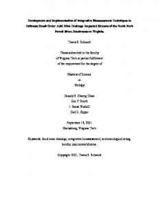
MATERIALS AND METHODS Faunal samples. The literature on historical data related to Canadian Arctic benthos was reviewed. We retained sites for which macrobenthos community data sets from marine and estuarine environments in the Canadian Arctic were available (Table 1). Only data from standardized grabs (van Veen, Ponar, Eckman etc.) were retained to enable comparisons among sites. A total of 219 stations were used (Table 1, Fig. 1). Each station was represented by 1 to 10 grabs (median: 4.5) for which the sampled areas were between 0.09 and 1.2 m2 (median: 0.25). Mean densities per station were used. Most data sets used in this study are from technical reports of the Department of Environment and Fisheries and Oceans Canada, but data from some regions (Southern Davis Strait and Ungava Bay) are from published literature (Stewart 1983, Stewart et al. 1985). Data were obtained from many regions (Beaufort Sea and Mackenzie Shelf: BM; Victoria Island: V; Hudson Bay: HB; James Bay: JB; Ungava Bay: UB; Frobisher Bay: F; Southern Davis Strait: DS) and allowed a broad east –west comparison of benthic assemblages across the Canadian Arctic. Information from some of the regions (e.g. Victoria Island, Hudson Bay) consists only of presence/absence information for each species (i.e. simple species lists). Four sampling time series (with 2, 5, 9, and 10 dates) from Frobisher Bay were available. Delimitation of these regions was mainly based on the zoogeographic subdivision of Canadian Arctic mollusc fauna from Lubinsky (1980) (with a subdivision for Frobisher and Ungava Bay) as well as the Arctic and the sub-Arctic regions described by Curtis (1975). When available, physical data associated with biological data (e.g. depth, bottom temperature and
293
Cusson et al.: Arctic benthic assemblages
Table 1. Stations from the Canadian Arctic included in meta-analysis. L: list of species; D: mean density per species Regions
Date (no. of stations)
Total no. stations per region
Type of data set
61
La
1: Atkinson & Wacasey (1989a)
17 10 101
Db,c,f D & La Db – e
2: Wacasey et al. (1976) 3: Atkinson & Wacasey (1989b) 4: Wacasey et al. (1977)
Hudson Bay (HB)
1955 (1); 1958 (4); 1959 (1); 1961 (6); 1965 (49) James Bay (JB) 1974 (17) Victoria Island (V) 1967 (4); 1968 (4); 1969 (2) Beaufort Sea and 1971 (6); 1973 (17); 1974 (16); Mackenzie Shelf (BM) 1975 (62) Frobisher Bay, 1967 (1); 1968 (8); 1969 (7); Baffin Island (F) 1970 (2) Frobisher Bay, 1969 (2); 1970 (2); 1972 (2); Baffin Island (F) 1973 (7); 1976 (2) Southern Davis Strait (DS) 1977 (13) and Ungava Bay (UB)
Source
5A Db
5: Wacasey et al. (1979)
Db Df
6: Wacasey et al. (1980) 7: MacLaren MAREX (1978)
6B 13
Grab type used: aunspecified grab; bPetterson; cWildco Peterson; dWildco Ponar; eEkman; fvan Veen A includes 2 stations with 5 and 9 sampling dates, respectively; Bincludes 2 stations with 2 and 10 sampling dates, respectively Source*
1 2 3 4 5 6 7 7
Iqualuit
Region names
1 km
Hudson Bay James Bay Victoria Island Beaufort Sea/Mackenzie Frobisher Bay (F6-F12) Frobisher Bay (F1-F5) Southern Davis Strait Ungava Bay
° 85
F1 F2 F3
ee Gr
Monument Island
Long Island F4 F5
nla
Arctic Ocean
Mair
nd
Beaufort Sea and Mackenzie Shelf
F8
F9 Island F6 F7 F10
63°40'N
° 75 68°30'W
Baffin Bay
Cairn Island F11
°
70 0°
14
13
Victoria I.
Ba ffin I.
0° 12 0
Coronation Gulf
°
° 65
x8
Davis Strait
Frobisher Bay
138°
° 60
132°
71° 7
Ungava Bay ° 55
Hudson Bay
°
60
70°
x15
69°
90°
1000 km
James Bay
Inuvik
50°
100 km
80°
Fig. 1. Sampling sites in the Canadian Arctic; *see Table 1 for sources
294
Mar Ecol Prog Ser 331: 291–304, 2007
salinity, and for some stations the chemical properties of the sediment) were examined. For 12% of the stations, bottom temperatures were obtained from the nearest station during the same time period. Based on the method used by the different research groups, all samples were sieved through a 500 µm mesh sieve, and macrofauna sorted under a stereomicroscope (method described in detail in the particular references used). Taxonomic names were checked and updated (e.g. for old or sister names) using data retrieved from the Integrated Taxonomic Information System on-line database (www.itis.gov) and other general invertebrate references (e.g. Barnes 1987, Pechenik 1991). Most data came from the same research groups (Arctic Biological Station, Department of Fisheries and Oceans Canada: sources 1 to 6, see Table 1), which ensured consistency in the taxonomic resolution and identification of organisms. Following Gray’s (2000) terminology, the α diversity (SRS) measurement represents species richness (S: number of species) from samples from a defined area and was associated with each site from a given ‘larger area’ or region; γ diversity (SRL), which includes a variety of habitats and assemblages, is represented by the total number of species from each region. Total species richness (SRT) represents the total number of species included in this study. The turnover (β) diversity, which describes how species similarity changes along an environmental gradient or between habitats, was assessed using Whittaker’s βW diversity (βW = SRL/SRS). Bray-Curtis-similarity (%) between all pair-wise combinations of sites from a given region was also used as a measure of turnover diversity (Mumby 2001, Thrush et al. 2001, Ellingsen & Gray 2002) and is considered to be a good measure (Magurran 2004). Data analysis. One-way analysis of covariance (ANCOVA; GLM and MIXED procedure, SAS 1999) was used to compare total density (ind. m–2), species richness or α diversity (SRS: number of species), Shannon-Wiener’s diversity index (H’, loge), and Pielou’s evenness index (J’: H’/logSRS) among regions using water depth and bottom temperature as covariates. Average taxonomic distinctness (Δ+) and variation in taxonomic distinctness (Λ+), which estimate the average distance between 2 randomly chosen organisms through Linnean taxonomy, were determined with presence/absence data (DIVERSE analyses, PRIMER v5, Clarke & Gorley 2001). These 2 measures are more relevant than the univariate measures mentioned below when assessing biodiversity from an unequal sampling effort, and provide valuable tools to compare historical data and/or meta-analyses over large spatial and temporal scales (Clarke & Warwick 1998, 2001a, b). Tukey-Kramer multiple comparisons tests (SAS 1999) were carried out to determine mean differences among regions. Multiple regression analyses were
used to link abiotic parameters to biotic variables. Step-wise multiple regressions (REG procedure, SAS 1999) were used to examine the relationships between dependent variables (total density, SRS, H’ and J’) and environmental conditions (temperature, salinity, water depth of sampling site, percentage of sand, silt and clay, and chemical characteristics of the sediment). Robustness of the regression models was evaluated by the leave-one-out cross-validation method (Stone 1974). This test systematically excludes 1 data point at a time and predicts its value using the regression model adjusted to the remaining data set. Normality was verified using Shapiro-Wilk’s test (Zar 1999), and homoscedasticity was confirmed by graphical examination of residuals (Scherrer 1984, Montgomery 1991). Methods of Clarke & Warwick (1994, 2001a) using the PRIMER software (Clarke & Gorley 2001) were used to detect spatial and temporal patterns in community structure. Before similarity comparisons among stations were conducted, we discarded species or taxonomic groups (n = 315) associated with only 1 station as suggested by the authors. Faunal data were 4th-root transformed prior to analyses to avoid the strong impact of common species, as recommended by Field et al. (1982). Differences in the structure of benthic assemblages among various regions within the Canadian Arctic were identified by non-metric multidimensional scaling (nMDS) ordination using the Bray-Curtis similarity measure (Bray & Curtis 1957, Clarke 1993). Analyses of similarity (ANOSIM) tested the significance of differences among regions or groups of samples from a given region. For regions where environmental variables were available (i.e. Beaufort Sea and MacKenzie Shelf, James Bay and Frobisher Bay), Spearman’s rank correlations were used to examine relationships with ordination scores (BIO-ENV analyses, PRIMER). For this analysis, biotic and abiotic matrices were constructed using Bray-Curtis dissimilarity (4th-root transformed) and Euclidean distances respectively (see Clarke & Ainsworth 1993, Clarke & Warwick 2001a). Spearman’s rank correlations were also used to examine the relationship between ordination scores and the taxa that best explained the observed pattern of community similarity. The contribution of each species (or higher taxonomic level) to the average Bray-Curtis dissimilarity between regions (or groups of sites) was assessed (SIMPER analyses, PRIMER). A significance threshold of α = 0.05 was adopted for all statistical tests.
RESULTS A total (SRT) of 947 species or taxonomic groups (within 229 different families, 68 orders, 29 classes and 15 phyla) were present at the stations examined in this
295
Cusson et al.: Arctic benthic assemblages
study (n = 219). Arthropoda and Annelida represented 45 and 31%, respectively, of all species included in our database. Benthic composition varied from west to east across the study region, with an average composition of 37% Annelida and 31% Arthropoda (Fig. 2). With the exception of DS, we observed a greater proportion of Arthropoda in the eastern regions (UB and F) than in the central regions (V, HB and JB), where Annelida dominated.
β) diversities, Density, α (SRS), γ (SRL) and turnover (β H’ and J’ indices and taxonomic distinctness The use of covariates did not relate to densities, and only bottom temperature was retained in the ANCOVA for J’ (see Table 2). All univariate variables revealed differences among regions (Table 2, Fig. 3). The largest densities of organisms were observed in F, probably due to the large number of Nemata (Nematoda) (up to 9.4 × 10³ ind. m–2), whereas the lowest densities were observed in JB (Fig. 3a). High species richness (or α diversity: SRS) was observed in the eastern regions (UB, F and DS) and in the V region, whereas low values of SRS were observed in HB (Fig. 3b). The BM region exhibited low diversity (H’), whereas high diversity was observed in the V and F regions. All other regions exhibited intermediate values (Fig. 3c).
Table 2. Summary of ANOVA/ANCOVA with bottom temperature and water depth as covariates, showing effects of: (a) density; (b) species richness (SRS); (c) diversity (H’); (d) evenness (J’); (e) average taxonomic distinctness (Δ+); and (f) variation in taxonomic distinctness (Λ+). Density and species richness were log transformed; depth was square-root transformed to normalize and homogenize the data Source of variation
df
MS
F
(a) Density Regions 5 6.59 15.44 Error 165 0.43 (b) Species richness (SRS) Bottom temperature 1 2.78 20.61 Water depth 1 0.82 6.07 Regions 6 8.68 64.19 Error 227 0.14 (c) Diversity (H’) Bottom temperature 1 7.80 17.18 Water depth 1 3.90 8.59 Regions 5 2.66 5.86 Error 165 0.45 (d) Evenness (J’) Bottom temperature 1 0.12 5.40 Regions 5 0.11 5.23 Error 160 0.02 (e) Average Δ+ Regions 6 1652 3.55 Error 229 465 Λ+) (f) Variation in taxonomic distinctness (Λ Regions 6 308873 7.07 Error 229 43686
p
< 0.0001
< 0.0001 0.0145 < 0.0001
< 0.0001 0.0039 < 0.0001
0.0214 0.0002
0.0022
< 0.0001
100 90
Composition (%)
80 70 60 50 40 30 20 10 0 BM
V
HB
JB
UB
F
DS
All
Geographical regions Arthropoda
Annelida
Mollusca
Echinodermata
Others
Fig. 2. Composition of macrozoobenthic phyla from various regions in the Canadian Arctic. From west to east, BM: Beaufort Sea and Mackenzie Shelf; V: Victoria Island; HB: Hudson Bay; JB: James Bay; UB: Ungava Bay; F: Frobisher Bay; DS: Southern Davis Strait; ‘Others’ included Brachiopoda, Chordata, Cnidaria, Echiura, Ectoprocta, Nemata (Nematoda), Nemertea, Platyhelminthes, Porifera, Priapula, and Sipuncula
High evenness (J’) was observed in the JB and DS regions, whereas lower values were seen in the F and UB regions (Fig. 3d). Although the BM region exhibited low diversity (Fig. 3c) and moderate SRS (Fig. 3b), a high average taxonomic distinctness (Δ+) was observed in this region (Fig. 3e). Low values of Δ+ were observed in the HB region. Low values of variation in taxonomic distinctness (Λ+) were found in the BM and HB regions, whereas high values were observed in the eastern regions (UB, F, and DS; Fig. 3f). The highest γ diversity (SRL) was observed in F, whereas the lowest was found in JB (Table 3). High turnover (β) diversity values were observed in HB (i.e. high βW and low pair-wise BrayCurtis similarities), whereas low values were found in the V and eastern regions (F, UB and DS; Table 3). Multiple linear regression models explained up to 31% of total macroinvertebrate density variance, up to 58% of species richness (SRS) variance, 43% of diversity (H’) variance, and 20% of evenness (J’) variance (Table 4). Variance in total macroinvertebrate density was best explained by bottom temperature variance (12%). Species richness and diversity variance were best explained by variance in salinity (55 and 43% respectively). The evenness variance was equally
296
Mar Ecol Prog Ser 331: 291–304, 2007
5.0
2.5
b
4.5
a,b,c
a,b
3.5 b,c
3.0
b,c c
a,b
1.5
2.0
a,b
b
b
1.0 c
0.5
2.5
0.0 BM V
JB UB
F
DS
BM V HB JB UB F DS
3.5
0.9
c a
3.0
a,b
a,b
a,b,c a,b
Benthic assemblages
b,c
0.7
J'
H'
a
a
a,b b
2.0
d
a,b,c
c
0.6
1.5
0.5
1.0
0.4 BM V
ea
explained by variance in the percentage of silt and in the nitrate and ammonia content of the sediment. When only the chemical characteristics of the sediment were included in models (see second models in Table 4, where salinity, temperature, water depth and percentage of silt were not included [NI]), potassium and ammonia content were important variables, accounting for the remaining variance in total density, species richness and diversity values.
0.8
2.5
90
a,b a
2.0 a
4.0
SRS (log10)
Density (log10)
a
JB UB
F
DS
BM V 700
a,b
a,b
a,b
85
a,b
JB UB
f
DS a,b
600
a
a,b
a,b
80
F
a,b,c
500 a,b,c
b
75
400
70
300
b,c c
65
200 BM V HB JB UB F DS
BM V HB JB UB F DS
Geographical regions Fig. 3. Least-squared mean of: (a) density (ind. m–2); (b) species richness (SRS); (c) Shannon-Wiener’s diversity index (H’); (d) Pielou’s evenness index (J’); (e) average taxonomic distinctness (Δ+) (presence/absence data); and (f) variation in taxonomic distinctness (Λ+) (presence/absence data) for each geographical region, see Fig. 2 for region abbreviations. Dashed line in (e) and (f) indicates values of Δ+ and Λ+ from the master list of 947 taxa. Note: for HB, only SRS, Δ+ and Λ+ were estimated due to the nature of the data (species list). Error bars: ± SE; different letters (a,b,c) above points indicate significant differences (p < 0.05)
Results revealed that HB, JB and BM had very peculiar species compositions with a wide spectrum of assemblages (Fig. 4). The species composition of the JB region was more similar to that of the BM communities than to that of HB, which is closer spatially. However, ANOSIM analyses (Table 5) revealed that the assemblages of the HB and JB regions were dissimilar only at the species level but not at the order or other higher taxonomic levels, whereas the assemblages of HB and BM were dissimilar at all levels of taxonomic resolution (Table 5). We did not observe any differences in presence/ absence data between JB and BM at any level of taxonomic resolution. No major differences were observed in the nMDS plots (excluding HB sites, for which only species lists were available) (compare Fig. 4b with Fig. 4a). F stations (s) were restricted to a small area in all nMDS plots (Fig. 4), and ANOSIM indicated that the F region had a distinct benthic community composition relative to all other
Table 3. γ diversity (SRL) and measures of turnover (β) diversity for each region using mean Whittaker’s (βW) diversity and mean Bray-Curtis similarity (%) between all pair-wise comparisons of sites. CI: 95% confidence intervals γ diversity SRL Region Beaufort Sea and Mackenzie Shelf (BM) Victoria Island (V) Hudson Bay (HB) James Bay (JB) Frobisher Bay (F) Ungava Bay (UB) Southern Davis Strait (DS) Total of taxa from all regions (=SRT)
327 167 167 104 434 232 312 947
Turnover (β) diversity βW (SRL /SRS) Bray-Curtis similarity (%) Mean ± CI Mean ± CI 42.2 ± 11.1 3.9 ± 1.2 62.4 ± 13.8 18.2 ± 11.6 5.7 ± 1.4 2.1 ± 0.8 5.9 ± 2.4
17.8 ± 0.5 38.9 ± 4.3 6.2 ± 0.6 18.4 ± 2.3 47.8 ± 3.9 36.6 ± 5.0 29.4 ± 3.3
H’ = Partial R2 H’ = Partial R2 J’ = Partial R2
Log (TD) = Partial R2 Log (TD) = Partial R2 Log (SRS) = Partial R2 Log (SRS) = Partial R2
NI
2.78 ± 0.16
0.05 ± 0.01 0.43 NI ns
1.70 ± 0.14
0.84 ± 0.05
0.86 ± 0.12
0.50 ± 0.09 0.03 ± 0.003 0.55 1.01 ± 0.08 NI
ns
S
3.18 ± 0.14
Intercept
D
% silt
ns
NI
ns
NI
ns
NI
ns NI ns
ns
NI
ns 0.02 ± 0.004 0.17 ns 0.02 ± 0.004 0.17 ns ns
ns 0.35 ± 0.15 0.07 ns ns
ns
ns
A
N
0.005 ± 0.001 0.21 ns
ns
ns
ns
K
0.0007 ± 0.0002 0.18 –0.002 ± 0.001 –0.08 ± 0.03 –0.002 ± 0.001 ns 0.06 0.07 0.06
0.006 ± 0.002 0.03 NI
ns
–0.06 ± 0.01 –0.001 ± 0.0004 0.01 ± 0.004 0.13 0.06 0.04 NI NI NI
T
66 65
ns ns
0.20 (0.10) 0.01
0.18 (0.14) 0.31
146 0.43 (0.41) 0.42
ns
0.38 (0.32) 0.08
65
ns
–0.004 ± 0.002 64 0.31 (0.25) 0.24 0.07 ns 100 0.58 (0.55) 0.10
111 0.23 (0.18) 0.42
ns
MSE
N
C:N
Total R2
Table 4. Results of multiple linear regression models (step-wise procedure) used to estimate total density (TD, ind. m–2), species richness (SRS), diversity (H’, loge), and evenness (J’: H’/ log SRS–1) among regions in the Canadian Arctic. Bottom salinity (S, PSU) and temperature (T, °C), water depth (D, m), % of silt, sand, or clay in sediment (% silt; % sand; % clay), nitrate (N, µg g–1), ammonia (A, µg g–1), total nitrate (TN, mg g–1), % organic carbon (%C), carbon:nitrogen ratio (C:N), potassium (K, µg g–1), calcium (Ca, µg g–1), magnesium (Mg, µg g–1), and extractable phosphate (P, µg g–1) were variables in regression models. Note: variables that were always not significant are not shown in table. Partial R2 below each regression coefficient (± SE); ns:not significant; NI: variable not included; N = number of data included. Total R2 (and unbiased R2) from cross-validation method (see ‘leave-one-out’ analysis described in ‘Materials and methods’) are shown; MSE: Mean squared errors
Cusson et al.: Arctic benthic assemblages
BM V
297
a Stress: 0.14
b Stress: 0.16
HB JB UB F DS
Fig. 4. Non-metric multidimensional scaling (nMDS) ordinations of macrofaunal assemblages from the 7 study regions according to: (a) presence/absence transformation; and (b) 4th-root transformation prior to calculation of Bray-Curtis similarities. Note: no data on organism density was available from HB; thus, HB sites were included only in the presence/absence transformation plot. See Fig. 2 for region abbreviations
stations at all levels of taxonomic resolution (except Order level) (Table 5; other results not shown). Among those stations for which density data were available, we observed that the BM region was dissimilar to all other regions at the species level but only to the JB and F regions at higher taxonomic levels (Fig. 3, Table 5). The F region was distinct from most others at all levels of taxonomic resolution (Species, Order, Class, and Phyla level). The benthic community at V was generally distinct from the most eastern regions (UB, F, and DS). Generally, Annelida contributed most of the similarity within regions. This phylum explained 41.8, 30.8, 49.3, 27, and 31.5% of similarities (Bray-Curtis, 4throot transformation) among sites for the BM, V, JB, F, and DS regions respectively. Indeed, Annelida were mainly responsible for the dissimilarity among regions,
298
Mar Ecol Prog Ser 331: 291–304, 2007
Table 5. R-statistics results of 1-way ANOSIM based on similarity matrices derived from presence/absence- and 4th-root transformed densities of different taxonomic levels among regions. BM: Beaufort Sea and Mackenzie Shelf; V: Victoria Island; HB: Hudson Bay; JB: James Bay; UB: Ungava Bay; F: Frobisher Bay; DS: Southern Davis Strait. Pair-wise tests between regions; results with p < 5% in bold
BM
V
Presence/absence HB JB UB
Species level V 0.214 HB 0.564 –0.075 JB 0.298 0.220 UB 0.495 0.833 F 0.355 0.618 DS 0.571 0.840 Order level V 0.027 HB 0.487 –0.126 JB 0.257 0.188 UB 0.173 0.386 F 0.115 0.394 DS 0.148 0.499 Class level V 0.142 HB 0.449 0.002 JB 0.260 0.298 UB 0.404 0.343 F 0.223 0.226 DS 0.360 0.585 Phyla level V 0.116 HB 0.395 –0.036 JB 0.209 0.156 UB 0.344 0.194 F 0.286 0.227 DS 0.143 0.446
F
BM
V
4th-root JB UB
F
0.148 0.138 –0.295 0.498 0.146 0.778 0.796 –0.090 0.650 0.299 0.955
0.272 0.472 0.316 0.562
0.177 0.935 0.453 0.581 0.769 0.849 0.867 0.630 0.319 0.977
–0.072 –0.037 –0.197 0.280 0.188 0.668 0.377 –0.234 0.296 0.251 0.721
0.195 0.037 0.045 0.023
0.093 0.554 0.122 0.528 0.717 0.706 0.629 0.194 0.236 0.917
–0.011 –0.051 –0.124 0.370 0.356 0.651 0.667 –0.192 0.346 0.067 0.794
0.185 0.147 0.134 0.114
0.208 0.366 0.274 0.450 0.738 0.821 0.671 0.207 0.267 0.945
–0.026 –0.066 –0.184 0.197 0.352 0.586 0.560 –0.311 0.101 0.397 0.731
0.189 0.139 0.196 0.035
0.108 0.379 0.076 0.507 0.704 0.800 0.645 0.027 0.382 0.910
with an average contribution of 23% in all pair-wise comparisons (Arthropoda: 16%; Mollusca: 12.4%; Echinodermata: 11.7%). Nemata explained 18 to 24% of the dissimilarity between the F region and all other regions, and Echinodermata explained 10 to 31% of the dissimilarity between the UB region and all other regions.
In regions where environmental data were available (i.e. BM, JB and F), sites were distributed within a wide range of environmental conditions: salinity (median: 21 PSU; range 0.1 to 35 PSU), bottom temperature (median: 4°C; –1.8 to 17°C), depth (median: 12 m; 1 to 441 m), and sediment texture (% silt: median: 25; 1 to
Temporal variations in benthic assemblages Four sampling time series from F were available. Each series exhibited a cloud size (or extent) that could be
Table 6. Macrobenthos from Beaufort Sea and MacKenzie Shelf (BM), James Bay (JB) and Frobisher Bay (F) (n = 101). Combinations of environmental variables, taken k at a time, giving largest rank correlation ρs between biotic and abiotic similarity matrices; bold indicates best combination overall. S: bottom salinity (PSU); T: bottom temperature (°C); D: depth (m); %Silt, %Clay, and %Sand: % of silt, clay or sand in sediment k
Influence of environmental variables on benthic assemblages
60; % clay: 51; 1 to 84; % sand: 16; 1 to 97). Salinity and bottom temperature best explained the pattern of macrobenthic assemblages (Table 6). Salinity accounted for as much variance alone as when combined with temperature. An analysis of a subset of stations for which physical (depth, temperature and salinity) and oceanographic data and chemical (nitrate; ammonia; total nitrate; % organic carbon; carbon:nitrate ratio; potassium; calcium; manganese; extractable phosphate) properties of sediments were also available (n = 61; results not shown) indicated that the addition of chemical variables did not improve the rank correlation (ρs) between biotic and abiotic similarity matrices. Nevertheless, variables such as the nitrogen, total nitrogen and % organic carbon content were the most important of the chemical sediment properties as they were more often selected in the best variable combinations together with salinity and temperature.
1 2 3 4
Best variable combinations (ρs) S T (0.53) (0.44) T, S S, %Silt (0.53) (0.36) T, S, %Silt T, S, %Sand (0.38) (0.32) T, S, %Sand, %Silt (0.29)
D (0.18) S, %Sand (0.32) T, S, %Clay (0.31)
S, %Clay (0.29)
299
Cusson et al.: Arctic benthic assemblages
Stress: 0.05
F1 time series
thic assemblages remained distinct from those of all other regions at all levels of resolution (see Table 5). Data transformation had no notable effect on nMDS plots (not shown) or ANOSIM (partly shown in Table 5).
F3
F2 time series F4
DISCUSSION F6 time series
F7 time series
F11 F5 F8 F10 F9
Fig. 5. nMDS ordinations of macrofaunal assemblages from stations in Frobisher Bay. Open circles (F1–F5): northern stations; gray circles (F6–F11): southern. s : starting sample date for stations when time series were available. Dates for the time series: F1: Jul. 1969 to Aug. 1976; F2: Aug. 1973 and Aug. 1976; F6: Jul. 1968 to Aug. 1970; F7: Dec. 1967 to Aug. 1968. Data were 4th-root transformed prior to calculation of Bray-Curtis similarities
linked with its own total (Fig. 5). No correlation (p = 0.66, n = 21 when station F2 is not considered) was observed between the Bray-Curtis similarity index of 2 successive dates and the amount of time (mo) separating these sampling dates. The nMDS plots showed that the temporal variability of a given station might be as strong as the spatial variability among stations from F. We observed a difference in benthic assemblage between 2 subregions in F: the northern stations in the vicinity of Long Island and the southern stations in the vicinity of Cairn Island (Fig. 1). The phylum Nemata and the taxa Philomedes brenda (Arthropoda), subclass Oligochaeta, and Heteromastus sp. (Annelida) contributed most to the dissimilarity (untransformed) in benthic assemblages between the 2 subregions (with 15 and 18 samples respectively), and contributed 15, 10, 8 and 6% (respectively) to total dissimilarity.
Effect of the taxonomic resolution and data transformation The decrease in the level of taxonomic resolution from species to phylum had a moderate effect on nMDS plots (results not shown) and ANOSIM results. Overall, the reduction in the level of resolution reduced dissimilarity among regions (Table 5). The reduction in taxonomic resolution changed the ANOSIM results of the BM region (different from all other regions at Species level, but only from the JB and F regions at higher taxonomic resolution; see Table 4). The effect was less obvious in the F region, where ben-
This study revealed particular spatial patterns among Canadian Arctic regions. Our results revealed temporal and spatial trends in biodiversity measurements and assemblages at both local and continental scales.
Biodiversity comparison among regions Various measurements related to biodiversity (SRS, SRL, H’, J’, Δ+, and Λ+) revealed large differences among regions. Similar differences were previously reported for Arctic and Antarctic asteroids (Piepenburg et al. 1997a). One of the most fundamental ecological patterns recognized is the decrease in biodiversity with increasing latitude (e.g. Rex et al. 1993, Macpherson 2002). However, recent studies have failed to find a strong link between biodiversity and latitudinal gradient (Ellingsen & Gray 2002, Willig et al. 2003): indeed, such exceptions were observed in benthos from high latitude and temperate regions in the northern (e.g. Kendall 1996, Gray 2001) and southern (Piepenburg et al. 2002) hemispheres. Our data supported these latter observations, because we did not observe a decrease in either species richness or diversity across regions that span 15° of latitude (55° to 70°N). However, this should be addressed in further detail (e.g. using standardized sampling along transects in common water mass). When a meta-analysis is conducted, dealing with regions of variable size is common. Strictly, comparisons of diversity measurements from different regions of variable size and/or habitat may be hazardous (Magurran 2004, Piepenburg 2005). However, the use of data from standardized sampling methods, various scaled biodiversity measurements (α and γ), and indices that are independent of sample size (Δ+ and Λ+) combined with turnover (β) diversity may give a more representative picture of biodiversity. Turnover diversity reflects biotic change or species replacement and is usually associated with habitat diversity. Unfortunately, bottom habitat description remains difficult in the Arctic, and we do not have precise habitat information at a fine-scale resolution from every region that can enhance our knowledge of local biodiversity (Teixido et al. 2002, Hewitt et al. 2005). High values of turnover diversity observed in the HB and BM regions,
300
Mar Ecol Prog Ser 331: 291–304, 2007
from both Whittaker βW and Bray-Curtis similarities, may provide information on the number of habitats present in these regions, and it was not surprising that values also appeared to be linked to the size of the regions considered (excluding the DS region). Differences in biodiversity among the Canadian Artic regions may be linked to both biotic and abiotic factors. The benthic compartment can be seen as an integrator of environmental conditions and overlying water column processes. Piepenburg et al. (1997a) noted that the relatively high taxonomic diversities of asteroids in Greenland waters may be governed by depth and historical stabilities. Intense sea-ice scouring occurs regularly in the BM region (see Blasco et al. 1998, Hill et al. 2001). The associated disturbance of the seafloor via processes linked to the ‘intermediate disturbance hypothesis’ (sensu Connell 1978, Huston 1979) may help to maintain macrobenthic diversity in this region (Barnes 1999, Gutt 2000, Conlan & Kvitek 2005). The BM region, which exhibited moderate species richness (or α diversity, SRS) and a relatively low diversity (H’), had the highest taxonomic distinctness values, which increased its biodiversity profile. This situation may reflect the combined effects (at different spatial and temporal scales) of recurrent ice-scour local disturbances and the seasonal freshwater input from the Mackenzie River, which strongly affects the salinity and temperature conditions across the shelf. The evolutionary history of environmental conditions can be considered an important factor determining faunal distribution. Indeed, the earliest post-glacial records of molluscs in the Canadian Arctic Archipelagos were identified in the BM region (Dyke et al. 1996a), which indicate early migration following Late Pleistocene deglaciation of this region. Variations in the composition of benthic mollusc assemblages inhabiting the Canadian Arctic have been linked with changes in physical oceanography associated with phases of glacier retreat (e.g. Baffin fjords, Syvitski et al. 1989; central Canadian Arctic, Gordillo & Aitken 2001). The relatively low and moderate values in diversity (H’) and species richness (SRS) in the BM region in comparison with eastern regions (UB, F and DS) might be related to a west-to-east gradient in primary production. This trend has been recognized for quite some time (Curtis 1975). Thomson (1982) invoked increasing primary production and nutrient levels from the central to the eastern Canadian Arctic in order to account for the increase in biomass in nearshore (5 to 50 m depth) benthic communities (see also Carey 1991). The large densities observed in F may be linked to the high primary production level measured in that bay (40 to 70 g C m–2 yr–1, Grainger 1975; 311 mg C m–2 d–1, Atkinson & Wacasey 1987). Food availability has been recognized as an important factor influencing species
composition and abundance in benthic assemblages in other polar environments (e.g. Arctic continental shelves, Grebmeier & Barry 1991; polynya, Piepenburg et al. 1997b). The BM region is affected by the proximity of the Mackenzie River, which is by far the most sediment-rich river discharging into the Arctic Ocean (Carmack & MacDonald 2002). Variations in salinity and the presence of unproductive cold Arctic water masses were suggested to account for the low species richness in the BM region in comparison with other arctic regions (Curtis 1975). In contrast to the BM region, the deepest sites in DS (mean: 558 m) exhibited high species richness and low turnover diversity, indicating homogenous habitat among sites. Many studies have demonstrated that greater species richness is observed on the continental slope rather than on the continental shelf. These observations were explained by means of the stability time hypothesis (see Sanders 1969, Sanders & Hessler 1969) related to the mode of reproduction (Sanders 1977) or by life-history strategy (Flach & de Bruin 1999). In the DS region, where sites were located on the continental slope, both annelids (often r-strategists) and arthropods (mainly crustaceans with broodcare; K-strategists) were abundant. They may compete for food, and niche partitioning could account for the high degree of observed species richness (see ‘Discussion’ in Flach & de Bruin 1999). This hypothesis should be addressed more precisely in the future. The observed low biodiversity (SRS, H’, J’, Δ+, and Λ+) in the HB and JB regions is difficult to explain. These results are reflected by the low mollusc diversity observed in the glacial Tyrrell Sea (Dyke et al. 1996a). The central Arctic region was the last area to be deglaciated (–8.5 ka BP, e.g. Dyke et al. 1996b); hence, there has been a relatively shorter time period for migrants to colonize benthic environments, which may have contributed to the relatively poor diversity indices. Again, this hypothesis should be investigated more precisely using, for example, forms in the Quaternary fossil record (e.g. Gordillo & Aitken 2000).
Effects of abiotic factors on benthic assemblages Our results indicate that salinity and temperature variables best describe the observed patterns in the structure of benthic assemblages. The regions where environmental data were available for this study contain a number of stations in close proximity to the mouths of large rivers: the MacKenzie River in the BM region, and La Grande Rivière in the JB region. These stations are characterized by a wider range of temperature and salinity than the other shelf environments examined in this study. The influence of different water bodies with various temperature, salinity, and
Cusson et al.: Arctic benthic assemblages
sediment characteristics on benthic assemblages was also reported for other Arctic regions (e.g. Kara Sea, Jørgensen et al. 1999; Pechora Sea, Denisenko et al. 2003). Benthic assemblages in the Canadian Arctic have been related to water mass temperature and primary production (Stewart et al. 1985), depth and sediment texture (e.g. grain size) (for polychaetes, Bilyard & Carey 1979; for molluscs, Carey et al. 1984), or grain size and the primary production of overlying water masses (Grebmeier & Barry 1991). The aforementioned studies revealed that the correlation between physical environmental parameters and assemblage structure is relatively weak. This situation indicates that the structure of benthic assemblages may be influenced by complex interactions between both biotic (e.g. strong local recruitment, simultaneous stages of recolonization etc.) and abiotic variables. Indeed, in a stable Antarctic environment, biotic variables may have a large effect on the distribution of macrobenthic assemblages. Weak linkages have also been observed between assemblages and physical parameters (e.g. deposited phytodetritus, water depth, sediment characteristics) (see Gutt 2000).
Temporal changes in assemblage Results from the F region indicate that temporal variations (at time scales of