Biologically-inspired Robot Spatial Cognition ... - Semantic Scholar

Barrera A., Weitzenfeld A., Journal of Autonomous Robots, Springer, ISSN 0929-5593

Biologically-inspired Robot Spatial Cognition based on Rat Neurophysiological Studies Alejandra Barrera and Alfredo Weitzenfeld

Abstract—This paper presents a robot architecture with spatial cognition and navigation capabilities that captures some properties of the rat brain structures involved in learning and memory. This architecture relies on the integration of kinesthetic and visual information derived from artificial landmarks, as well as on Hebbian learning, to build a holistic topological-metric spatial representation during exploration, and employs reinforcement learning by means of an Actor-Critic architecture to enable learning and unlearning of goal locations. From a robotics perspective, this work can be placed in the gap between mapping and map exploitation currently existent in the SLAM literature. The exploitation of the cognitive map allows the robot to recognize places already visited and to find a target from any given departure location, thus enabling goal -directed navigation. From a biological perspective, this study aims at initiating a contribution to experimental neuroscience by providing the system as a tool to test with robots hypotheses concerned with the underlying mechanisms of rats’ spatial cognition. Results from different experiments with a mobile AIBO robot inspired on classical spatial tasks with rats are described, and a comparative analysis is provided in reference to the reversal task devised by O’Keefe in 1983.

I. INTRODUCTION

S

IMULTANEOUS localization and mapping (SLAM) addresses the problem of a mobile robot acquiring a map of its environment while simultaneously localizing itself within this map (Hähnel et al., 2003). The past decade has seen extensive work in SLAM related problems . Different approaches to map building have been proposed, such as topological (Franz et al., 1998), metric (Movarec and Elfes, 1985), and hybrid maps combining these two approaches (Guivant et al., 2004; Kuipers et al., 2004; Folkesson and Christensen, 2004; Bosse et al., 2004; Zivkovic et al., 2005). Additionally, many different issues have arisen as critical to practical and robust SLAM implementations, such as data association, which relates to whether or not two features This research was partially supported by collaboration projects UC MEXUS CONACYT (ITAM – UCSC), LAFMI CONACYT (ITAM – ISC), NSF CONACYT (ITAM – UCI) under grant #42440 and “Asociación Mexicana de Cultura, S. A.” Alejandra Barrera and Alfredo Weitzenfeld are with the Computer Engineering Department – Robotics and CANNES Laboratories at the Instituto Tecnológico Autónomo de México. Río Hondo #1, Tizapán San Ángel, CP 01000, México DF, México (e-mail: [email protected], [email protected]).

p. 1

observed at different points in time correspond to one and the same object or place in the physical world (Hähnel et al., 2003; Folkesson and Christensen, 2004), and perceptual ambiguity that arises when trying to distinguish between places in the environment that may provide equivalent visual patterns (Kuipers et al., 2004; Frese, 2006). Similar to SLAM algorithms having been developed for robots, animals such as rats also rely on correct data association or place recognition to solve spatial tasks (Hollup et al., 2001(1)). Place recognition in rats is based on information s tored in internal space representations often referred to as cognitive maps (Tolman, 1948) that are generated in an area of the brain known as hippocampus (O’Keefe and Nadel, 1978). In the hippocampus, neurons called place cells increase the frequency of action potential discharge when the animal is in a specific physical region of the environment, which defines the place field of the cell. Experimental work has shown that the representation encoded by place cells integrates visual cues with kinesthetic feedback information in order to recognize places already visited thus distinguishing among perceptually similar places (Collett et al., 1986; Gothard et al., 1996; Jeffery and O’Keefe, 1999). An enduring debate in spatial cognition concerns whether the brain generates a truly map-like representation of the environment, with an intrinsic metric structure, or a looser more topological representation of environmental features and their relationships. According to Poucet (1993), a cognitive map is built by means of an extensive exploration of the environment attaching topological and metric information based on the animal’s orientation and its estimation of distances to recognized objects. In goal-oriented behaviors, rats are able to learn reward locations in the environment as well as unlearn them when they are changed (O’Keefe and Nadel, 1978). This learning-unlearning process is carried out by the reward system of the brain that includes the striatum, one of the nuclei of the basal ganglia (Schultz et. al, 1998). These biological findings related to spatial cognition have been considered as attractive for taking inspiration from animals such as rats to incorporate navigation behavioral models in mobile robots. Over the past months, we have developed a spatial cognition model that allows an actual robot in real-time to build a holistic topological-metric map of the environment, recognize places previously visited, learn-unlearn reward locations in different mazes, as well as


perform goal-directed navigation. This model consists of distinct functional modules that capture some properties of rat brain structures involved in learning and memory. It relies on the integration of kinesthetic and visual information derived from artificial landmarks placed in the environment, as well as on Hebbian learning (Hebb, 1949), to deal with the place representation and recognition processes, and employs reinforcement learning (Sutton and Barto, 1998) to allow the robot to learn and unlearn reward locations, and show the goal-oriented behavior. As aforementioned, most of the current SLAM research is concerned with the evaluation of mapping and localization algorithms according to their computational complexity, the solution provided to the data association problem, and the sort of environment representation built . However, few efforts have been documented in relation to the use of those spatial representations to navigate directly to designated goal locations. Even more, we have not found reports of attempts dealing with the unlearning process of previous learnt goal locations. Therefore, a purpose of our research consists on addressing the imbalance between mapping and map exploitation detected in the SLAM literature, as well as the lack of unlearning research, by taking inspiration from these abilities in rats. Specifically, we have been concerned with understanding the underlying mechanisms of rats’ spatial cognition, incorporating relative physiological data in a robotic architecture, and evaluating it from a behavioral perspective that involves the comparison with biological results. In this way, we expect to initiate a contribution to experimental neuroscience by providing our system as a tool to test with robots new hypothes es that might extend the current knowledge on learning and memory in rodents. The rest of this section introduces relevant related work and classical experimental studies with rats. Then, Section II provides a detailed description of the proposed model as well as its biological background, Section III presents and discusses experimental results derived from our tests with an AIBO robot, and we conclude in Section IV. A. Related Work Taking inspiration from the rat’s spatial cognition system, several robotic navigation models have been proposed. In the hippocampal model of Burgess et al. (1994), metric information, such as distances to identified visual cues, is exclusively and directly used as input to the system. In contrast, place units in our model codify the integration of visual and kinesthetic information, and additionally, we interpret metric properties of visual cues by means of neurons sensitive to specific landmarks information patterns. In the model by Redish and Touretzky (1997), the representation of places also integrates both vestibular and visual informa tion, a path integration process is carried out, and visual information is codified by local view cells. However, unlike this model, we do not focus on determining isolated

p. 2

place fields as a spatial representation, but on building a holistic topological-metric map by considering activity patterns derived from the complete population of place units to define distinctive places and their relationships. Information relative to the animal’s motivation is used in the model by Redish and Touretzky to plan a route to a given goal, a process which they relate to the rat’s striatum receiving spatial inputs from the hippocampus. Motivation and learning play a fundamental role in our system too, and additionally, we model the rat’s unlearning ability, and suggest the influence from the striatum to the hippocampus through the dentate gyrus in order to allow the animal to exploit expectations of future reward during reinforced spatial tasks. The study carried out by Guazelli et al. (1998) proposed the TAM-WG model, which provides both taxon and locale navigation systems, and the spatial representation combining kinesthetic and visual information. This model was validated by simulating in virtual environments some classical spatial tasks implemented with rats. Our work is partially inspired on the model by Guazelli et al. (see Section II for further detail). One of our main extensions to this system includes a map exploitation process to enable goal-directed navigation in a mobile robot. The original model endowed the simulated rat with the ability to learn goal locations from a fixed departure position within mazes that included just one decision point. However, the animal was unable to find the target in more complex mazes including two or more decision points, and also to reach it from arbitrary starting positions. We also extend the original model by providing a map adaptation process that permits on-line representations of changes in the physical configuration of the environment perceived by the robot (see (Barrera and Weitzenfeld, 2007) for further detail). Although we are concerned also with testing well-known spatial tasks performed with rats, we include validation of our robotic architecture by designing and implementing new experiments with rats to produce behavioral data to be compared with results from our robots. Different from the model by Guazzelli et al, we suggest, as abovementioned, the influence from the striatum to the hippocampus through the dentate gyrus. Our proposal differs from the model of Gaussier et al. (2002) in that they employ only visual information as input, hippocampal cells do not encode places but transitions between states, and the place recognition process is carried out by the entorhinal cortex rather than by the hippocampus. As in our model, they build a topological space representation; however, nodes in this map do not correspond to places, but to transitions between states. They implement a sort of map exploitation to determine sequences of transitions between states that lead to a goal location. Nonetheless, they do not model the animal’s motivation and the prediction of reward expectations. In the work by Filliat and Meyer (2002), a topological map is built with nodes representing close locations in the


environment and storing allothetic information perceived at those places. The system does not implement motivation and learning processes; rather, a simple spreading-activation algorithm starting from the goal location is used to plan a path from the current place. Besides, biological background of this model is limited to associate each node in the map with a hippocampal place cell. The main components of the neural architecture proposed by Arleo et al. (2004) are similar to those found in our model: the integration of allothetic (visual) information and idiothetic (path integration) signals at the level of the hippocampal representation, the use of Hebbian learning to correlate these inputs, the mapping of the place cell population activity into spatial locations, and the application of reinforcement learning to support goal-oriented navigation. We add to this model the use of affordances information instead of population vector coding to map the ensemble dynamics of place cells into spatial locations, an explicit construction of a topological map of places and their metric relations, and the implementation of an Actor-Critic reinforcement architecture that predicts, adapts and memorizes reward expectations during exploration to be exploited during goal-oriented navigation, thus suggestin g a mutual influence between the hippocampus and the striatum. The focus of our approach differs from the one followed by Milford et al. (2006). Whereas they are concerned with the effectiveness of the hippocampus models in mobile robot applications exploring large environments with natural cues, our interest consists on endowing mobile robots with spatial cognition abilities similar to those found in rodents in order to produce comparable behavioral results and eventually provide experimental neuroscience with valuable feedback. Nevertheless, our model coincides with Milford et al.’s in some aspects related to mapping and map adaptation, and contrasts with it in the goal-directed navigation. Specifically, in the model by Milford et al., a topological map of experiences is built with each experience representing at a given time a snapshot of the activity within pose cells , which codify physical localization and orientation, and local view cells that encodes for visual information. In this map, transitions between experiences are associated with locomotion information. Nodes in our topological map also represent associations between visual information patterns and path integration signals, and the place cell population activity. Transitions between nodes are associated with metric information derived from rat’s locomotion. Additionally, the map of experiences can be adapted to physical changes in the environment, which involves the elimination/creation of experiences and the update of transitions between experiences. We have demonstrated that the map built by our system is adapted on-line to represent changes in the physical configuration of landmarks (Barrera and Weitzenfeld, 2007). On the other hand, temporal information stored in the

p. 3

experiences map is used to find the fastest route to the goal, and then, spatial and behavioral information stored in the transitions between experiences is used to navigate to the goal. In contrast, as we have mentioned, our model considers the rat’s motivation in an Actor-Critic reinforcement architecture that allows the animal to learn as well as unlearn reward locations, and supports the navigation to a goal. B. Experimental Basis for Place Recognition, Target Learning and Target Unlearning in Rats Rats’ capabilities to learn the location of a given target, to recognize places, and to unlearn a previously learnt target location, have been clearly demonstrated through what are considered “classical” neurophysiological experiments devised by Morris (1981), and by O’Keefe (1983). Under the Morris experiment (Morris, 1981), normal rats and rats with hippocampal lesions were independently placed in a circular tank filled with an opaque mixture of milk and water including a platform in a fixed location. Rats were required to swim until they located the platform, upon which they could stand and escape from the cold water. Rats were tested in two situations after the corresponding training: (i) with the platform visible and(ii) with the platform submerged inside the tank and visual cues placed around the arena. In the first case, all rats were able to swim towards the platform immediately, whereas in the second, only normal rats found it from any starting location at the periphery of the tank. An important contribution of the Morris ’ experiment is the distinction between the taxon navigation system and the locale navigation system. When the platform is visible, rats just need to swim directly towards this visual cue by using the taxon system that requires the striatum (Redish, 1997). However, when the platform is hidden, rats need to relate its position with the location of external landmarks to recognize the target location within their cognitive map and navigate towards it, thus using their locale system that requires an unlesioned hippocampus. Later on, O’Keefe (1983) provided an explanation about rats’ capability of learning spatial tasks although having damage to the hippocampal system. He argued the existence of an egocentric orientation system located outside the hippocampus that specifies behavior in terms of rotations relative to the body midline. In order to explore the properties of this orientation system, O’Keefe experimented with the reversal task in a T-maze and in an 8-arm radial maze illustrated in Figure 1. Figure 1. Diagrams of the mazes employed by O’Keefe during the reversal task. (a) The T -maze resultant from separating five arms of an 8-arm radial maze. (b) The 8-arm radial maze.

The experiment consisted in training independently normal rats and rats with hippocampal lesions to turn towards the left arm of the T by rewarding them with food at the end of that arm. When rats learned the correct turn, the food reward was moved


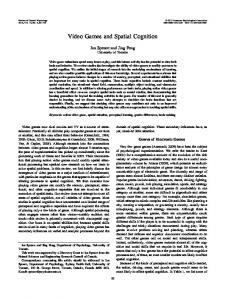
to the end of the opposite arm. As a result, rats had to unlearn what they had previously learned. During the testing phase of the task, an 8-arm probe was introduced every third trial, enabling O’Keefe to evaluate the rats’ orientation during remapping. For lesioned animals the results indicated that in the T-maze there was an abrupt shift from the incorrect to the correct reward arm, but in the 8-arm radial maze the shift in the rats’ orientation was incremental from the left starting quadrant (-90°, -45°) through straight ahead (0°) and into the new right reversal quadrant (+45°, +90°). The conclusion about lesioned rats’ behavior was that the choice in the T-maze was based on the goal location relative to their body. On the other hand, the performance of normal rats in the T-maze proceeded in the same way as in lesioned rats, but in the 8-arm radial mazetheir orientation did not shift in a smooth manner but jumped around randomly. O’Keefe concluded that the reversal performance of normal rats was not based only on their orientation system, but also on the use of the hippocampal cognitive mapping system that in this case was based on the maze shape. In this experiment, rats with hippocampal lesions learned the procedure to reach the reward location, a process that is attributed to the striatum (Schultz et. al, 1998), whereas normal rats employed their hippocampus to build a spatial representation based on the maze shape due to the absence of other visual cues. II. A BIOLOGICALLY-INSPIRED M ODEL OF SPATIAL COGNITION IN RATS The model of spatial cognitioncomprises distinct functional modules shown in Figure 2 that capture some properties of rat brain structures involved in learning and memory. In this section, we provide the biological framework underlying our computational model, as well as the detailed description of all its modules. Figure 2. The modules of the spatial cognition model and their interaction. r= immediate reward; PI= kinesthetic information pattern; LP= landmarks information pattern; AF= affordances perceptual schema; PC= place information pattern; rˆ = effective reinforcement; EX= expectations of maximum reward over a sequence of nodes and their corresponding directions (DX); DIR= next rat direction; ROT= rat rotation; DIS= next rat moving displacement.

A. Biological Background The biological framework of the proposed model is illustrated by Figure 3. Figure 3. The biological framework underlying the computational spatial cognition model. Glossary: LH – Lateral Hypothalamus; RC – Retrosplenial Cortex; EC – Entorhinal Cortex; VTA – Ventral Tegmental Area; VS – Ventral Striatum; NA – Nucleus Accumbens; PLC – Prelimbic Cortex. Inputs/Outputs: r= primary reinforcement; sr= secondary reinforcement; rˆ = effective reinforcement; DR= dynamic remapping perceptual schema; LPS= landmark perceptual schema; AF= affordances perceptual schema; PI= kinesthetic information pattern;

p. 4

LP= landmarks information pattern; PC= place information pattern; EX= expectations of maximum reward and their corresponding directions (DX); DIR= next rat direction; ROT= rat rotation; DIS= next rat moving displacement.

The hypothalamus is considered as the main area where information related to the rat’s internal state is combined with incentives (Risold et al., 1997). Specifically, food seeking and food intake are thought to be under control of the lateral hypothalamus (Kelley, 2004). Therefore, the motivation module of the model is functionally related to this brain area, which computes the value of the rat’s hunger drive and produces the immediate or primary reward the animal gets by the presence of food (r). The posterior parietal cortex (PPC) is assumed as a sensory structure receiving multimodal information such as kinesthetic, visual and relative to affordances. It has been suggested that PPC is part of a neural network mediating path integration (Parron and Save, 2004), where the retrosplenial cortex (RC) is also involved (Cooper and Mizumori, 1999; Cho and Sharp, 2001). Thus, we attribute to PPC the representation of the updated position of the rat’s point of departure each time the animal moves in relation to its current position by means of a dynamic remapping perceptual schema (DR), and to RC, the generation of kinesthetic information patterns (PI) carried out by the path integration feature detector layer in our model. The hippocampus reinitializes the anchor position in DR when necessary (e.g., at the beginning of a trail in a given experiment). We made the assumption that the entorhinal cortex (EC) is involved in the landmarks processing.In this way, EC receives spatial information about landmarks from PPC (Redish, 1997), i.e. distance and relative orientation of each landmark encoded in a landmark perceptual schema (LPS), and then, landmarks information patterns are produced and integrated in a single pattern representing the egocentric view from the animal (LP). It has been suggested that, preceding the rat’s motion, nearly half of the cells in PPC exhibit movement-related activity discriminating among basic modes of locomotion: left turns, right turns, and forward motion (McNaughton et al., 1994). Therefore, we attribute to PPC the generation of the affordances perceptual schema (AF) encoding possible turns the rat can perform at any given time being at a specific location oriented to a certain direction. The place representation module of our model comprises a place cell layer (PCL) and a world graph layer (WGL). The hippocampus receives kinesthetic and visual information from RC and EC respectively. The activity of place cells results from the integration of both information sources. Overlapping place fields in the collection of neurons in PCL are associated with a physical area in the rat’s environment that is identified directionally by the ensemble activity pattern (PC), and whose extension is determined by affordances changes sensed by the animal during exploration. It should be pointed out that we are


not modeling the distinction between the ensemble dynamics of hippocampal regions CA3 and CA1 (Guzowski et al., 2004). Associations between overlapping place fields and physical areas are represented in the model by WGL through a holistic or global spatial map. Besides the mapping process, WGL performs place recognition. We have analyzed two hypothes es related to the situation of WGL within the rat’s brain: (i) the hippocampus, since according to (Hollup et al., 2001(1)), hippocampal lesions caused a severe but selective deficit in the identification of a location, suggesting that the hippocampus may be essential for place recognition during spatial navigation; and (ii) the prelimbic cortex, a subregion of the rat frontal cortex, which is involved not only in working memory, but also in a wide range of processes that are required for solving difficult cognitive problems (Granon and Poucet, 2000), and in the control of goal-directed behaviors (Grace et al., 2007). As our model relies on the exploitation of the spatial map maintained in WGL to enable goal-oriented navigation, we preferred to assume that the functionality of WGL could be corresponded to the prelimbic cortex. Reward information is processed in the basal ganglia by its dopaminergic neurons, which respond to primary and secondary rewards, and their responses can reflect “errors” in the prediction of rewards, thus constituting teaching signals for reinforcement learning. Neurons in the ventral striatum (nucleus accumbens) are activated when animals expect predicted rewards, and adapt expectation activity to new reward situations (Schultz et. al, 1998). Houk et al. (1995) proposed that the striatum implements an Actor-Critic architecture (Barto, 1995), in which an Adaptive Critic predicts reward values of any given place (PC) in the environment and produces the error signal ( rˆ ). A number of Actor units are included in this learning architecture representing possible actions to be performed by the rat. In our model, Actor units correspond to possible rat’s orientations being at any given place. Reward expectations associated to these orientations are adapted by means of rˆ . Recently, it has been suggested that rats with lesions of the hippocampal dentate gyrus (DG) are severely impaired in reinforced working memory tasks, and that the performance during these tasks is strongly correlated with cell density in DG but not with cell density in the CA1 and CA3 areas (Hernandez-Rabaza, et al., 2007). Thus, since those rats were specifically impaired in their ability to update spatial information essential to guide goal-oriented behaviors, we suppose that Actor units could be located in DG. In this way, we suggest that the striatum should influence the hippocampus through DG by sending the expectations of future reward corresponding to the animal’s actions that are exploited by DG to allow the appropriate performance of the animal during reinforced spatial tasks. Finally, the action selection module of the model determines its motor outputs consisting on the next direction of the rat’s head, the required rotation to point to that direction, and the

p. 5

moving displacement. B. Affordances Processing The notion of affordances for movement, adopted from (Gibson, 1966), represents all possible motor actions that a rat can execute through the immediate sensing of its environment; e.g., visual sighting of a corridor – go straight ahead, sensed branches in a maze – turn. In our model, affordances for movement are coded by a linear array of cells called affordances perceptual schema (AF) representing possible turns from -180o to +180o in 45o intervals , which are relative to the rat’s head. Each affordance is represented as a Gaussian distribution in AF, where the activation level of neuron i is computed as follows :

AFi = h e

− (i − a ) 2 2d 2

,

(1)

where d is the width (variance) of the Gaussian, h is its height, and a is its medium position that depends on the particular affordance. Specifically, we employ a=4+9m with m an integer value between 0 and 8 corresponding to an affordance between -180° and +180° in 45° intervals. There is a Gaussian in AF representing each available affordance at any given time. For example, a rat orie nted to north and located at the junction of the T-maze shown in Figure 1(a), senses the following affordances: -90°, +90° and +/-180°, i.e., the rat can turn 90° to the left, 90° to the right or return, and the perceptual schema AF generated by the model would have the form illustrated in Figure 4(a). In other case, a rat located at thecenter of the 8-arm radial maze shown in Figure 1(b), perceives eight affordances (0°, +/-45°, +/-90°, +/ -135° and +/ -180°), i.e., the rat can move ahead, turn 45°, 90° or 135° to the right or left, or return. Figure 4(b) illustrates the representation of these eight affordances by the array AF. In the work by (Guazzelli et al., 1998), affordances are also encoded as Gaussian distributions within a perceptual schema, and additionally, this perceptual schema is processed to produce affordances states representing different motor situations experienced by the animal within the environment. Then, specific affordances are reinforced in these states thus contributing to determine the simulated rat’s decisions when experiencing particular motor situations. However, since the model by Guazzelli et al. assumes that the rat will experiment only different motor situations while exploring an environment, it fails when the animal executes the same reinforced affordance being at the same affordances state in two different contexts. Figure 4. (a) The affordances perceptual schema AF generated by the affordances processing module of the model when the rat is oriented to north in the junction of a T-maze. (b) The perceptual schema AF generated when the rat is at the center of an 8-arm radial maze. The medium position a of each Gaussian in any AF is indicated in the figure together with the integer value m used to compute a in equation (1).


C. Motivation In the model, the animal’s motivation is related to its need to eat: the hunger drive. According to (Arbib and Lieblich, 1977), drives can be appetitive or aversive. The Fixed Critic (FC) module of the model computes the hunger drive D in time t+1 using (2), and the immediate reward or primary reinforcement r the animal gets by the presence of food using (3). The reward depends on the rat’s current motivational state. If it is extremely hungry, the presence of food might be very rewarding, but if not, it will be less rewarding. D(t + 1) = D(t ) + α d d max − D(t ) − a D( t ) + b d max − D (t ) (2) (3) r (t ) = D (t ) / d max Each appetitive drive spontaneously increases with every time step towards dmax (constant value), while aversive drives are reduced towards 0, both according to a factor a d (constant value) intrinsic to the animal. An additional increase occurs if an incentive b is present such as the sight or smell of food. Drive reduction a takes place after food ingestion. D. Path Integration Kinesthetic information refers to internal body signals generated during rat’s locomotion. These signals are used by rats to carry out the path integration process, by which they update the position of their point of departure (the environmental anchor) each time they move in relation to their current position. In this way, path integration allows the animal to return home (Mittelstaedt and Mittelstaedt, 1982; Etienne, 2004). At any time step t, kinesthetic information injected to the path integration module of the model includes the magnitude of the rotation and translation performed by the animal at t-1. This module is composed of a dynamic remapping layer (DRL), and a path integration feature detector layer (PIFDL). DRL represents the anchor position in the rat’s environment by a two-dimensional array of neurons called dynamic remapping perceptual schema (DR). The use of dynamic remapping related to path integration wasoriginally conceived by (Dominey and Arbib, 1982), and implemented by (Guazzelli et al., 1998) inspired in their prior model. The anchor position is codified as a Gaussian distribution in DR, where the activation level of neuron i, j is computed according to (4):

DRi , j = h e

−(i − y) 2 − ( j − x )2 + 2d 2 2d 2

,

(4)

where d is the width of the Gaussian, h is its height, and x, y codify the anchor initial coordin ates in a plane representing a particular environment. The anchor position (i.e., the Gaussian curve) is displaced in DR each time the rat moves by the same magnitude but in opposite direction to the rat’s movement, simulating in this way how the anchor mo ves away from the rat as the rat moves forward in its environment. Figure 5(a) shows an example , step

p. 6

by step, of a rat exploring a T-maze from the base of the T (labeled as “O”) to the end of the right arm of the T (labeled as “E”). Figure 5(b) presents a top-view of DR illustrating the displacement of the position of the rat’s point of departure each time the rat moves. When the rat begins the exploration at “O”, DR presents the anchor position at initial coordinates (2, 4). While the rat is oriented to north and moves step by step along the vertical corridor of the T until the junction location, the anchor position is displaced in DR row by row in direction south (from coordinates (2, 4) to (5, 4)). Then, the rat turns right at the junction of the T orienting itself to east, and moves step by step until the end of the right corridor. Thus, the anchor position in DR is displaced column by column in direction west from coordinates (5, 4) to (5, 2). Figure 5. (a) An example of a rat exploring a T -maze step by step from location labeled as “O” to location labeled as “E”. (b) A simplified top -view of a dynamic remapping perceptual schema (DR) representing the displacement of the anchor p osition from coordinates (2, 4) to (5, 2) each time the rat moves by the same magnitude but in opposite direction. Filled circles represent the top-view of the peak of the Gaussian curve in DR.

DRL updates the anchor position in DR by applying a convolution operation between DR and the “mask” M, which is a two -dimensional array used to encode the opposite direction of the rat’s head. The convolution operation is stored in a two-dimensional array C with the same dimensions of DR, and the computation of every element k, l is described in (5): n

Ck ,l =

n

2

2

   M p + n , q + n × DRk − p , l − q  ,  2 2  p= − n q= − n

∑ ∑ 2

(5)

2

where n is the dimension of M. Then, DR is updated according to C by centering the medium position of the Gaussian at the coordinates (r, c) of the maximum value stored in C. Thus, the activation level of every neuron i, j in DR is recomputed according to (6): DRi , j = h

− (i − r ) 2 − ( j − c ) 2 + 2 2 2d e 2d

Cr , c = max( Ck , l ) ∀ k , l .

(6)

In this path integration module, the DRL layer is connected through the DR schema to the PIFDL layer. Figure 6 illustrates the architecture of the module. In our basic model, every neuron in DR is randomly connected to 50% of the neurons in PIFDL. Nevertheless, as a future extension to the model, this high projection level will be adjusted to the one known or hypothesized by neuroscientists between the posterior parietal cortex and the retrosplenial cortex. Connection weights between layers are randomly initialized and normalized between 0 and 1 according to (7): w ij wij = , (7) w ij

∑ i


where w ij is the connection weight between a neuron i in DR and a neuron j in PIFDL. Figure 6. The path integration module of the spatial cognit ion model. DRL stands for dynamic remapping layer. PIFDL stands for path integration feature detector layer. Connection weights w between the dynamic remapping perceptual schema DR and PIFDL are updated through Hebbian learning. The activation values A of neurons j in PIFDL are organized in neighborhoods of m cells each one. New activation values G are assigned to neurons within neighborhoods. These values are stored in the linear array PI representing a kinesthetic information pattern produced by the module.

The activation level Aj of neuron j in PIFDL is computed by adding the products between each input value Ii coming from neuron i in DR and the corresponding connection weightw ij as follows:

A j = ∑ I i wij .

(8)

i

Synaptic efficacy between DRL and PIFDL is updated by Hebbian learning (Hebb, 1949) in order to ensure that the next time the same or similar activation pattern is presented in DRL, the same set of units in PIFDL is activated representing a kinesthetic information pattern. In fact, we also employ the Hebbian learning rule in the landmarks processing and the place representation modules of the model to enable the generation of visual information patterns and the posterior recognition of places. The application of the Hebb rule is inspired on the original model by (Guazzelli et al., 1998). It involves the division of the population of N neurons in PIFDL in a number of neighborhoods with an equal number m of cells, where m w na

and DX na + 2 = 180° ) and the corresponding expectations of reward

, (16)

dc dc EX na + 2 = w na + 2 ; DX na + 2 = dc dc d1 d8 dc db wna + 2 = max( wna + 2 ,K , wna + 2 ) ∧ wna + 2 > w na +1 da , db , dc where EX na EX na +1 EX na + 2 are the expectation of reward

values selected from map nodes na, na+1, na+2 in directions

where N is the total amount of activation values in PC. AC uses predictions computed at times t and t-1 to determine the secondary reinforcement, discounting the current prediction at a rate ? to get its present value. The addition of the secondary reinforcement with the primary reinforcement r computed by the Fixed Critic module constitutes the effective reinforcement rˆ as described by (18): rˆ(t ) = r( t) + γ P (t) − P(t − 1) . (18) The effective reinforcement is considered to update the connection weights w between PCL and AC, and also between

db dc da, db, dc; wda na , wna +1 , wna + 2 are connection weights

p. 9


Actor units and map nodes. In the first case we used wi (t + 1) = wi (t) + β rˆ( t) ei (t ) ,

(19)

where ß is the learning rate. In the second case we used

wdk (t + 1) = w dk (t ) + β rˆ(t )edk (t ) ∀ node k, actor d , where wkd (t

(20)

+ 1) is the connection weight between node k and

the Actor unit corresponding to direction d at time t+1, and

ekd (t ) is the eligibility trace of Actor unit d in node k at time t. As shown in (19) and (20), both learning rules depend on the eligibility of the connections. At the beginning of any trial in a given experiment, eligibility traces in AC and in Actor units are initialized to 0. At each time step t in a trial, eligibility traces in AC are increased in the connections between PU and the most active neuron within each neighborhood in PCL. If the action executed by the rat at time t-1 allowed it to perceive the goal, then eligibility traces are increased more than in the opposite case. The eligibility trace e of every connection i at time t is updated as shown in (21): (21) ei (t ) = e i (t −1) + χPC i (t ) PC i (t ) = 1, where ? is the increment parameter, and PC is the linear array produced by PCL storing the activation values between 0 and 1 of its neurons. Also at time step t, the eligibility trace of the connection between the active node na in the map and the Actor unit corresponding to the current rat’s direction dir is increased by t as described by (22): dir e dir na (t ) = e na (t − 1) +τ .

(22)

Finally, after updating the connection weights between PCL and AC, and between Actor units and map nodes at any time step t in the trial, all eligibilities decay at a certain rate ? as shown in (23): (23) ei (t ) = λei (t − 1) . H. Action Selection At a given location, the choice of the rat to turn to a specific direction at any given time t is determined in our model by the action selection module (SS) by means of four signals corresponding to: (i) available affordances at time t (AF), (ii) a random rotation between possible affordances at time t (RPS), (iii) rotations that have not been explored from the current rat’s location (CPS), and (iv) the global exp ectation of maximum reward (EMR). These signals are represented in linear arrays referred to as perceptual schemas by means of one or more Gaussians, whose medium positions within the array correspond to specific relative rotations between -180° and +180° in 45° intervals. The AF perceptual schema is generated by the affordances processing module in the model. In this case, there are as many Gaussians in the schema as possible turns the rat can execute at any given time. Each Gaussian is centered at the array

position corresponding to the specific relative rotation. The RPS perceptual schema presents just one Gaussian centered at a random array position between the positions corresponding to possible affordances at the given time. The CPS perceptual schema represents the animal’s curiosity at any given location to execute rotations that lead to places not yet represented in the topological map. Therefore, this schema presents as many Gaussians as unexecuted rotations at the given location within possible affordances at the given time. Each Gaussian is centered at the array position corresponding to the unexecuted rotation. To build EMR, SS uses the expectation of reward values EX and the corresponding directions DX selected by WGL over the sequence of nodes in the map from the active node. As we described in Section II.F, there can be at most three different directions and expectation of reward values associated to three nodes in the sequence. Each k expectation of reward value EX k is represented as a Gaussian in EMR; thus, t here can be at most three Gaussians. The medium position of each Gaussian in the array corresponds to t he rotation the rat has to execute to orient to the k direction DX k , and its height depends on EX k . In this way, EMR is initialized as follows:

 −( i −M k ) 2     EX k e 2d 2  , (24) EMRi =  max( EX )  k     where d is the width of the Gaussian, max is a function that determines the biggest expectation of reward value between all values EX, and M k corresponds to the medium position of

∑

the Gaussian for EX k . M k is determined as 4+9m with m an integer value between 0 and 8 corresponding to the specific rotation between -180° and +180° in 45° intervals that the rat has to execute to orient to DX k . Figure 12(a) illustrates the initialization of EMR considering the case of the map of a T-maze presented in Figure 10 and the values EX and DX selected by WGL. In order to generate a global expectation of reinforcement signal that will influence the next behavior of the rat, the “center of mass” c is computed over EMR, considering just the activation values of neurons in EMR located in the medium position of different Gaussians. The computation of the center of mass is described by (25):

∑(

(

))

 EMRi × i − nPS 2   i  + nPS , (25) c = int 2   EMRi   i   where c corresponds to the position of the center of mass in EMR, EMRi is the activation value of the neuron located in

∑

the array at the medium position i of an existing Gaussian in EMR, nPS is the total amount of neurons in the perceptual schema EMR, and int is a function that determines the integer

p. 10


value of its argument. Then, EMR is updated to represent the global expectation of reward signal by means of just one Gaussian centered at c with height corresponding to the addition of the heights of every k existing Gaussian as follows: −( i −c) 2

 EX k  2 d 2 . (26) EMRi =  e  max( EX )   k  If there is no available affordance coinciding with the center of mass over EMR, this center is moved in the array to the position that corresponds to the relative rotation that orients the rat to direction DX na selected from the active map node

∑

na (the first node in the sequence analyzed by WGL). Figure 12(b, c) illustrates the determination of the center of mass for the example provided in Figure 10 and the update applied to EMR. Figure 12. An example of t he generation of the global expectation of maximum reward perceptual schema (EMR) carried out by the action selection module of the spatial cognition model. (a) Considering the ° 90° ° expectation of reward values EX 90 , and EX 180 na = 1 EX na +1 = 2 na + 2 = 3 in directions DX na = 90° , DX na+1 = 90° and DX na +2 = 180° selected by WGL in t he map presented in Figure 10 when the rat is oriented to 90° and located at the base of the T-maze, EMR is initialized with two Gaussians, one for each different direction DX. Gaussian 90° with height 1 is centered at position 40 in EMR corresponding to relative rotation 0°, while Gaussian 180° also with height 1 is centered at position 22 corresponding to relative rotation -90°. (b) EMR is updated to present just one Gaussian distribution with height 2 and medium position 31 resultant from the computation of the “center of mass” using equation (25). (c) Although relative rotation -45° (position 31 in EMR) anticipates the target direction 135° from the rat location (since the food reward is placed at the end of the left arm of the T), this is not a possible affordance from there, thus the medium position of the Gaussian is moved to position 40 corresponding to rotation 0° and direction DX na = 90° .

Finally, the action selection module adds, neuron by neuron, the activation values stored in perceptual schemas AF, RPS, CPS and EMR producing a new perceptual schema S, where the activation value of any neuron i is computed as described by (27): (27) Si = AFi + RPSi + CPSi + EMRi . The influence of each signal in S depends on the height of its Gaussians. Specifically, the significance order of the signals in the selection of the next rat action is the following: (i) EMR, (ii) AF, (iii) CPS, and (iv) RPS. Figure 13 illustrates the generation of S. In the resultant array S, SS considers the position of the neuron with the highest activation value in order to determine the next direction of the rat’s head DIR, from 0° to 315° in 45° intervals , and the required rotation ROT to point to this direction. If DIR is different from the current direction, the next rat’s moving displacement DIS is 0, giving the animal the opportunity to perceive a different view from the same place.

Otherwise, DIS is 1, corresponding to a “motion step” in direction DIR. Figure 13. An example of the generation of the perceptual schema S used by the action selection module to determine the next rat’s direction DIR, the required rotation ROT and the next moving displacement DIS, considering the case presented in Figure 10. (a) The affordances perceptual schema (AF) produced by the model when the rat is oriented to 90° and located at the base of a T -maze (the rat can just move ahead) . (b) The random perceptual schema (RPS) showing a Gaussian centered at the position corresponding to the only existing affordance. (c) The empty curiosity perceptual schema (CPS) since there are not possible turns unexecuted by the rat from its location. (d) The global expectation of maximum reward perceptual schema (EMR) created in Figure 12. (e) The perceptual schema S resultant from the addition of perceptual schemas shown in (a), (b), (c) and (d). According to S, ROT is 0° (i.e., no rotation is needed to orient the rat to the next direction), DIR is 90°, and DIS is one “motion step” since DIR is the same as the current rat’s direction.

In the model by (Guazzelli et al., 1998), the action selection process considers the addition of reward expectations derived from their TAM model with reward expectations from their WG model. However, as reward expectations from TAM were computed over the assumption of having different motor situations or affordances states in the environment, the simulated rat fails to find the goal when the maze includes two or more decision points offering the same affordances state. In our model, after having finished a training trial in a given experiment, the rat return s to its departure point, and SS computes the next rat’s direction DIR from the built map. Since the rat marks as visited the arcs connecting the path of nodes followed during the trial, SS uses the opposite directions of these arcs to compute DIR during the return process. The rat deletes those arc marks while returning to the departure location. To enable goal-directed navigation, different from (Guazzelli et al., 1998), SS implements a backwards reinforcement over the nodes in the path followed by the rat. The eligibility traces of the Actor units are updated in the direction of the arcs connecting the nodes in the path. Each eligibility trace is updated in a given amount of reinforcement divided by the amount of steps the rat performed to move from one node to the next one in the path. If the animal found the goal at the end of the path, the update is positive; otherwise, it is negative. The reinforcement is initialized to a certain amount at the beginning of any trial in the experiment, and this amount decreases as the distance from a node to the goal or to the end of the path increases . The backwards reinforcement process is carried out during the return to the point of departure. Specifically, the algorithm followed by SS during the return process and the backwards reinforcement at each step of the rat is presented in Table 1. It should be pointed out that the return process is not a necessary condition for maintaining eligibility traces during the learning process. In fact, we implement the return process

p. 11


just to execute the experiments in an autonomous manner. Figure 14 illustrates both, return and backwards reinforcement processes, considering again the case of a rat exploring a T-maze from the base of the T to the end of the reward left corridor. T ABLE 1. T HE ALGORITHM FOLLOWED BY THE ACTION SELECTION MODULE OF THE MODEL DURING THE RETURN PROCESS OF THE RAT AT THE END OF ANY GIVEN EXPERIMENT’ S TRIAL .

If the return process begins, then Remember the node in the map linked to the active one through the arc marked as visited Delete the mark in the arc Compute the next direction of the rat as the opposite of the arc Else if the return process is not beginning, then If affordances did not change from time t-1 to t, then Make the next direction of the rat equal to its direction in time t Else Update t he active node as the node pointing to it through the arc marked as visited Divide the amount of reinforcement (R) by the amount of rat steps associated to the arc of th e active node marked as visited If the goal was reached by the rat at the end of the experiment’s trial, then Add R to the eligibility trace of the Actor unit corresponding to the direction of the arc marked as visited in the active node Else Subtract R from the eligibility trace of the Actor unit corresponding to the direction of the arc marked as visited in the active node Diminish R If there is an arc marked as visited pointing to the active node in the map, then Remember the node linked to the active one through this arc Delete the mark in the arc Compute the next direction as the opposite of the arc

T ABLE 2. M AIN PARAMETER VALUES USED IN THE IMPLEMENTATION OF THE SPATIAL COGNITION MODEL . Paramete Description Value r nPS Amount of neurons in any linear perceptual 80 schema d Variance of any Gaussian distribution 3 N

Amount of neurons in any feature de tector layer (i.e., PIFDL, LFDL, LL, PCL)

400

nN

Amount of neighborhoods within a feature detector layer (i.e., PIFDL, LFDL, LL, PCL)

5

m

Amount of neighborhood

each

80

h

Height of any Gaussian in the affordances perceptual schema (AF), in any landmark perceptual schema (LPS), and in the dynamic remapping perceptual schema (DRPS) Height of the Gaussian centered at a random position in the random perceptual schema (RPS)

1

hR

0.04

Height of any Gaussian in the curiosity perceptual schema (CPS)

0.05

hE

Height of the Gaussian in the global expectation of maximum reward perceptual schema (EMR) Maximum value of the hunger drive employed by Fixed Critic module Intrinsic factor of hunger employed by Fixed Critic module Reduction of the hunger drive after food ingestion Increase of the hunger drive aft er perceiving an incentive Dimension of mask M employed by DRL to encode the opposite global di rection of the rat’s head Learning rate in any application of the Hebb rule Discount factor used by the Learning module to compute the effective reinforcement

≥1

αd a b n

a

In Table 2 we show the values for the most important parameters used in the equations of the model.

within

hC

d max

Figure 14. An example of the return and backwards reinforcement processes carried out by the action selection module of the model. (a) The rat explores a T -maze from location a to location h where the goal is located. In the corresponding map with five nodes numbered in order of creation, arcs between nodes are associated to the rat’s direction d when it moved from one node to the next one, and with the amount of steps s it took to do that. Besides, arcs in the path followed by the rat are marked as visited with a “v”. (b) The rat returns from location h to location a deleting all marks “v” from the map. In this case, the map shows the opposite directions od computed by the action selection module from arcs in the route followed by the rat. The backwards reinforcement process involves the positive update of eligibilities e in Actor unit 180° of node 4, Actor unit 180° of node 3, Actor unit 90° of node 2, and Actor unit 90° o f node 1. The applied increase is given by the decreasing amount of reinforcements R, R 1, R 2 and R 3 divided by the rat steps 2, 1, 3 and 1 respectively.

neurons

?

20 0.003 0.2 0.15 3

0.001 0.85

ß

Learning rate employed by the Learning module to update connection weights between PCL and AC, and between Actor units and map nodes

0.041

?

Update factor applied by the Learning module to eligibility traces of connections between PCL and AC Update factor applied by the Learning module to the eligibility trace of the connection between the active map node and the Actor unit in the rat’s direction Decay factor applied by the Learning module to all eligibility traces

0.3

t

?

0.1

0.8

III. EXPERIMENTAL RESULTS The rat cognitive model was designed and implemented

p. 12


using the NSL system (Weitzenfeld et al., 2002). The model can interact with a virtual or real robotic environment through an external visual processing module that takes as input the image perceived by the robot, and a motor control module that executes rotations and/or translations on the robot. The model runs online and in real time, using a Sony AIBO ERS-210 4-legged robot and a 1.8 GHz Pentium 4 PC, which communicates with the robot wirelessly. As sensory capabilities, we only use the local 2D vision system of the robot, whose view field covers about 50° in the horizontal plane and 40° in the vertical plane. Using its local camera, the robot takes at each step three non-overlapping snapshots (0°, +90°, -90°) to obtain 45° affordance intervals. The external visual processing module analyzes the images to compute the amount of pixels of every relevant color, and determine the possible presence of the goal and landmarks. In this way, considering the known and apparent sizes of landmarks in each image, the module estimates the dis tance and relative orientation of each visible landmark from the rat. The amounts of colored pixels are used also by the affordances processing module to determine possible rotations the robot can execute from its current location and build the affordances perceptual schema. The external motor control module, on the other hand, receives the magnitude of the next robot’s rotation and displacement from the action selection schema of the model, and interacts remotely with the AIBO robot motor interface to perform rotation and translation operations. A number of experiments were performed to test the bio-inspired model in providing a robot with spatial cognition and goal-oriented navigation capabilities in simplified environments with controlled illumination. Specifically, we employed a T-maze, an 8-arm radial maze, a multiple T-maze, and a maze surrounded by landmarks. In all cases, colored papers pasted over the walls inside the mazes were used just to compute affordances, since we have exploited only the robot head camera to detect obstacles in our experiments. The experiment carried out in the T-maze and in the 8-arm radial maze is inspired on the reversal task implemented by O’Keefe (1983), which we performed in both mazes separately, and then we extended it within a multiple T-maze. On the other hand, the behavioral procedure that we tested in the maze surrounded by landmarks is inspired on the Morris experiment (Morris, 1981) adapted to a land-based maze with corridors. In fact, a land-based version of the M orris task was previously implemented by Hollup et al. (2001(2)) to determine that hippocampal place fields in a land-based maze with a circular corridor placed at its center are largely controlled by the same factors as in the open water maze and in the water maze restricted by a corridor in spite of differences in kinesthetic input. As kinesthetic input to the model is not provided by an odometer that computes both linear and angular

displacements of the robot, the self-movement signals are traced by the external motor control module of the model and sent directly to the path integration module . To do this, all mazes were discretized by a 25 x 25 matrix constituting the dynamic perceptual schema (DR), where the coordinates of the robot’s point of departure as well as its initial direction are predetermined. Each time step, when the motor control module performs rotation and translation commands, it sends this information to the dynamic remapping layer of the model in order to update the anchor position in DR accordingly. Additionally, the motor control module updates the current direction of the robot by considering the rotation command just executed, and sends the new direction to the affordances processing module, as well as to the landmarks processing module in order to work properly. The following sections describe the robotic experimentation results obtained in the different mazes. A. Experiment I: T-Maze In the T-maze shown in Figure 15(a), the robot navigates from the base of the T to either one of the two arm extremes, and then it returns to its departure location. This process is repeated in every experiment’s trial. We should point out that the autonomous return is not part of the protocol originally implemented by O’Keefe during the reversal task. In fact, at the end of any given trial, rats were manually placed again at the base of the T. Nevertheless, we decided to carry out the return process in order to execute the complete experiment without human intervention, except to change the goal location at the beginning of tests. During the training phase, the goal is placed in the left arm of the maze. The system allows the robot to recognize the goal just one step away from it in order to prevent a taxon or guidance navigation strategy. At the beginning o f training, the decisions of the robot at the T-junction are determined by the curiosity for unexecuted rotations, and by noise, which is represented as a random rotation by the action selection module. After having visited each arm once, the curiosity level for rotating to -90° and +90° at the choice point decreases, thus prevailing noise. Then, the robot turns left or right randomly, and eventually it meets the criterion once the expectation of finding reward in orienting to 180° at the choice point becomes bigger than noise. When this event occurs, the training phase ends. The robot performs as many trials as necessary to learn to go to the left arm to get the reward . The average duration of the training phase in terms of the number of trials was 12, which was obtained from executing the model six times. Considering that a trial lasted 2 minutes in average, the training phase was completed by the robot in a little more than 20 minutes. When the testing phase begins, the goal is moved to the right arm. This situation constitutes , in the words by O’Keefe, “a discrimination reversal problem that involves an unlearning process giving up a previously correct hypothesis and

p. 13


switching to a new one” (O’Keefe and Nadel, 1978). Superficially, this switch might seem quite easy to accomplish, in that the same two options remain relevant in the reversal task. Thus, overtraining on the initial task often has the effect of facilitating reversal. However, this effect is rarely seen in spatial tasks with rodents; in fact, the opposite happens. According to O’Keefe, most spatial tasks are initially solved by normal animals using place hypotheses , i.e. learning reward locations, but overtraining causes a shift towards the use of orientation hypotheses , i.e. learning the procedure to reach the goal from the departure location (O’Keefe and Nadel, 1978). During reversal, the expectation of future reward for the left arm decreases continuously each time the robot reaches the end of that arm not finding reward, since this event is coded as frustrating by the reinforcement learning rule. When the expectation of reward becomes smaller than noise, the robot starts visiting the right arm, thus increasing the expectation of reward for this arm. Since in the beginning the expectation value is smaller than noise, the robot tends to choose any arm randomly until it meets the criterion when the expectation of reward for turning right at the choice point is bigger that noise. The average performance of the robot during reversal derived from six executions of the model is shown in Figure 16(a), where the robot’s behavior is expressed in terms of percentage of correct choices at the T-junction. As a result from training, 100% of the robot’s choices were correct (control). The graph shows 32 testing trials. As can be seen, the robot takes 12 trials to unlearn the previously correct hypothesis (criterion). From trial 13, it has learnt the new one. In this way, the percentage of correct choices shifts from 36% in trial 12 to 95% in trial 16 and 100% from there. Comparing our results with those reported by O’Keefe with normal rats in (O’Keefe, 1983), we can appreciate a behavioral similitude with the robot in the T-maze. O’Keefe presented the average results obtained from four rats. His graph also shows 32 testing trials and a control measure of 100% of correct choices at the T-junction after training. In this case, rats reached the criterion in trial 20, where the percentage of correct choices was between 20% and 40%. By trial 24, rats chose the new reward arm in more than 90% of the times until performing 100% of correct decisions. In Figure 16(a) and in the graph reported by O’Keefe in (O’Keefe, 1983), as described by him, there is an abrupt change from the incorrect to the correct arm. During the experiment, the robot builds and maintains the

topological-metric spatial representation shown in Figure 15(b). In this task, the ensemble activity of the neurons found in the place cell layer of the model was determined only by the use of kinesthetic information, since no landmarks were available. Figure 15(c) illustrates a sample of the ensemble activity registered from the place cell layer when the robot reaches the T-junction indicated as location “e” in Figure 15(a) being oriented to 90°. Although 25% of place cells showed receptive fields to some extent at this location, we are showing only the five most active neurons from each neighborhood within the layer. Overlapping place fields of the 25% of cells are mapped to node 3 in the spatial representation, where the activity pattern of the collection of place cells is stored in an Actor unit associated with direction 90°. Different from what occurs with rats, place cells in our model respond directionally; i.e., when the robot turns left at the T-junction, other group of neurons responds. In this situation, the current ensemble activity is stored in a new Actor unit associated with direction 180° and connected to the same node 3. The relevance of locations in a maze relies on the presence of a reward or on affordances changes sensed by the robot during exploration. In Figure 15(a), for example, the robot considers locations “a”, “b”, “e”, “f”, “g”, “h” and “i” as relevant, and that is why the map includes seven nodes. When the robot reaches location “b” in dire ction 90°, the current ensemble activity of the place cell layer is stored in node 2, and although the activity pattern could slightly vary at locations “c” and “d”, the affordances sensed by the robot did not change from “b” to “c” or “d”, thus activity patterns registered in these locations are averaged and stored in the same node 2, defining in this way its physical extension. After finishing any given trial, the robot returns to the departure location by reading the directions stored in the map and not by random choices, thus the map is not modified with new arcs during this procedure. The return process followed by the robot in this T-maze was documented preliminary in (Barrera and Weitzenfeld, 2006). Finally, it should be pointed out that, different from rats, the robot was programmed to avoid 180° rotations when there exist other possible rotations (0°, +90°, -90°), thus optimizing the exploration process to find the goal. For these reason, arc directions between nodes in the map are one way.

Figure 15. (a) The physical T maze used in the reversal task. Different locations are labeled with letters. The AIBO robot is located at the starting position. (b) The map built by the robot during training. Nodes are numbered in order of creation, and arcs are associated to the robot’s direction when it moved from one node to the next one. (c) A sample of the ensemble activity of place cells when the robot reaches the T -junction being oriented to 90°. The figure shows only the firing rate of the five most active neurons (pc1, pc2, pc3, pc4, pc5) from each neighborhood (n1, n2, n3, n4, n5) within the layer of place cells. decisions in the radial maze also averaged over periods of four trials. T o compare these results with those obtained by O’Keefe with four normal Figure 16. The performance of six robots during the reversal task. Each rats, refer to (O’Keefe, 1983). In our graphs, as in O’Keefe’s, the abrupt graph was obtained by averaging the graphs of the individual robots. T he shift from turning left to turning right in the T-maze reveals the graph in (a) shows the percentage of correct choices in the T -maze averaged over periods of four trials. The graph in (b) presents robot

p. 14


moment (criterion) when the average orientation crosses the midline in the radial maze.

B. Experiment II: 8 -Arm Radial Maze In any given trial of the task in the 8-arm radial maze , the robot departs from the location shown in Figure 17(a), navigates to any other arm extreme, and returns to the departure point. Figure 17(b) presents the map built by the robot during the experiment. Figure 17. (a) The physical 8-arm radial maze used in the reversal task. The picture shows the egocentric directions of the arms in the maze, as well as the AIBO robot at the departure location. (b) The map built by the robot during the experiment. Arcs between nodes are associated to the robot’s direction when it moved from one node to the next one.

The training phase works as in the T-maze with the target placed at the end of the arm relatively oriented to -90°. At the beginning, the decisions of the robot at the choice location when reaching the center of the maze are determined by curiosity and noise. After having visited each arm once, the curiosity level decreases, thus prevailing noise. Eventually, the robot meets the criterion once the expectation of finding reward in orienting to 180° at the choice point becomes bigger than noise. When this event occurs, the training phase ends. The average duration of the training phase obtained from executing the model six times was 13 trials performed by the robot in less than half an hour. During reversal, the expectation of future reward for the -90° arm decreases continuously each time the robot reaches the end of that arm not finding reward. When the expectation of reward becomes smaller than noise, the robot starts visiting other arms randomly. Each time it visits the +90° arm that provides reward, the expectation for this arm increases. The robot meets the criterion when the expectation of reward for turning right at the choice point is bigger that noise. The average performance of the robot during reversal derived from six executions of the model is shown in Figure 16(b), which presents the robot’s choices during 32 trials grouped four by four. As a result from training, the robot chose consistently to turn left at the center location of the maze (control). During reversal, the robot’s orientation did not reveal any systematic shift. As in the T-maze, the criterion occurred around trial 12, when the average orientation crosses the midline of the graph. We also appreciate in our results a similitude with those reported by O’Keefe with four normal rats in the radial maze (O’Keefe, 1983). He also presented a graph showing 32 testing trials , where rats reached the criterion around trial 20. He explained that the abrupt shift from turning left to turning right in the T-maze was revealing the moment when the average orientation crosses the midline in the radial maze. According to our tests, the same fact applies to the robot’s behavior.

C. Experiment III: Multiple T-Maze After completing the reversal task using a T-maze and an 8-arm radial maze, we decided to extend the experiment by considering a more complex maze, where any route to be explored by the robot from a fixed location includes two choice points. To try this, we designed a maze composed of two horizontal Ts based on the arms of one vertical T as shown in Figure 18(a). The work proposed by (Guazzelli et al., 1998) was also validated by replicating the results fromthe O’Keefe’s reversal task in the T-maze and in the radial maze. Nevertheless, the task was implemented within a simulated environment and was hard to extend it to more complex mazes. During any trial of our experiment, the robot navigates from the base of the vertical T to either one of its two arm extremes (0° or 180°) and then to either one of the two arm extremes of the corresponding horizontal T (90° or 270°). Then the robot returns to the departure location autonomously. There are a training phase and a testing phase. In the first one the goal is placed at the end of the right arm (90°) of the left horizontal T (180°), and in the second one, the goal is moved to the end of the right arm (270°) of the right horizontal T (0°). At the beginning of training, the exploration of the maze by the robot is determined by curiosity and noise. The curiosity level for rotating to -90° and +90° at any choice point decreases after having visited each corridor once, thus prevailing noise. The map built during the exploration process is shown in Figure 18(b). At the end of any trial, the backwards reinforcement process takes place over the nodes in map belonging to the path followed by the robot. As described in Section II.H, this process consists on updating the eligibility trace of the Actor units associated to the arc directions between nodes . If the robot reaches the target by the end of the trial, the path is positively reinforced, which can be referred to as route learning; otherwise, the path is negatively reinforced, wh ich can be referred to as route unlearning. Eventually, the robot meets the criterion once the expectation of finding reward in orienting to 180° at the fist choice point and to 90° at the second one becomes bigger than noise. When this event occurs, the training phase ends. The average duration of the training phase obtained from executing the model six times was 13 trials, and considering that a trial lasted 2.5 minutes in average, the training phase was completed by the robot in a few more than 30 minutes. During reversal, the route unlearning process takes place. When the expectation of rewardfor the previously learnt route becomes smaller than noise, the robot starts performing random choices until it meets the criterion once the expectation of reward for orienting to 0° at the fist choice point and to 270° at the second one becomes bigger than noise. When this event occurs, the robot has learnt the new route. The average performance of the robot during reversal derived from six

p. 15


executions of the model is shown in Figure 19, where the robot’s behavior is expressed in terms of percentage of correct decisions at both choice points. As a result from training, 100% of the robot’s choices were correct (control). The graph shows 32 testing trials. The robot takes 12 trials to unlearn the previously correct route to the goal (criterion). According to our expectations, it is possible to appreciate an abrupt shift from the incorrect to the correct route, as occurs in the simple T-maze. In this way, the percentage of correct choices shifts from 32% in trial 12 to 90% in trial 16 and 100% from there. As O’Keefe concluded about normal rats solving the reversal task in the T -maze and in the radial maze, the behavior of the robot in the multiple T-maze relied on the spatial representation built on the bas is of the shape of the maze, since no landmarks were available during the task. Figure 18. (a) The physical extended maze used in the reversal experiment. The goal is presented at the training location. (b) The map built by the robot during exploration . Nodes are numbered in order of creation, and arcs between nodes are associated to the robot’s direction when it moved from one node to the next one. Figure 19. The performance of six robots expressed in terms of percentage of correct decisions during the reversal task in a multiple T-maze. The graph was obtained by averaging the graphs of the individual robots over periods of four trials. An abrupt shift from the incorrect to the correct route can be appreciated.

D. Experime nt IV: Maze Surrounded by Landmarks In the experiment just described in Section III.C, the primary objective was to test the ability of the robot to learn the correct route to the goal from a fixed location by using just kinesthetic information, and to unlearn that route while learning the new one that leads to the target. In the experiment presented in this section, we placed three colored cylinders representing landmarks outside the multiple T-maze in order to test: (i) the place recognition process carried out by the robot employing not only kinesthetic but also visual information while exploring the maze, and (ii) the goal-directed navigation to find the goal from different starting locations. The training phase proceeds as in the previous experiments; i.e., in any trial, the robot starts from a fixed given location, explores the maze until it finds the goal or the end of a corridor, and returns to the departure point. During exploration, the robot builds a map similar to the one shown in Figure 18(b). Before implementing this experiment, we decided to adjust some of the parameters related to the backwards reinforcement process in the model in order to reduce the total duration of the training phase, although rats need several trials to learn the goal location in any maze. As a result , the robot requires just five training trials in average reaching the goal to learn the route from the fixed departure location. We executed the model six times, and the average duration of the training phase was 9 trials , i.e. 23 minutes approximately.

After training, we placed the robot at different departure positions (D1, D2 and D3 in Figure 20(a)) during testing trials. In the best of the six executions of the model, the robot followed direct routes towards the goal as shown in Figure 20(a), and updates the map of the environment as illustrated by Figure 20(b). We should point out that all robots found the goal successfully from all starting positions tested, although some of them took longer paths from locations D2 and D3. The average durations of trials starting at D1, D2 and D3 were 50 seconds, 120 seconds and 140 seconds, respectively. To reach the target from any location, the robot performs place recognition and map exploitation processes. Let’s consider the simplest case starting at location D1 (see Figure 20(a-b)). The robot begins the trial being oriented to 90°. Since no landmarks were visible from there, neurons in the place cell layer of the model respond according to kinesthetic information only. The current ensemble activity of the layer is searched within the nodes in the map and found in Actor unit 270° of node 11. Although the robot’s current direction is not 270°, both activity patterns are similar since none of them encodes for visual information. Thus, node 11 is activated in the map, indicating in this way that the robot recognizes location D1 as previously visited. Then, the robot moves forward and perceives some part of landmark 3 (L3). This time, the current activity pattern of the collection of place cells is not similar to any of those found in the map. This is because the robot had visited that location previously being oriented only to 270° and not to 90°, thus visual information sensed in both directions is different. As a result, the current activity pattern is stored in a new Actor unit 90°, which is associated with the new number 16 node. When the robot reaches the choice point of the corridor, the current ensemble activity of place cells is found within Actor unit 90° of node 9, thus this node is activated. At this location, the expectation of future reward in direction 90° was increased during training in an important manner; therefore, the robot exploits this information when decides to go ahead instead of turning right. From this location, the robot moves forward recognizing the places represented by node 14 in the map until it reaches the target, whose location is represented by node15. The place recognition and map exploitation processes carried out by the robot during trials starting at locations D2 and D3 to reach the goal is similar to the one just described. In these cases , the robot adds nodes 17, 18 and 19 to the map, and employs the reward expectations values to decide to go ahead at location represented by node 3 and turn right at location represented by node 9 when being oriented to 180°. An appropriate comparison between our results and those reported by Morris with normal rats in (Morris, 1981) turns out difficult since we implemented important variations to the original experiment. Nevertheless, as Morris did with normal rats, we could confirm that to find a “hidden” goal in the maze independently of the starting location, the robot requires to

p. 16


exploit its cognitive map by recognizing reward expectations that make it navigate towards the target location successfully. Recently, we tested two different scenarios of this experiment after training the robot: (i) by interchanging landmarks, and (ii) by removing landmarks from the maze (Barrera and Weitzenfeld, 2007). In both situations we could verify that the robot, in real-time, is able to adapt the map previously built during training by adding and/or eliminating nodes in order to reveal changes in the physical configuration of the maze. Figure 20. (a) Routes followed by the robot in three testing trials starting from locations D1, D2 and D3. Landmarks are labeled as L1, L2, L3, and the training departure location as TD. (b) The map updated by the robot during the testing phase. Nodes are numbered in order of creation. Black nodes belong to the route learnt during training.

IV. DISCUSSION AND CONCLUSIONS In this paper we have presented a robotic spatial cognition model that captures some properties of the rat’s brain structures involved in learning and memory. By means of different experiments inspired on classical spatial tasks carried out with rats, we have shown that our model endows the robot, in real-time, with the following abilities: (i) Building of a holistic topological-metric map to represent a maze during exploration. (ii) Learning and unlearning of goal locations through a reinforcement architecture. (iii) Exploitation of the cognitive map to recognize places already visited and to find a target from any given departure location, thus enabling goal-directed navigation. According to the biological background of our model, different from other bio-inspired models, we have suggested how the striatum, related to the rat’s brain reward system, should influence the hippocampus, associated to the spatial representation system, through the dentate gyrus (DG), since it has been discovered recently that during goal-oriented behaviors, rats with lesions of DG are severely impaired in their ability to use the reward expectations associated to spatial locations by the striatum. We have been concerned with testing the proposed robotic system in spatial tasks similar to those carried out with rats, thus obtaining comparable results. Specifically, we reported in this paper a comparison between our results with the robot and those obtained by O’Keefe in 1983 during the classical reversal task. However, since it is difficult to have access to behavioral data derived from many other classical experiments, we are working now on designing and imp lementing new spatial tasks to train and test real rats in order to produce a direct comparison source to be used to evaluate our model in a better manner. From a biological perspective, our basic spatial cognition model will be sophisticated to contribute to experimental

neuroscience by providing a valuable feedback tool to test with robots new hypotheses relative to the underlying mechanisms of the rats’ learning and memory capabilities. In particular, our next goals are to adjust projection levels between the layers of the model according to neuroscientific knowledge, and improve the place representation module by distinguishing between the ensemble dynamics of place cells found in hippocampal regions CA3 and CA1, and by adapting the response of the place cells from unidirectional to multidirectional. From a robotics perspective, many aspects should be addressed before placing our system within a performance scale or comparing it with specific SLAM approaches. Particularly, we need to improve the perceptual system, deal with more challenging real world environments, and evaluate the computational efficiency of the landmarks processing module of themodel sinceevery new landmark available in the environment involves the use of a particular layer of neurons. Concerning this last issue, we plan to model just one layer to produce visual information patterns derived directly from the combination of all visible landmarks. Nevertheless, we can place our work in the gap between mapping and map exploitation currently existent in the SLAM literature. Indeed, the prediction, adaptation and exploitation of reward expectations associated to places in the spatial representation of the environment allows the robot to learn as well as unlearn designated goal locations and to find a direct route to reach them from any given departure point. REFERENCES Arbib, M. A. and Lieblich, I. “ Motivational learning of spatial behavior,” in Systems Neuroscience, edited by J. Metzler, Academic Press, New York, pp. 221-239., 1977. Arleo, A., Smeraldi, F., Gerstner, W . 2004. Cognitive navigation based on nonuniform Gabor space sampling, unsupervised growing networks, and reinforcement learning. IEEE Transactions on Neural Networks – 15(3): 639-652. Barrera, A. and Weitzenfeld, A. 2006. Return of the rat: biologically-inspired robotic exploration and navigation. In Proce edings of the 1st IEEE / RAS-EMBS International Conference on Biomedical Robotics and Biomechatronics (BioRob), Pisa, Italy . Barrera, A., and Weitzenfeld, A. 2007. Rat -inspired Model of Robot Target Learning and Place Recognition, In Proceedings of the 15th Mediterranean Conference on Control and Automation (MED), Athens, Greece. Barto, A. G. “Adaptive critics and the basal ganglia,” in Models of information p rocessing in the basal ganglia, edited by J. C. Houk, J. L. Davis and D. Beiser, MIT Press, Cambridge, MA, pp. 215-232, 1995. Bosse, M., Newman, P., Leonard, J., Teller, S. 2004 . SLAM in large-scale cyclic environments using the Atlas Framework. International Journal on Robotics Research – 23(12):1113–1139. Burgess, N., Recce, M., and O’Keefe, J. 1994. A model of hippocampal function. Neural Networks – 7(6/7): 1065-1081. Cho, J., Sharp, P. 2001. Head direction, place, and movement correlates for cells in the rat retrosplenial cortex. Behavioral Neuroscience 115(1): 3-25.

p. 17


Collett, T. S., Cartwright, B. A., Smith, B. A. 1986. Landmark learning and visuo-spatial memories in gerbils. Journal of Comparative Physiology A – 158: 835-851. Cooper, B., Mizumori, S. 1999. Retrosplenial cortex inactivation selectively impairs navigation in darkness. Neuroreport 10(3): 625-630. Dominey, P. F. and M. A. Arbib. 1992. A cortico-subcortical model for generation of spatially accurate sequential saccades. Cerebral Cortex 2: 135-175. Etienne, A., Jeffery, K. 2004. Path integration in mammals. Hippocampus 14(2): 180-192. Filliat, D. and Meyer, J.-A. “Global Localization and Topological Map Learning for Robot Navigat ion,” in From Animals to Animats 7 Proceedings of the Seventh International Conference on Simulation of Adaptive Behavior, edited by Hallam et al., The MIT Press, pp 131-140, 2002. Folkesson, J., Christensen, H. 2004. Graphical SLAM - A self-correcting map. In Proceedings of IEEE International Conference on Robotics and Automation (ICRA), New Orleans, USA. Franz, M. O., Schölkopf, B., Mallot, H. A., Bülthoff, H. 1998. Learning view graphs for robot navigation. Autonomous Robots – 5: 111-125. Frese, U. 2006. A discussion of Simultaneous Localization and Mapping. Autonomous Robots – 20: 25-42. Gaussier, P., Revel, A., Banquet, J. P., Babeau, V. 2002. From view cells and place cells to cognitive map learning: processing stages of the hippocampal system. Biological Cybernetics 86, pp. 15-28. Gibson, J. J. 1966. The senses considered as perceptual systems. Hougton Mifflin, Boston, MA. Gothard, K. M., Skaggs, W. E., McNaughton, B. L. 1996. Dynamics of mismatch correction in the hippocampal ensemble code for space: interaction between path integration and environmental cues. Journal of Neuroscience – 16(24): 8027 -8040. Grace, A., Floresco, S., Goto, Y., Lodge, D. 2007. Regulation of firing dopaminergic neurons and control of goal -directed behaviors. Trends in Neurosciences 30(5): 220-227. Granon, S., Poucet, B. 2000. Involvement of the rat prefrontal cortex in cognitive functions : A central role for the prelimbic area. Psychobiology 28(2): 229 -237. Guazzelli, A., Corbacho, F. J., Bota, M. and Arbib, M. A. 1998. Affordances, motivation, and the world graph theory. Adaptive Behavior – 6(3/4): 435-471. Guivant, J., Nebot, E., Nieto, J., Masson, F. 2004. Navigation and mapping in large unstructured environments. The International Journal of Robotics Research – 23(4): 449-472. Guzowski, J., Knierim, J. Moser, E. 2004. Ensemble Dynamics of Hippocampal Regions CA3 and CA1. Neuron 44: 581-584. Hähnel, D., Burgard, W., Wegbreit, B. and Thrun, S. 2003. Towards lazy data association in SLAM. In Proceedings of the 11th International Symposium of Robotics Research (ISRR), Sienna, Italy. Hebb, D. O. 1949. The organization of behavior: a neuropsychological theory. Wiley-Interscience, New York. Hernández-Rabaza, V., Barcia, J., Llorens-Martín, M., Trejo, J., Canales, J. 2007. Spared place and object -place learning but limited spatial working memory capacity in rats with selective lesions of the dentate gyrus. Brain Research Bulletin 72(4-6): 315-323. Hollup, S. A., Kjelstrup , K. G, Hoff, J., Moser, M. and Moser, E. I. 2001 (1). Impaired Recognition of the Goal Location during Spatial Navigation in Rats with Hippocampal Lesions. The Journal of Neuroscience 21(12):4505 –4513 . Hollup, S. A., Molden, S., Donnett, J. G., Moser, M. and Moser, E. I. 2001 (2). Place fields of rat hippocampal pyramidal cells and spatial learning in the watermaze. European Journal of Neuroscience – 13: 1197 -1208.

Houk, J. C., Adams, J. L., and Barto, A. G. “A model of how the basal ganglia generate and use neural signals that predict reinforcement,” in Models of information processing in the basal ganglia , edited by J. C. Houk, J. L. Davis and D. G. Beiser, MIT Press, Cambridge, MA, pp. 249-270, 1995. Jeffery, K. J., O’Keefe, J. M. 1999. Learned interaction of visual and idiothetic cues in the control of place field orientation. Experimental Brain Research – 127: 151 -161. Kelley, A. 2004. Ventral striatal control of appetitive motivation: role in ingestive behavior and reward-related learning. Neuroscience and Biobehavioral Reviews 27(8): 765 -776. Kuipers, B., Modayil, J., Beeson, P., MacMahon, M., Savelli, F. 2004. Local metrical and global topological maps in the Hybrid Spatial Semantic Hierarchy. In Proceedings of IEEE International Conference on Robotics and Automation (ICRA), New Orleans, USA. McNaughton, B., Mizumori, S., Barnes, C., Leonard, B., Marquis, M., Green, E. 1994. Cortical representation of motion during unrestrained spatial navigation in the rat. Cerebral Cortex 4: 27 -39. Milford, M., Wyeth, G., Prasser, D. 2006. RatSLAM on the Edge : Revealing a Coherent Representation from an Overloaded Rat Brain. Proceedings of IEEE/RSJ International Conference on Intelligent Robots and Systems (IROS), Beijing, China, pp. 4060 – 4065. Mittelstaedt, M.., and Mittelstaedt, H. “Homing by path integrat ion in a mammal,” in Avian Navigation, edited by F. Papi and H. G. Wallraff, Berlin: Springer Verlag, pp. 290-297, 1982. Morris, R. G. M. 1981. Spatial localization does not require the presence of local cues. Learnin g and Motivation – 12: 239 – 260. Movarec, H. P. and Elfes, A. 1985. High resolution maps from wide angle sonar. In Proceedings of IEEE International Conference on Robotics and Automation (ICRA), pp. 116-121. O’Keefe, J. “Spatial memory within and without the hippocampal system ,” in Neurobiology of the Hippocampus, edited by W. Seifert, Academic Press, New York, pp. 375 – 403, 1983. O’Keefe, J. and Nadel, L. 1978 . The hippocampus as a cognitive map. Oxford University Press. Parron, C., Save, E. 2004. Evidence for entorhinal and parietal cortices involvement in path integration in the rat. Experimental Brain Research 159(3): 349-359. Poucet , B. 1993. Spatial cognitive maps in animals: new hypotheses on their structure and neural mechanisms. Psychological Review – 100(2): 163–182. Redish, A. 1997. Beyond the cognitive map. Ph.D. thesis, School of Computer Science, Carnegie Mellon University, Pittsburgh, PA. Redish, A. and Touretzky, D. 1997. Cognitive maps beyond the hippocampus. Hippocampus 7(1): 15-35. Risold, P., Thompson, R., Swanson, L. 1997. T he structural organization of connections between hypothalamus and cerebral cortex. Brain Research Reviews 24 (2-3): 197-254. Schultz, W., Tremblay, L., Hollerman, J. 1998. Reward prediction in primate basal ganglia and frontal cortex. Neuropharmacology 37(4-5): 421 -429. Sutton, R. S. and Barto, A. G. 1998. Reinforcement learning: an introduction. MIT Press, Cambridge, MA. Tolman, E. 1948. Cognitive maps in rats and men. Psychological Review – 55: 189-208. Weitzenfeld, A., Arbib, M. and Alexander, A. 2002. The Neural Simulation Language. MIT Press. Zivkovic, Z., Bakker, B., Kröse, B. 2005. Hierarchical map building using visual landmarks and geometric constraints. In Proceedings of IEEE/RSJ International Conference on Intelligent Robots and Systems (IROS), Edmonton, Canada, pp. 7-12.

p. 18